POLITECNICO DI MILANO
Facoltà di Ingegneria dell’Informazione Corso di Laurea in Ingegneria e Design del suono
Dipartimento di Elettronica e Informazione
A music search engine based on semantic
text-based queries
Supervisor: Prof. Augusto Sarti
Assistant supervisor: Dr. Massimiliano Zanoni
Master graduation thesis by: Michele Buccoli, ID 770967
POLITECNICO DI MILANO
Facoltà di Ingegneria dell’Informazione Corso di Laurea in Ingegneria e Design del suono
Dipartimento di Elettronica e Informazione
Motore di ricerca di brani musicali basato
su query testuali semantiche
Relatore: Prof. Augusto Sarti
Correlatore: Dr. Massimiliano Zanoni
Tesi di Laurea di: Michele Buccoli, matricola 770967
A Roberta perché mi ha salvato senza averne intenzione
Abstract
The advent of digital era has dramatically increased the amount of music that people can accede to. Millions of songs are just "a click away" from the user. This comes with several side-effects: the absence of mediators for music suggesting, the issues on browsing such a huge amount of music and retrieving of songs. Such large collection of songs makes them difficult to be navigated through classical meta-information such as title, artist or musical genre. Listening to songs without knowing any information about them raises the issue of retrieving meta-information of a track by describing its content.
Music Information Retrieval is the multidisciplinary research field that deals with extraction and processing of information from music. Informa-tion can be related to emoInforma-tional or non emoInforma-tional aspects of music, can provide an objective or subjective description, can be automatically com-puted or manually annotated by human listeners. In the latest years, Music Information Retrieval research community has proposed solutions for the issues mentioned above.
In this work we propose a music search engine that deals with queries by natural language semantic description and text-based semantic example. The former involves a description of songs by means of words. The latter concerns the retrieval of songs with a semantic description similar to some proposed examples. Both emotional and non emotional-related semantic de-scription are allowed. We exploit the Valence-Arousal mapping to model affective words and songs. We introduce a set of semantic non-emotional high-level descriptors and we model them in a space we defined semantic equalizer. Songs are mapped in the semantic equalizer as well. Song simi-larity based on high-level simisimi-larity (emotional and non emotional) has been implemented. A natural language processing module is present in order to capture the distinctions of meaning that human language currently adopts.
This system can solve the problem of retrieving music among large music libraries. It is also suitable for music recommendation and music browsing
purposes. Indeed, we implement a prototype able to list results for a semantic query or to organize them in a playlist fashion.
The system has been tested with a proven data set composed by 240 ex-cerpts of 15 seconds each. A questionnaire about the system’s performances and utility has been proposed to 30 subjects. We obtained good rates on system’s performances and the subjects positively evaluate the usefulness of this kind of system. These are promising results for future progresses.
Sommario
L’avvento dell’era digitale ha aumentato drasticamente la quantitá di mu-sica accessibile online. Milioni di canzoni sono a portata di click. Ció ha portato dei risvolti negativi: stanno scomparendo i mediatori che consiglino nuova musica agli utenti ed é sempre piú difficile gestire le proprie collezioni musicali.
Il Music Information Retrieval (MIR) é un campo di ricerca multidis-ciplinare che studia l’estrazione e l’utilizzo di informazioni musicali. Tali informazioni possono essere di natura emozionale o non emozionale, pos-sono descrivere la musica ad alto o basso livello, pospos-sono essere calcolate automaticamente o annotate manualmente. Una grande quantitá di musica ne rende difficile la navigazione, in quanto le classiche meta-informazioni come titolo del brano, artista o album sono insufficienti per descriverne il contenuto musicale e le sue caratteristiche. L’ascolto casuale di canzoni senza conoscerne alcuna informazione (sempre piú frequente, nei nuovi sce-nari aperti dall’aumento di musica disponibile), hanno introdotto il prob-lema di ritrovare meta-informazioni di un brano cercando di descriverne il contenuto. Negli ultimi anni la ricerca scientifica MIR ha proposto diverse soluzioni per i problemi sopraccitati.
In questa tesi proponiamo un motore di ricerca musicale che gestisce query semantiche in linguaggio naturale ed esempi musicali basati su testo. La descrizione semantica puó essere sia emozionale che non emozionale. Ab-biamo utilizzato un mapping nel piano di Valence-Arousal per modellare parole affettive e canzoni. Abbiamo poi introdotto un insieme di descrit-tori non emozionali di alto livello e li abbiamo modellati in uno spazio che abbiamo chiamato equalizzatore semantico. Le canzoni sono state analoga-mente modellate su questo spazio. É stato implementato anche un sistema di similaritá di alto livello tra canzoni (sia emozionale che non emozionale). Abbiamo inoltre inserito un modulo di processamento del linguaggio naturale per catturare le sfumature di significato tipicamente adottate nel linguaggio umano.
Questo sistema puó risolvere il problema di ritrovare musica in librerie musicali molto grandi. Il sistema é anche adatto a suggerire nuova musica e navigare tra le canzoni. Abbiamo infatti implementato un prototipo che, data una query semantica, restituisce i risultati sotto forma di lista di canzoni o di playlist musicale.
Il sistema é stato testato con un data set composto da 240 segmenti di 15 secondi ciascuno e proposto a 30 soggetti per una valutazione soggettiva. Abbiamo ottenuto buoni risultati sul funzionamento del sistema e risposte incoraggianti sull’utilitá percepita di un sistema come il nostro che apre scenari ottimisti per sviluppi futuri.
Acknowledgements
I would like to thank:
Professor Augusto Sarti for making possible for me to realize such an excit-ing work and to study such interestexcit-ing subjects on my master degree. Dott. Massimiliano Zanoni, for the topic of the thesis, for suggestions, for ideas, for the pacience (expecially for the pacience) and the long-term sup-port.
The ISPG laboratory, an amazing ambient where develop anything. Paolo, Dejan, Antonio, Eliana, Ambra, Simone, Bruno and Stefano have been the best colleagues I could hope to have.
All my colleagues from the Sound and Music Engineering Master Degree, in particular my mates Matteo, Mario, Michele, Giorgio, Giuseppe, Saranya, Giammarco, Giorgia the outsider and many more. You help me, support me and make me discover the beer.
All of my friends who support and stand me during this work, fill my tests and read my thesis for suggestions: Valentina for providing the porceddu, Marianna for taking vacation to partecipate at the big day and Francesca for her wonderfulness.
My family who always supported me in what I was doing even if they did not realize what is it about.
All the people who help me filling my surveys and my test.
Contents
Abstract I
Sommario V
Acknowledgements IX
1 Introduction 5
2 State of the art 11
2.1 High-level Features . . . 11
2.2 Music recommendation systems . . . 13
2.3 Music browsing . . . 14
2.4 Music search and retrieve . . . 16
3 Theoretical Background 19 3.1 Music Information Retrieval . . . 19
3.1.1 Audio Features . . . 19
3.1.2 Regressor and machine learning algorithms . . . 24
3.1.3 Music Emotion Recognition . . . 25
3.2 Bayesian Decision Theory . . . 26
3.2.1 Prior probability . . . 26
3.2.2 Modeling the Likelihood function . . . 27
3.3 Natural Language Processing . . . 28
3.3.1 Part-of-Speech tagging . . . 28
3.3.2 Context-Free Grammar . . . 29
3.3.3 Probabilistic Context-Free Grammar . . . 30
4 Implementation of the system 33 4.1 Music content semantic modeling . . . 34
4.1.1 Emotional Descriptors . . . 35
4.1.2 Non-Emotional Descriptors . . . 36 XI
4.2 Concept modeling . . . 39
4.2.1 The emotional-related semantic model . . . 40
4.2.2 The non emotional-related semantic model . . . 41
4.3 The computational core . . . 43
4.4 The query model . . . 43
4.4.1 Query by semantic example . . . 45
4.4.2 The natural language semantic parser . . . 46
4.4.3 Query by semantic non emotional-related description . 46 4.4.4 Query by semantic emotional description . . . 46
4.4.5 The role of qualifiers . . . 48
4.4.6 From sets to query modeling . . . 50
4.5 The retrieval model . . . 51
4.6 The Visualization module . . . 56
4.6.1 Ranking List Visualization . . . 56
4.6.2 Playlist Visualization . . . 58
5 Experimental results 59 5.1 The data set . . . 59
5.2 Test procedure . . . 63
5.3 Predefined queries evaluation . . . 63
5.4 General evaluation . . . 68
5.5 Notes and discussion on results . . . 71
6 Conclusions and future developments 73 6.1 Conclusions . . . 73
6.2 Perspectives and future developments . . . 74
6.2.1 Refining the semantic equalizer . . . 74
6.2.2 User profiling . . . 75
6.2.3 Expansion of data set . . . 75
6.2.4 Query by speech . . . 75
6.2.5 Music browsing and thumbnailing . . . 75
A List of songs 77
B Perceptive test 83
List of Figures
2.1 Visualization of high-level features obtained through the
anal-ysis of the heterogeneous music stream . . . 12
2.2 The interface of Moodagent for Android devices. . . 15
2.3 The interface of Mufin Player. . . 16
3.1 Spectral Centroid for two songs. . . 21
3.2 Spectral Flux for two songs . . . 21
3.3 Spectral Rolloff for two songs with value R = 85% . . . 22
3.4 Spectral Flatness for two songs . . . 23
3.5 Chromagram for two songs . . . 23
3.6 Block diagram of training and test phases for a supervised regression problem . . . 24
3.7 The 2D valence-arousal emotion plane, with some moods ap-proximately mapped [1] . . . 26
3.8 An example of parse tree representation of a Context-Free grammar derivation. . . 29
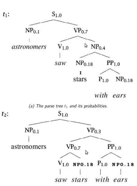
3.9 Two parse trees for the sentence astronomers saw stars with ears. . . 31
4.1 Block diagram for the general system descripted. . . 33
4.2 Block diagram for a regressor problem. . . 34
4.3 The block diagram with detail view of Song Semantic Model. 35 4.4 Valence-Arousal representation for two songs in the MsLite data set . . . 36
4.5 Semantic Equalizer representation for two songs in the MsLite data set . . . 39
4.6 System block diagram with detail view for Concept Modeling. 39 4.7 Concept modeling for words "hard" and "soft" on the hard-dimension. . . 42
4.8 Concept modeling for tempo markings words as listed in table 4.4. . . 43
4.9 System block diagram with detail view of computational core. 44 4.10 System block diagram with detail view of Query Modeling
module. . . 45
4.11 Flux diagram for songs retrieval in semantic example descrip-tion. . . 47
4.12 System block diagram with detail view for Scores Computing module. . . 53
4.13 The homepage for research. . . 56
4.14 Block diagram with detailed view of the visualization module. 56 4.15 An example of ranking list visualization. . . 57
4.16 An example of playlist visualization. . . 58
5.1 Skills owned by our survey population . . . 61
5.2 Music listening profiles in test population. . . 63
5.3 Histogram of evaluation rates for the query "I want a song very groovy and happy". . . 64
5.4 Histogram of evaluation rates for the query "I want a song not happy at all, dull and flowing". . . 65
5.5 Histogram of evaluation rates for the query "I want a playlist that sounds angry, fast and rough". . . 66
5.6 Histogram of evaluation rates for the query "I would like to listen to calm songs, like "Orinoco Flow", flowing and slow". . 67
5.7 Histogram of evaluation rates for the query "I want a playlist not angry, and not stuttering and with a slow tempo". . . 67
5.8 Histogram of evaluation rates for results of free-text queries. . 69
5.9 Histogram of evaluation rates for usefulness of the system. . . 69
5.10 Histogram of evaluation rates for the question about personal potential use of the system. . . 70
5.11 Histogram of evaluation rates about the general concept of the syste. . . 71
List of Tables
3.1 Low and mid-level features used in this work . . . 20
4.1 List of high-level semantic descriptors chosen from the anno-tation experiment in [2] . . . 37
4.2 List of NEDs in this work . . . 38
4.3 Notation used for song semantic models . . . 40
4.4 Tempo markings and correspondent ranges of BPM . . . 42
4.5 Notation used for concept models . . . 44
4.6 Verbal labels and correspondent mean values from [3] . . . 48
4.7 Notation used for query models . . . 52
4.8 Notation used for scores . . . 55
5.1 Rate neighborhood for false-positive outliers recover . . . 62
5.2 Linear Regressor and Robust Linear Regressor Root Mean-Square Errors for each non-emotional high-level descriptor. . . 62
5.3 Evaluation for the predefined queries . . . 64
5.4 Evaluation for the system’s general aspects. . . 68
Chapter 1
Introduction
Music has always had an important role in the human life. The advent of the digital era has considerably increased the amount of music content that users can accede to. Most part of the music published in the last century is on sale online. Thousands or even millions of songs can be stored in media storage. The amount of music currently available is more than a person can listen to in an entire life. This information overload leads to an evolution in music listening experience. Until today mediators, such as music dealers and music magazines, have played an important role in collecting, organizing, retrieving and suggesting music for people. Users can now directly access to music via Internet and mediators risk to disappear. The music organization reflects the taxonomy used by mediators to classify music and is based on meta information such as title, album name, artist, year and so on. Nevertheless, people have recently been using to reach and listen to music without knowing any information about it. Users habits are changing: on one side people keep listening to music by a certain artist or belonging to a certain genre; on the onther side, they listen to music that inspire a certain mood or that has a certain sound.
New applications and paradigms are needed to collect, suggest, organize and retrieve music for people. Scientific community and industries are work-ing to build automatic mediators that can address these issues. In order to realize this, it is crucial to investigate about music content, how to model it and which aspects are significant for representing it. On the other side, it is important to investigate how users understand music content, which descrip-tion they use for it and how they would like to access it. For example, one of the main prerogative of music is to inspire feelings to listeners. People use to choose their music according to the mood they are feeling or in order to be brought to a certain emotion. Nevertheless, other non-emotional factors
6 Chapter 1. Introduction
are taken into account when listening to music, such as musical genre (rock, pop), rhythmic aspects (slow, fast, dynamic) or other generic descriptors used in common language (dull, easy, catchy, noisy).
The gap between users and music content must be filled in order to build novel mediators. Music Information Retrieval (MIR) community studies and investigates elements involved in users description and music content. MIR is a multidisciplinary research field that deals with the retrieval and processing of information from music. MIR disciplines include: musicology, psychology, psychoacoustic, academic music study, signal processing, computer science and machine learning. Music information can be formalized and described hierarchically from lower level, which is related to sound content, to higher level, which is related to perception of sound. These information are re-ferred to as descriptors or features. Low-level features (LLF) are directly extracted and computed from the audio signal and describe information re-lated with Spectral or Energy components. They are extremely objective, but they poorly describe music to users. High-level features (HLF) carry a great significance for human listeners, hence they are the most feasible for wide-diffusion application. They are very subjective, since they give the higher level of abstraction from the audio signal they refer to. They can represent related descriptors of music (ED) or to non emotional-related (NED). Mid-level features (MLF) represent the middle layer between low- and high-level features. MLFs introduce a first level of semantics and combine LLFs with musical and musicological knowledge. In MIR literature, the gap between users description and music content is referrered to as gap between low-level and high-level features.
New paradigms need an accurate high-level music description. HLFs can be manually annotated by human listeners (context-based), but this ap-proach is impractical, due to the large amount of music availability and the high subjectivity of the annotation. HLFs can also be based on a set of LLFs (content-based), but this is a hard task that involves machine learning prediction techniques. In the current situation, context-based approaches are mainly used in applications that interact with users, hence via HLFs, whereas content-based approaches have usually been limited to applications dealing with the audio content, hence via LLFs. In chapter 2 we will give an overview of these applications. An application that interacts with users and addresses the issue of wide music availability should be content-based and describe music by means of HLFs.
The representation of HLFs has two approaches: cathegorical and dimen-sional. The cathegorical approach tends to assign binary value descriptors to music. That is, a song can be either descripted or not descripted by a
7
feature, such as rock or not rock. In the dimensional approach, it is possible to quantifies how much a feature describes a song, e.g., in a 9-point scale from 1 to 9, this song has a value of roughness equal to 7.
With particular respect to emotional-related descriptors, Music Emotion Recognition (MER) is a research field that aims at investigating how to conceptualize and model emotions perceived from music. Dimensional ap-proach to MER aims at representing emotions in a continuous (dimensional) space. The most referred space in the literature is the Valence and Arousal 2-dimensional space (AV). The Valence concerns how much a mood is positive or negative, whereas the Arousal is related to the energy of the emotion (ex-citing or calming). Sometimes an additional dimension, called Dominance, is considered. It represents the sense of control or freedom to act of an emotion [1] (AVD space). For the purposes of Music Emotion Recognition, songs are mapped as points in the AV or AVD space. The points represent the feelings inspired by the songs.
Technology is experiencing another kind of evolution, related with user interaction. Inputs to the computer changed from command-line terminal to windows environment and are moving to touch-screen interaction and gesture commands. Nowadays an user-friendly interface is a basic design requirement for any application. New systems seem to be oriented to the comprehension of users’ requests by allowing people to communicate as most intuitively as possible. Natural Language Processing (NLP) is a discipline that concerns making machines able to understand human natural language. Through NLP, users might communicate their requests to a machine as they were talking to a human. One of the most relevant NLP application1
is Siri2
, the Apple’s voice assistant. It is able to receive commands in natural spoken language and translate them into directives for the device operative system. Music search is one of the challenge that MIR community is facing. A first approach for music search involves with taking meta information (such as title or artist) from the user and returning the correspondent music content. This kind of music indexing does not consider any information about actual music content, neither at high level nor at low level. In the new music scenario, users may want to retrieve music without having any information about it, but only an idea on what to retrieve. In order to invert the process, some kind of description for music must be provided. Here are some examples of type of query for MIR applications:
1How innovative is Apple’s new voice assistant Siri,
http://www.newscientist.com/article/mg21228365.300-how-innovative-is-apples-new-voice-assistant-siri.html
8 Chapter 1. Introduction
• by humming: the user sings or hums the song;
• by tapping: the user taps the rhythm pattern of the song;
• by beatboxing: the user emulates the rhythm pattern of the song by beatboxing it;
• by example: songs are retrieved by similarity to one provided; • by semantic description: the user describes the song by text.
In this thesis we address the problem of song retrieval in a content-based manner by text-based natural language query. The purpose of this work is to create a music search system using query by semantic description. We aim at processing natural language query in order to exploit the richness of lan-guage and to capture the significant concepts of the query and qualifiers that specify the intensity desired. In this thesis we will use words and concepts as synonyms. We analyze emotional and non emotional-related description by means of semantic high and mid-level features. We use dimensional approach both for EDs (by the Valence-Arousal space) and NEDs. Song similarity can also be specified in the semantic description. The similarity among songs is intended as similarity among songs’ semantic descriptions. The system com-bine content-based approach for the annotation and high-level features for the descriptions, hence we propose a intuitive system for users and scalable for large amount of music. We named the system Janas, from an ancient Sardinian word that means fairies. With this word, we refer to the ancient era when music and magic were considered deeply bound.
We implemented a prototype of the system as a web search engine that outputs a ranked list of songs or a playlist. However, there are several possi-ble applications. Web digital-media store may use it in order to suggest songs from free text-based queries or by content similarity with previous orders. This system may be used as an automatic playlist generator for music player softwares or in portable music devices. Users may also be interested in the possibility of searching among their personal music collection via semantic queries.
This thesis is organized as follows. Chapter 2 presents an overview of the state of the art for: main music search engines systems, music recom-mendation systems, high-level descriptors used in commercial application or proposed by the MIR community, latest paradigms for music browsing. In Chapter 3 we list and explain tools and theoretical background we needed to develop our project. We cover: Bayesian decision theory, natural language sentence parsing, audio features, emotional-related HLFs, machine learning
9
regressors for generating content-based HLFs. In chapter 4 we discuss details of the implementation of system under discussion. In chapter 5 we describe experimental results and the data set we used to collect them. Chapter 6 analyzes conclusions and possible future applications for the system we present.
Chapter 2
State of the art
In this chapter we will provide an overview of the state of the art for Music Information Retrieval researches and applications. We will start with an overview of the high level features currently used to describe music. We will then describe the most relevant music recommendation systems currently available, from commercial and research fields. The third section concerns music representation and navigation, i.e. the solutions introduced to over-come the standard classification of songs (name, artist, genre). In the last section we will discuss the current efforts in Music Information Retrieval for the searching and retrieve of music.
2.1
High-level Features
High-level features describe music with a high level of abstraction. High-level features are usually divided in emotion-related and non emotion-related. The latter include descriptors for a wide variety of music characteristics.
In [4] the author introduces a set of bipolar-continuous NEDs for high-level perceptual qualities of textural sound modeling. The descriptors considered are: high - low, ordered - chaotic, smooth - coarse, tonal - noisy and homo-geneous - heterohomo-geneous. Such descriptors are suitable to describe textural sound, i.e., abstract and environmental sounds, but they are not for more complex sounds like songs.
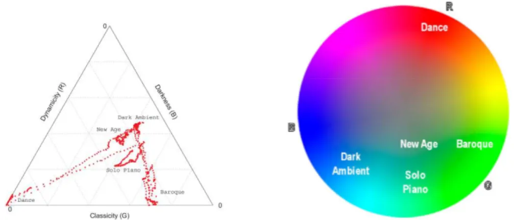
In [5] the authors train a SVM learning machine to classify music genres. They find three high-level features able to represent and visualize genres. Such features are: darkness, dinamicity and classicity. They use these fea-tures to map songs’ time-varying evolution among the genre space. Although these features seem to have a high descriptive potential, they do not have an intuitive definition for the generic user. A visualization of music genre is
12 Chapter 2. State of the art
shown in figure 2.1.
(a) Resulting triangular plot for mixed genre stream test.
(b) Resulting average genre colors for mixed genre stream test.
Figure 2.1: Visualization of high-level features obtained through the analysis of the heterogeneous music stream
In [6] the authors describe a system for semantic annotation and retrieval of audio content. The annotation and retrieval is based on a vocabulary, descripted in [7] of 159 cathegorical semantic descriptors1
, divided in: • emotion: concerns feelings inspired by the songs;
• genre: the musical genre of the songs;
• instrument: the instruments played during the song, included male and female lead vocals
• song: some general aspects such as changing energy level or catchy/memorable; • usage: typical situation for listening that particular song e.g., at a
party, going to sleep and so on);
• vocals: the style or features of the singer, such as duet or breathy. In [8] the authors present a system that hierarchically classify recordings by genre. They extract 109 musical features divided in seven main cathe-gories:
• Instrumentation (e.g. whether modern instruments are present);
1CAL-500 semantic vocabulary for music analysis,
2.2. Music recommendation systems 13
• Musical Texture (e.g. standard deviation of the average melodic leap of different lines);
• Rhythm (e.g. average time between attacks);
• Dynamics (e.g. average note to note change in loudness); • Pitch Statistics (e.g. fraction of notes in the bass register); • Melody (e.g. fraction of melodic intervals comprising a tritone); • Chords (e.g. prevalence of most common vertical interval).
These HLFs exhibit good performances in genre classification. Nevertheless they have been extracted from MIDI symbolic recordings, hence they have not been proofed in a real-world situation with actual audio signal.
2.2
Music recommendation systems
Music recommendation systems help users to navigate among the large amount of available music by suggesting songs that match their musical tastes. Context-based approach for music recommendation is limited to the comparison of users’ music libraries for songs suggestion. Content-based approach can also focus on song actual content for the retrieval of songs similarity.
Genius is an automatic playlist generator inside the software iTunes2
. Once it has created a playlist, it also suggests songs from the Apple Store that matches similarity with the songs in the user’s library. Although no formal description of the algorithm has been provided, it is probably based on context similarity among users’ libraries3
. Last.fm4
is a website founded in 2002, that builds a profile of user’s musical tastes from Internet radio stations or computer’s music player. Starting from this profiling, Last.fm provides a service of recommendations for new music, based on context-based similarity with other profiles.
In [9] the author provides a description of a music recommendation system based on context, content and user profiling. The context based information are gathered from music related RSS feeds. The content-based information is extracted from the audio. Finally, profiling information about user’s listening habits and user’s friends of friends’ interests are considered during the music recommendation process.
2Apple Inc., http://www.apple.com/itunes/
3"How iTunes Genius Really Works",
http://www.technologyreview.com/view/419198/how-itunes-genius-really-works/
14 Chapter 2. State of the art
All the content-based recommendation systems discussed above do not allow to drive the recommendation and they are mainly based on personal musical tastes. The system we propose in this work allows people to choose personal criteria for music recommendation.
2.3
Music browsing
Music has been traditionally listened to and browsed following classical tax-onomy. People used to listen to music by an artist, or from an album, or matching some favorite genre. This was not sufficient and people started to create playlist of different artists, albums or genres with the intent to col-lect and browse music that matched other aspects of music, such as relaxing songs while studying or positive and fast songs while jogging. Music browsing differs from music recommendation because the former aims at suggesting music similar to users’ tastes, whereas the latter provides ways to organize music. In this section we will present some applications that browse music and the features they use to organize it.
Pandora5
is a website that provides a customized web radio station similar to users’ tastes. It is based on the Music Genome Project6
, that aims to capture the essence of music at the fundamental level using a set of almost 400 attributes. Since the features are context-based and manually annotated, songs are limited to the ones just included in the Pandora database and not easily scalable.
Stereomood7
is a website for music streaming depending on the mood or emotions felt. Once the user has chosen that particular feeling, Stereo-mood generates a playlist of tracks that match that Stereo-mood. The database is composed by context-based annotations and it contains also annotations not directly related to objective but inspires mood, such as sunday morning or it’s raining.
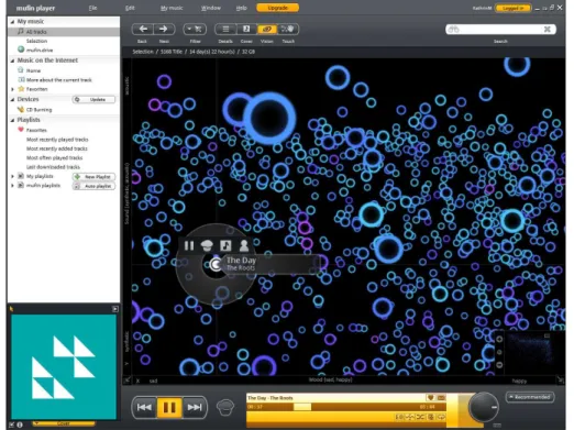
Mufin8
is a service that includes music player and cloud storage functional-ities. Users’ songs are uploaded and analyzed by Mufin, that maps them in a sort of Valence-Arousal space extended with a synthetic-acoustic dimension. Users can have a 3D view of their music into this space and create playlists by mood neighboring. The mapping follows a content-based approach, hence no manual annotation by the user is needed. A screenshot of its 3D view of songs is shown in figure 2.3.
5Pandora, http://www.pandora.com
6The Music Genome Project, http://www.pandora.com/about/mgp 7Stereomood srl., http://www.stereomood.com
2.3. Music browsing 15
Figure 2.2: The interface of Moodagent for Android devices.
Mood Agent9
is a music player that uses four high-level emotional-related descriptors (sensual, tender, happy and angry) and one mid-level feature (the tempo) to create a playlist based on music similarity. The analysis on music is content-based and the playlists are built tuning descriptors as they were sliders on an equalizer. Its interface is shown in 2.2.
Musicovery10
is a website and mobile ap-plication that maps songs in a quantized Valence-Arousal plane. Selecting an area in the VA plane, the user can play a song according to a certain mood. It also pro-vides a tool to play songs starting from an artist and finding similar songs. Its algo-rithm is based on a set of 40 acoustic fea-tures context-based (annotated by an expert at Musicovery11
) that are pro-cessesed to find the mood of the song.
In [10] the authors describe an approach to multimedia playlist genera-tor based on prior information about musical preferences of the user. The playlist generator can be driven by environmental or unintentional signals and by intentional control signals. The features selected as control signals are mood, brightness and RMS to specify loudness. It is also possible to tap the desired tempo. Features are content-based and refer to excerpts of song, in order to dynamically build the playlist (on fly). Since the system takes into account also the history of the system in order to capture the preferencies of the user, it can be seen as in-between music browsing and recommendation.
Most of these systems use only an emotional description to navigate among songs; those which do not, are based on just one typology of description. In this work, we combine together semantic emotional and non emotional-related description in order to provide a higher degree of freedom for user.
9Syntonetic, www.moodagent.com 10Musicovery, www.musicovery.com
16 Chapter 2. State of the art
Figure 2.3: The interface of Mufin Player.
2.4
Music search and retrieve
Music search engines offer the possibility to retrieve songs by describing its content. They do not aim at organizing music or recommending it. In the latest decades some applications were created to retrieve songs by an analysis of their actual content.
Soundhound12
is a mobile phone application that allows to search and re-trieve music via query by humming. Soundhound is the rename of Midomi13
, a website for music search via query by humming. In Midomi, researches are made among both original songs and recordings sent by users, using features as pitch, tempo variation, speech content and location of pauses14
. Shazam15
is a popular mobile application that accepts music excerpts recorded by the microphone of the mobile device and retrieve the song recorded. The algorithm faces several problems, such as low quality
record-12Soundhound Inc. http://www.soundhound.com 13Midomi, http://www.midomi.com
14"This Website can name that tune",
http://news.cnet.com/This-Web-site-can-name-that-tune/2100-1027_3-6153657.html
2.4. Music search and retrieve 17
ings or ambient noise. In [11] the author gives a description of the algorithm that extract a robust fingerprint by building a so-called costellation map from the spectogram of the recorded audio.
In [12] the author builds a semantic space for queries and an acoustic space for audio signals. The semantic space uses a hierarchical set of multinomial models to represent and cluster a collection of semantic documents. The acoustic space uses a signal processing chain composed by Mel-frequency Cepstral Coefficient (MFCC) extraction, stacked together through frames, analyzed by linear discriminant analysis (LDA) and finally feed to a Gaussian mixture model recognizer. The two spaces are linked together by another gaussian mixture model. This approach has good performance for the ex-periment proposed by the author, that relies on short audio fragments and simple semantic queries. It is tailored on analyzing the objective content of an audio signal (what is recorded) rather than qualities of a song (how it sounds).
In [6] the authors create a system of music information retrieval based on semantic description queries. To overcome the lack of data set semantically labeled, they collect a dataset of 500 songs from humans’ listenings and an-notations. The data set, named Computer Auditory Lab 500 (CAL500) is currently available online16
. The songs have been modeled as GMM distri-butions by an Expectation-Maximization algorithm (EM). Using the models found, they also realize an automatic semantic annotator for songs.
Queries by humming or by example are useful to retrieve a certain song, but they cannot (and are not intended to) be used for music recommendation. The semantic information retrieval systems discussed are more similar to our work. In addition, we exploit the richness of language using a natural language processing module in order to accept complex queries. Moreover, our mood vocabulary considers about 2000 emotions.
Chapter 3
Theoretical Background
In this chapter we will present the theoretical background needed for our work. In the first section we will introduce some Music Information Retrieval methods. We will first analyze the audio features and the regressors we used in building a content-based data set. We will also give an overview the Music Emotion Recognition field. In the second section we will provide the fundamentals of Bayes decision theory we based our work on. In the last section we will present Natural Language Processing definitions and we will focus on the problem of sentence parsing and the solution we chose.
3.1
Music Information Retrieval
Music Information Retrieval is a multidisciplinary research field that deals with music information. Music information is expressed by features or de-scriptors. Music features are classified according to their level of abstraction: low-level features are the most objective, whereas high-level features carry the greatest semantic significance.
3.1.1 Audio Features
Low-level features, also referred to as audio features, can be classified on the acoustic cues they are capturing. LLFs can measure: the energy in the audio signal, its distribution and its related features (such as loudness and volume); the temporal aspects related with tempo and rhythm; some attributes related with the spectrum. In the following, we will illustrate the features we employed in this work, as descripted in [13]. The list of the features is shown in table 3.1.
20 Chapter 3. Theoretical Background
Low-level
Spectral MFCC, Spectral Centroid, Spectral Flux,
Spectral Rolloff, Spectral Flatness, Spectral Contrast
Mid-level
Rhythmic Tempo
Table 3.1: Low and mid-level features used in this work
Mel-Frequency Cepstrum Coefficients
Mel-Frequency Cepstrum Coefficients (MFCCs) are spectral LLFs that are based on Mel-Frequency scale. Mel-Frequency scale models the human au-ditory system’s perception of frequencies. MFCCs are obtained from the co-effiecients of the discrete cosine transform (DCT) applied on a reduced Power Spectrum. The reduced Power Spectrum is computed from the log-energy of the spectrum pass-band filtered by a mel-filter bank. The mathematical formulation is:
ci =PKk=1c {log(Ek)cos[i(k −12) π
Kc]} with 1 ≤ i ≤ Nc, (3.1)
where ci is the i − th MFCC component, Ek is the spectral energy measured
in the critical band of the i − th mel-filter, Nc is the number of mel-filters
and Kc is the amount of cepstral coefficients ci extracted from each frame.
Spectral Centroid
Spectral Centroid is the center of gravity of the magnitude spectrum. Given a frame decomposition of the audio signal, Spectral Centroid is computed as: FSC= PK k=1f (k)Sl(k) PK k=1Sl(k) , (3.2)
where Sl(k) is the Magnitude Spectrum at the l − th frame and the k − th
frequency bin, f (k) is the frequency corresponding to k − th bin and K is the total number of frequency bins. Spectral Centroid can be used to check whether the magnitude spectrum is dominated by low or high frequency components. It is often associated with the brightness of the sound. Spectral Centroids for two songs are shown in figure 3.1.
3.1. Music Information Retrieval 21 60 65 70 75 80 85 90 1000 2000 3000 4000 5000 6000 7000 8000 Spectral centroid, 190.mp3
Temporal location of events (in s.)
coefficient value
(a) Disturbed - "Down with the Sickness"
60 65 70 75 80 85 90 0 1000 2000 3000 4000 5000 6000 Spectral centroid, 019.mp3
Temporal location of events (in s.)
coefficient value
(b) Henya - "Orinoco Flow" Figure 3.1: Spectral Centroid for two songs.
Spectral Flux
Spectral Flux captures the spectrum variations, computing the distance be-tween the amplitudes of the magnitude spectrum of two successive frames. We consider the Euclidean distance:
FSF = 1 K K X k=1 [log(|Sl(k)| + δ) − log(|Sl+1+ δ|)]2, (3.3)
where Sl(k) is the Magnitude Spectrum at the l − th frame and at the k − th
frequency bin and δ is a small parameter to avoid log(0). A representation of Spectral Flux for two songs is shown in figure 3.2.
60 65 70 75 80 85 90 0 100 200 300 400 500 600 700 Spectral flux, 190.mp3
Temporal location of events (in s.)
coefficient value
(a) Disturbed - "Down with the Sickness"
60 65 70 75 80 85 90 0 50 100 150 200 250 300 Spectral flux, 019.mp3
Temporal location of events (in s.)
coefficient value
(b) Henya - "Orinoco Flow" Figure 3.2: Spectral Flux for two songs
Spectral Rolloff
Spectral Rolloff represents the lowest frequency FSRat which the value of the
22 Chapter 3. Theoretical Background
amount of the total sum of the magnitude spectrum. Spectral Rolloff is formalized as: FSR= min{fKroll| Kroll X k=1 (Sl(k)) ≥ R K X k=1 (Sl(k))}, (3.4)
where Sl(k) is the Magnitude Spectrum at the l − th frame and the k − th
frequency bin, K is the total number of frequency bins, Krollis the frequency
bin index corresponding to the estimated rolloff frequency fKroll and R is
the frequency ratio. In [14] authors consider R at 85% whereas in [15] R is fixed at 95%. Spectral Rolloff is shown in figure 3.3.
60 65 70 75 80 85 90 3000 4000 5000 6000 7000 8000 9000 10000 11000 12000 Rolloff, 190.mp3
Temporal location of events (in s.)
coefficient value (in Hz.)
(a) Disturbed - "Down with the Sickness"
60 65 70 75 80 85 90 0 2000 4000 6000 8000 10000 12000 Rolloff, 019.mp3
Temporal location of events (in s.)
coefficient value (in Hz.)
(b) Henya - "Orinoco Flow" Figure 3.3: Spectral Rolloff for two songs with value R = 85%
Spectral Flatness
Spectral Flatness gives a measure of how much an audio signal is noisy, estimating the similarity between the magnitude spectrum of the signal frame and the flat shape inside a predefined frequency band. It is computed as:
FSF = KqQK−1 k=0 Sl(k) PK k=1Sl(k) , (3.5)
where Sl(k) is the Magnitude Spectrum at the l − th frame and the k − th
frequency bin, K is the total number of frequency bins. A representation for two songs is shown in figure 3.4.
Spectral Contrast
Spectral Contrast captures the relative distributions of the harmonic and non-harmonic components in the spectrum. They have been introduced in order to compensate the disadvantage of spectral information reducing. It is defined as spectral peak, spectral valley, and their dynamics separated into different frequency sub-bands.
3.1. Music Information Retrieval 23 60 65 70 75 80 85 90 0.05 0.1 0.15 0.2 0.25 0.3 0.35 0.4 Spectral flatness, 190.mp3
Temporal location of events (in s.)
coefficient value
(a) Disturbed - "Down with the Sickness"
60 65 70 75 80 85 90 0 0.05 0.1 0.15 0.2 0.25 Spectral flatness, 019.mp3
Temporal location of events (in s.)
coefficient value
(b) Henya - "Orinoco Flow" Figure 3.4: Spectral Flatness for two songs
Chroma features
Chroma features attempt to capture information about the musical notes present in the audio from its spectrum. The log-magnitude spectrum is mapped into a log-frequency scale, that corresponds to a linear scale for the music temperate scale. Given the frequencies of each note in a twelve-tone scale, regardless of the original octaves, a histogram of the notes is built. The result of such processing is called chromagram. Each bin represents one semitone in the chroma musical octave. A representation is shown in figure 3.5. 60 65 70 75 80 85 C C# D D# E F F# G G# A A# B Chromagram
time axis (in s.)
chroma class
(a) Disturbed - "Down with the Sickness"
60 65 70 75 80 85 C C# D D# E F F# G G# A A# B Chromagram
time axis (in s.)
chroma class
(b) Henya - "Orinoco Flow" Figure 3.5: Chromagram for two songs
Tempo
The tempo is a mid-level features that represents the speed of a given piece. Tempo is specified in beats per minute (BPM), i.e., how many beats must be played in a minute. Beat is defined as the temporal unit of a composition, as indicated by the (real or imaginary) up and down movements of a conductor’s hand[16].
24 Chapter 3. Theoretical Background
3.1.2 Regressor and machine learning algorithms
A learning machine is a system that deals with learning from data and pre-dicting new data. Given (xi, yi), i ∈ {1, ..., N } a set of N pairs, where xi is
a 1 × M feature vector and yi is the real value to predict, a regressor r(·) is
defined as the function that minimize the mean squared error (MSE) : ǫ = 1 N N X i=1 (r(xi) − yi)2. (3.6)
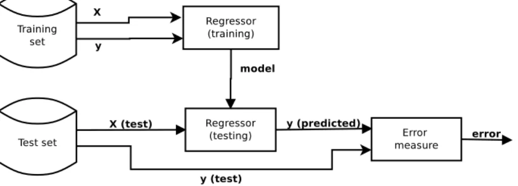
Features used for learning are called predictors. The set of pairs referred to as training set[17]. Given a training set, a regressor is estimated by two steps: the training phase and the test phase. In the training phase, the training set is used to estimate a regression function. In the test phase, a set of predictors with outcome available, called test set is used to estimate the performances of the regressor by comparison of the correct outcome and the output of the regressor. The block diagram of training and test phases is shown in figure 3.6.
Figure 3.6: Block diagram of training and test phases for a supervised regression prob-lem
In the following we will denote vectors with bold lowercase letters and matrices with bold uppercase letters.
Multiple Linear Regression
Linear regression starts from the assumption that there exists a linear rela-tionship between features and variables that must be predicted. Although this is a rare assumption, this kind of regression exhibits good performances. Multiple Linear Regression (MLR) is formalized as:
3.1. Music Information Retrieval 25
where X = [x1, ..., xN]T is the N × M matrix of features, β is the M × 1
vector of coefficients and ξ is the N × 1 vector of error terms. In order to minimize the MSE function between r(X) and y, where y is the expected output value, the least square estimator has the form:
β = (XTX)−1
XTy. (3.8)
The estimate value for a new 1 × M feature vector ˆx is estimated as:
r(ˆx) = ˆxβ. (3.9)
MLR is strictly dependent on the assumption that errors in the observed responses are normally distributed. A robust version has been developed to make MLR reliable in case errors are prone to outliers. The robust MLR method we used in our work is based on an iterative computation of weights of the regression function. Weights are assigned to each observation depend-ing on their distance from the prediction. Assigndepend-ing low weights to high distances leads to a lower regard to outliers.
3.1.3 Music Emotion Recognition
Music has always been connected to emotions. In fact, composers used to annotate mood markings on music sheets in addition to tempo indications (e.g., in a loving manner1
). This is a great help to provide the music play-ers additional information on the execution. The emotional description is one of the most intuitive for music. Indeed, as discussed in chapter 2, it is one of the most used in applications. Music Emotion Recognition (MER) is the field in MIR that studies the relationship between music and emo-tions. As mentioned before, two approaches are available for HLFs: the categorical and the dimensional. The former describes music with features that have a binary value, depending on whether a certain feature describes a song. The latter identifies how much a feature describes a song. In this study we focus only on dimensional approach. A dimensional approach for emotional-related descriptors involves the mapping of feelings and songs in a 2-dimensional plane, called Valence-Arousal (VA) plane. The Valence in-dicates how much the feeling is positive or negative, whereas the Arousal quantifies the energy of an emotion[1]. Mapping songs in the VA plane gives an immediate feedback about their emotional content. An approximated mapping of a few moods is shown in figure 3.7.
1amorevole. Music Dictionary, Virginia Tech,
26 Chapter 3. Theoretical Background
Figure 3.7: The 2D valence-arousal emotion plane, with some moods approximately mapped [1]
In [18] the authors mapped 2476 affective words in the Valence - Arousal - Dominance space. Most part of the semantic emotional-related description is based on their work.
3.2
Bayesian Decision Theory
A classifier is a learning machine that attempts to estimate from predictors a value in a discrete range of possible values [17]. Bayesian decision theory is a statistical approach for the problem of classification. It starts from the assumptions that the decision problem is posed in probabilistic terms and the probability values needed for classification are known. The Bayesian decision theory[19] explains how to use such probabilities to build a classifier.
3.2.1 Prior probability
Given an object s to be classified in one category si with i ∈ [1, N], the a
priori probability P (sj) is the probability that the object is sj. If no further
information was available, a logical decision rule for classification is:
3.2. Bayesian Decision Theory 27
Given a further information q depending on the state of s, the class con-ditional probability density function p(q|si) is the probability2 that q has a
certain value given an object known as si.
Given q and s, the posterior probability P (si|q) is the probability that s
is classified as si given the value q.
The joint probability density p(q, sj) is the probability that an object is sj
and has a certain value q, and it can be written as p(q, sj) = p(q|sj)P (sj) =
p(sj|q)P (q). Rearranging these leads to the Bayes formula:
P (sj|q) =
p(q|sj)P (sj)
P (q) (3.11)
where P (q) can be found as: P (q) =
N
X
k=1
p(sk)P (q|sk) (3.12)
Bayes formula states that posterior probability is computable as the prior probability times the class-conditional density function. The class-conditional density function p(q|sj) is the likelihood of sj with respect to q. The factor in
the denominator is a scale factor that ensures that all posterior probabilities sum to one. The Bayes decision rule for classification states:
classify s as sj if P (sj|q) = max(P (si|q)) with i ∈ [1, ..., N ]
(3.13)
3.2.2 Modeling the Likelihood function
Given a set of information q = [q1, q2, ...qm]T, we introduce a set of
dis-criminant functions gi(q) with i ∈ [1, N ] such that the classification rule
becomes:
classify s as sj if gj(q) = max(gi(q)). (3.14)
The discriminant function can be the posterior probability or some other measure dependent on the posterior probability such as:
gi(q) = p(q|si)P (si), (3.15)
gi(q) = ln(p(q|si)) + ln(P (si)). (3.16)
2We will use an uppercase P (·) to denote a probability mass function and a lowercase
28 Chapter 3. Theoretical Background
The conditional densities and prior probabilities are usually modeled as Gaussian densities or multivariate normal densities. A general multivariate normal density in d dimensions is written as:
p(x) = 1 (2π)d/2|Σ|1/2exp[− 1 2(x − µ) TΣ−1 (x − µ)], (3.17)
where x is a d-component column vector, µ is the d-component mean vector, Σis the d-by-d covariance matrix and |Σ| and Σ−1 its determinant and its inverse. We can model the conditional densities and prior probabilities as multivariate normal densities:
p(q) = 1 (2π)d/2|Σ|1/2exp[− 1 2(x − µq) TΣ−1 (x − µq)], (3.18) P (si) = 1 (2π)d/2|Σ i|1/2 exp[−1 2(x − µi) TΣ i−1(q − µ)]. (3.19)
With such modeling, the 3.16 becomes: gi(q) = − 1 2(x − µi) TΣ i−1(q − µ) − d 2ln(2π) − 1 2ln|Σi| + lnP (si). (3.20)
3.3
Natural Language Processing
The discipline of Natural Language Processing (NLP) deals with the design and implementation of computational machinery that communicates with hu-mans using natural language [20, Preface]. NLP includes a wide variety of researched tasks, such as automatic summarization, discourse analysis, nat-ural language generation, question answering. In this section we will fo-cus on parsing, i.e., determining the grammar analysis of a given sentence. We will first introduce the Part-of-Speech tagging and the Context Free Grammars[21]. We will then review the Probabilistic Context-Free Gram-mars and probabilistic sentence parsing [22].
3.3.1 Part-of-Speech tagging
Part-of-speech (POS) is a linguistic category of words, that is generally de-fined by its grammar role in a sentence. POS’s major categories are verbs and nouns. POS can be divided into two supercategories: closed class types and open class types. The former include those categories whose members’ amount can unlikely increase, like prepositions. The latter include categories like nouns or verbs, where new words often occur. Part-of-speech tagging is the process of assigning part-of-speech categories to word in a corpus. POS
3.3. Natural Language Processing 29
tagging faces several issues, like disambiguation (is book a noun or a verb?) and open class terms that may be unknown by the tagger. POS tagging can employ two main approaches: rule-based and stochastic. Rule-based ap-proach involve using disambiguation rules to infer the POS tag for a term. Stochastic approach computes probabilities:
P (word|tag) × P (tag|previous n tags) (3.21)
to classify a term with a certain tag. POS’s rules and probabilities are com-puted or inferred from previously annotated sentence corpus. POS tagging is useful in order to analyze the grammar of a sentence and its meaning. In order to represent a sentence, some kind of organization of POS is needed.
3.3.2 Context-Free Grammar
Figure 3.8: An example of parse tree representation of a Context-Free grammar derivation.
A group of words may behave as a single unit or phrase, called a constituent. For example, a noun phrase is a group of words linked to a single noun. A context-free grammar (CFG) consists of a set of rules, each of which expresses the ways that sym-bols of the language can be grouped and ordered together, and a lexicon of words and symbols. For example, a noun phrase (NP) can be defined as:
N P → Det N ominal. (3.22)
N ominal can be defined as:
N ominal → N oun|N oun N ominal, (3.23) i.e., a nominal can be one or more nouns. Det and N oun can be defined as well as:
Det → a; (3.24)
Det → the; (3.25)
N oun → f light. (3.26)
The symbols that are used in a CFG are called terminal if they corresponds to words (like the or f light) and non-terminal if they express clusters. We say that a terminal or non-terminal symbol is derived by a non-terminal symbol if it belongs to its group. A set of derivation in a CFG is commonly represented by a parse tree, where the root is called start symbol (see figure 3.8). A CFG is defined by four parameters:
30 Chapter 3. Theoretical Background
1. a set of non-terminal symbols N 2. a set of terminal symbols Σ
3. a set of productions P of the form A → α where A is nonterminal and α ∈ N ∪ Σ
4. a start symbol S
The CFG is suitable to parse a sentence, i.e., to represent a sentence as a parse tree that groups the constituents and explains the underlying grammar and words’ POS tags. A parse tree can be generated by means of a Probabilistic Context-Free Grammar.
3.3.3 Probabilistic Context-Free Grammar
A Probabilistic Context-Free Grammar (PCFG) is a probabilist model that builds a tree from a sentence using probabilities to choose among possible structures. It is formalized as a CFG where probabilities are considered in productions:
1. a set of non-terminal symbols N 2. a set of terminal symbols Σ
3. a set of productions P of the form A → β[p] where p is the probability that A will be expanded to β
4. a start symbol S
Such grammar can be used to parse sentences of language. Probabilities of expansions are inferred by means of machine learning techniques on previ-ously annotated sentences. PCFGs have been proofed to be a robust model, because implausible expansions have low probability. They also give a good probabilistic language model for English. In the example in figure 3.9 we show two probabilistic parse trees for the sentence astronomers saw stars with ears. The values on the nodes refer to the probabilities for that node to be derived from his father. We can see the starting point probability is equal to 1. We can compute the parse tree probabilities as:
P (t1) = 1.0 × 0.1 × 0.7 × 1.0 × 0.4 × 0.18 × 1.0 × 1.0 × 0.18
= 0.0009072
P (t2) = 1.0 × 0.1 × 0.3 × 0.7 × 1.0 × 0.18 × 1.0 × 1.0 × 0.18
= 0.0006804
(3.27)
3.3. Natural Language Processing 31
(a) The parse tree t1 and its probabilities.
(b) The parse tree t2 and its probabilities.
Chapter 4
Implementation of the system
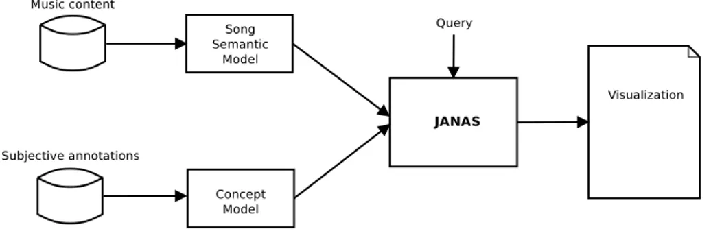
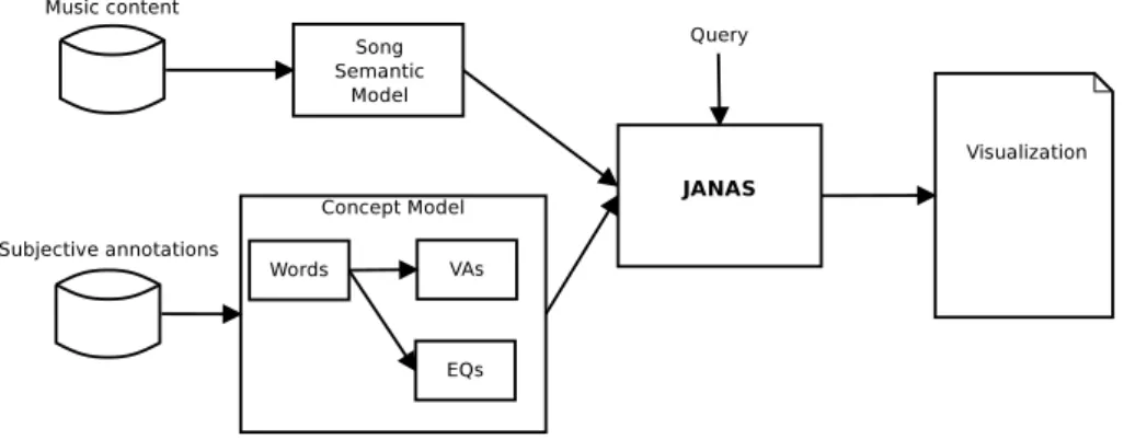
In this chapter we will describe the architecture of the system. The general scheme of the system is shown in figure 4.1. The system is composed by four main elements: i) a semantic model of songs; ii) a semantic model ofs concepts; iii) the computational core; iv) the visualization module.
Figure 4.1: Block diagram for the general system descripted.
For each song, two semantic models are derived by its music content. The first model refers to emotional-related description of the song, whereas the second refers to non emotional-related description.
A similar formalization is also used for concepts. A word is modeled either emotionally or non-emotionally, depending on its meaning.
Given the system is based on free-text query, the computational core parses the query to capture the key-words that are relevant for the research. The query can express: semantic emotional-related description; semantic non emotional-related description or song similarity. Semantic descriptions are mapped in the emotional- and non emotional-related concepts model. The song similarity is computed as similarity among songs’ semantic mod-els. This kind of research is defined query by semantic example (QBSE[23])
34 Chapter 4. Implementation of the system
since it considers similarity among semantic descriptions of the songs. The computational core uses the mapping to compute similarity scores that rep-resent how much a song match the query. In this chapter we will refer to the computational core as Janas.
The visualization module shows the results of computational core.
4.1
Music content semantic modeling
The system we propose deals with semantic text-based query based on emotional-and non emotional-related description. We used the data set proposed in [24], called MsLite. This data set is only annotated for ED, for this reason we ran a survey to annotate it for NEDs. From the survey we collected NED annotations only for a part of the data set. Because of this, we implemented an automatic annotation system in order to annotate the non-annotated songs. The NED conceptualization modeling system is based on regression functions explained in Chapter 3.
Figure 4.2: Block diagram for a regressor problem.
The general scheme for a regression procedure is shown in figure 4.2. For the purpose of regressors’ training, we built a training set. The training set was composed by LLFs extracted from the audio excerpts (as mentioned in chapter 3) as predictors and subjective annotations as outcome variables. We trained two regressors, a Linear Regressor and its Robust version. Since it exhibited the best performances in the training set, we use the Linear Regressor to predict non-emotional HLFs value for those excerpts that had
4.1. Music content semantic modeling 35
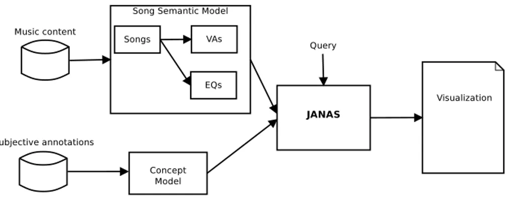
not been annotated. We modeled the non-emotional music content as nor-mal distributions, that are defined by the mean and the standard deviations. For annotated excerpts we used the means and the standard deviations of annotations, whereas for non annotated excerpts we used predicted values as means and root mean square errors as standard deviations. The root mean square errors for the two regressors are listed in table 5.2. The whole proce-dure of annotation and machine learning prediction is presented in chapter 5. The block diagram for the music content semantic modeling is depicted in figure 4.3. Each song is modeled, from its content, by a emotional-related model, we named VA, and by a non emotional-related model, we named EQ.
Figure 4.3: The block diagram with detail view of Song Semantic Model.
4.1.1 Emotional Descriptors
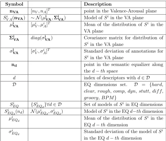
Emotions can be mapped in the 2-dimensional Valence-Arousal plane, whose axis are Valence (negative-positive) and Arousal (low-high energy). Songs are annotated in a 9-point scale from 1 to 9. For Valence, 1 is related to a very negative sensation and 9 to a very positive sensation, whereas for Arousal 1 is related to a sensation with no energy and 9 to an extremely energic sensation. The annotation provided in the MsLite depends on people musical tastes and personal perception. Given a set of Ki annotations from
testers {(v1,i, a1,i), ..., (vKi,i, aKi,i)} for a song S
i, where i = 1, ..., N is the
index of the song and N is the amount of songs in the data set, we obtained the mean µi
VA and standard deviations σVAi of annotation as:
µi VA = " µiV µiA # = " 1 Ki PKi k=1vk,i 1 Ki PKi k=1ak,i # , σVAi = " σi V σAi # = 2 q 1 Ki−1 PKi k=1(vk,i− µiV)2 2 q 1 Ki−1 PKi k=1(ak,i− µiA)2 . (4.1)
36 Chapter 4. Implementation of the system
We modeled the songs in the database as normal distributions in the Valence Arousal plane:
SV Ai (nVA) ∼ N (µiVA, ΣiVA), (4.2)
where N (·) denotes a normal distribution, ΣiVA= diag(σV Ai ) = " σVi 0 0 σi A # (4.3) is the covariance matrix and nVA = [nV, nA]T represents a point in the
Valence-Arousal plane. The emotional-related semantic distribution of the song is normalized as:
Z 9
1
Z 9
1
SV Ai (nV, nA)dv da = 1, (4.4)
in order the songs have the same probability. In figure 4.4 we show a repre-sentation of two songs modeled as the normal distribution. In the following we will refer to the emotional-related semantic model of a song as the song’s VA.
(a) Valence-Arousal representation for "Down with the sickness" by Disturbed.
(b) Valence-Arousal representation for "Orinoco Flow" by Henya.
Figure 4.4: Valence-Arousal representation for two songs in the MsLite data set
4.1.2 Non-Emotional Descriptors
Emotional features cannot describe music exhaustively. Indeed, non emotional-related features define a wide range of music qualities and, together with ED, may provide a more complete description. In [2] the authors proposed 27 se-mantic descriptors divided in affective/emotive, structural, kinaesthetic and judgement. For our study we have chosen to model a subset of their entire set of concepts. Specifically, we chose to model all the structural and one
4.1. Music content semantic modeling 37
judgement bipolar descriptors and one kinaesthetic descriptor, as shown in table 4.1.
In [2] the authors define the gesture descriptor as:
some aspect that makes a person start to move spontaneously. A similar definition is in [25], referred to the term grooviness:
a groove starts up and people stop whatever they are doing and begin to pay attention to the music; they either put their bodies in motion or adapt ongoing motion to follow the pull of the groove In [25], the author discusses the concept of grooviness. He attempts to find a clear definition for this descriptor, whereas in musicologist literature as among musicians no formal definition is provided1
. The capability of making people move is an important factor while choosing music, hence we considered grooviness descriptor in our NEDs’ set in substitution of gesture.
Semantic Descriptors Structural Kinaesthetic Soft/hard Gesture Clear/dull Rough/harmonious Judgement Void/compact Easy/Difficult Flowing/stuttering Dynamic/static
Table 4.1: List of high-level semantic descriptors chosen from the annotation experiment in [2]
The tempo indicates the speed of a song and it can affect general definition of a music piece. We have chosen to insert the tempo descriptors in the NEDs’ set. We indicated the tempo in beats-per-minute (BPM). For the tempo evaluation we used a VAMP plugin for the Sonic Annotator2
that is based on [26]. In [26] the authors define a beat tracker using a two state model. The first state performs tempo induction and tracks tempo changes, while the second maintains contextual continuity within a single tempo hypothesis. This is similar to the human tapping process. We manually corrected wrong-estimated tempi. Since we model songs as normal distributions, we needed
1The usual definition seems to be You know it when you hear it
38 Chapter 4. Implementation of the system
standard deviations. We computed standard deviation of a song’s tempo as an amount of tempo:
σiEQBP M = 0.125µiEQBP M, (4.5)
where µi
EQBP M is the computed tempo for the song S
i and σi
EQBP M is the
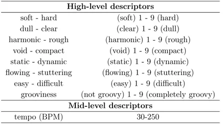
computed standard deviation. We have experimentally chosen 0.125 as the amount of tempo. The complete list of descriptors and their range of values can be found in table 4.2.
High-level descriptors
soft - hard (soft) 1 - 9 (hard)
dull - clear (clear) 1 - 9 (dull)
harmonic - rough (harmonic) 1 - 9 (rough)
void - compact (void) 1 - 9 (compact)
static - dynamic (static) 1 - 9 (dynamic) flowing - stuttering (flowing) 1 - 9 (stuttering)
easy - difficult (easy) 1 - 9 (difficult)
grooviness (not groovy) 1 - 9 (completely groovy) Mid-level descriptors
tempo (BPM) 30-250
Table 4.2: List of NEDs in this work
We computed means and standard deviations for the NEDs and we mod-eled the songs in the data set as normal distributions in 1-dimensional spaces, similarly to the adopted song model in the Valence-Arousal plane:
SEQi d(nd) ∼ N (µiEQd, σ
i
EQd) (4.6)
Where nd is a point in the mono dimensional space, d ∈ D is the index of
the descriptor and D = {hard, clear, rough, comp, dyn, stutt, dif f, groovy, BP M } is the set of NEDs. We represented the NEDs as nine juxtaposed bars, one for each descriptor. We called this representation semantic equal-izer. Each descriptor represents a slider that semantically equalizes the song (see figure 4.5). We define the whole non emotional-related semantic model for the song Si as the set:
SEQi = {SEQi d(nd)} with d ∈ D. (4.7)
In figure 4.5 we show a representation of two songs modeled in the normal distribution. In the following we will refer to the non emotional-related model of a song as the song’s EQ.
4.2. Concept modeling 39
(a) Semantic Equalizer representation for "Down with the sickness" by Disturbed.
(b) Semantic Equalizer representation for "Orinoco Flow" by Henya.
Figure 4.5: Semantic Equalizer representation for two songs in the MsLite data set
In table 4.3 we review the notation for the music content semantic models. Notice that given a song Si, Si
V A(nVA) is the model for the song’s VA,
whereas Si
EQ is a set of models for each dimension in song’s EQ.
4.2
Concept modeling
We modeled the songs in a semantic space. In order to retrieve them by means of semantic emotional- and non emotional-related descriptors, con-cepts need to be modeled in a similar semantic space. The block diagram for concept model is shown in figure 4.6. As we can see, the scheme for concept modeling is the dual of song modeling in 4.3.
![Figure 3.7: The 2D valence-arousal emotion plane, with some moods approximately mapped [1]](https://thumb-eu.123doks.com/thumbv2/123dokorg/7499661.104394/44.892.275.614.194.536/figure-valence-arousal-emotion-plane-moods-approximately-mapped.webp)