Issues in modelling and identification of Discrete Event Systems

(1)





        











































 





























(2)

Chapter 1 Preface

The term Discrete Event System (DES) was introduced in the early 1980s to identify an increasingly important class of dynamic systems in terms of their most critical feature: the fact that their behavior is governed by discrete events occurring asynchronously over time and solely responsible for generating state transitions. Examples of such behavior abound in technological environments such as computer and communication networks, automated man-ufacturing systems, air traffic control systems, C3_{I (Command,}

Control, Communication, and Information) systems, advanced mon-itoring and control systems in automobiles or large buildings, intel-ligent transportation systems, distributed software systems, mate-rial handling systems and so forth. The operation of such environ-ments is largely regulated by human-made rules for initiating or terminating activities and scheduling the use of resources through controlled events, such as hitting a keyboard key, turning a piece of equipment “on”, or sending a message packet. In addition, there are numerous uncontrolled randomly occurring events, such as a spontaneous equipment failure or a packet loss, which may or may not be observable through sensors.

DESs are particulary used in the field of the manufactured systems, handling systems and transportation systems: even if such system are being studying for long time, because of their complexity, they still present many issues that attract research

(8)

interest.

In particular this dissertation focuses about handling system modeling and DES identification.

Obtaining a good model of a system (both time-driven and event-driven) allows to more easily execute operations as perfor-mance analysis, control, monitoring of system evolution. However, in some cases modeling of a system is not simple because of several complications due to the behavior of the system or of the context it belongs to.

As example, sometimes, especially in the context of material handling and transportation, systems present both an event-driven and a time-driven behavior. In all that cases a very hight accuracy is not requested it is usual neglect the latter and “looking” at the system as a DES (as example modeling a handling system it is possible to be interested in knowing if a vehicle is or not in a zone of the path while it is not important to know its exactly position). When the time-driven behavior plays a fundamental role in the obtaining the overall system performance, such dynamics can not be neglected and they have to be explicitly modeled. This is the case, as example, of the automated warehouse systems, where the handling subsystem, as will be shown in the rest of this disser-tation, presents time-driven dynamics that greatly influence the warehouse’s performance. Consequently a new way to model the system behavior has to be used.

However, there are situation in which the difficult issue is not choosing the right formalism to model the system but it is the modeling itself.

This is typical in many practical contexts, where it can occur that one has to work with unknown ready made systems and no documentation about their behavior is available, or the model of a very complex system is needed. In these and other cases modeling becomes hard and another way to obtain the model of the system is needed: automated identification can be the solution.

(9)

1.1. Thesis contribution 3

1.1 Thesis contribution

In the modeling environment, contribution of this thesis consists in presenting a new methodology to obtain a model oriented to the control and performance analysis of complex material handling systems that is highly modular, compact and made of parameter-ized modules.

First a discrete event model is presented and then a new for-malism that merges the concepts of Hybrid Petri Nets and Colored Petri Nets is introduced: the Colored Modified Hybrid Petri Nets (CMHPNs). Hence a new CMHPN model is proposed: it allows to model both the event nature and the continuous nature of the system. As more, to allow the monitoring of system evolutions, a freeware simulation tool for the CMHPNs is presented.

Finally it is shown how the CMHPN model can be used to execute analysis and performance evaluation. Liveness analysis is performed by means of a hybrid automaton obtained from the net model. A deadlock prevention policy is synthesized working on an aggregated model. To prove the effectiveness of this new formalism an existing large automated warehouse system is presented as case study: its CMHPNs model is used to simulate the system behavior and to analyze the warehouse’s performance.

In the identification environments, the guidelines of a new “ac-tive” approach to identify the model of a preexisting system is described. The proposed preliminary algorithm identifies a free labeled PN model on the basis of the observed output sequences and of the modifiable input consisting of the enabled controllable transitions set.

The main idea is to use the knowledge of the set of enabled controllable transitions together with additional information on the conflicting transitions to accelerate the net identification with respect to the passive identification approaches. In particular, the system assumes that the maximum time that must elapse from the enabling of a transition until it fires is known and that it is possible to detect if the system is entered in a cyclic behavior. Using this additional information, it is possible to determine a

(10)

set of constraints to represent sequences that are not accepted by the system. Such constraints can be used to improve the net identification.

1.2 Thesis Overview

The thesis is organized as follow:

Chapter 2 contains a brief background on Petri Net (PN), Col-ored PN and Hybrid PN formalisms, necessary to un-derstand the others chapters. Because of their impor-tance in the developing of the contribute of this thesis, a brief literature review about the Hybrid PNs is also presented.

Chapter 3 introduces the problem of properly modeling a com-plex automated warehouse system and compares the proposed approach with the related works.

Chapter 4 describes two modular, compact, scalar approaches to model complex automated warehouse systems, the first based on the Colored Timed PN formalism and the second based on a new Petri net formalism that merges the concepts of Hybrid Petri Nets and Colored Petri Nets.

Chapter 5 presents a CMHPNs simulator that allows to design and simulate not only the net, but also the controller, allowing the user to create models ad hoc for several kinds of systems.

Chapter 6 deals with results obtained simulating the behavior of a real warehouse system.

Chapter 7 introduces the problem of the system identification. After a review of the existent literature, the guidelines of a new active algorithm are described.

(11)

1.2. Thesis Overview 5

Chapter 8 contains a summary table of the notations used in the dissertation.

(12)

(13)

Chapter 2 Notations and Definitions

In this Chapter the formalisms used in this dissertation are briefly recalled.

At first PNs are introduced. Then, a brief overview on CPNs is furnished. For further details on PNs and on simulation of Petri Nets (PNs), the reader can refer to [Mur89] and to [BCC07b].

Finally a background on the Hybrid Petri Nets (HPNs) is pre-sented.

2.1 Petri Nets (PNs) and Colored Petri

Nets (CPNs)

A Place/Transition (P/T ) net is a 4-tuple N =_{!P, T, Pre, Post",} where P is a set of w places (represented by circles), T is a set of n transitions (represented by black bars), Pre : P _{× T $→ N (Post :}

P_{×T $→ N) is the pre (post-) incidence matrix. C = Post−Pre}

is the incidence matrix. The net marking is represented as a vector m_{∈ N}m_{. The marking of a place p is a scalar value m}

p ∈ N. A

transition t is enabled at m iff m_{≥ Pre(·, t) and this is denoted as} m[t". An enabled transition t may fire yielding the marking m! ₌

m + C(_{·, t) and this is denoted as m[t"m}!_{. The symbols} •_{p (}•_t)

and p• _(t•_{) are used for the pre-set and post-set of a place p} _{∈ P}

(14)

As shown in Fig. 2.1(a), there is a structural conflict when

•_t

i∩•tj )= ∅. If ti and tj are both enabled, the conflict becomes a

behavioral conflict.

Let S =_{!N, m}0" be a Petri net system, where N is a PN and

m0 is its initial marking. Marking of S can be (partially)

observ-able. In such a case, it can be divided in m = [mO, muO], where

mO(muO) is the marking of observable (unobservable) places. We

call PO(PuO) the set of observable (unobservable) places.

A firing sequence from m is a sequence of transitions σ = t1. . . tk

such that m#t1"m1

#

t2"m2. . .

#

tk"mk, and this is denoted as m[σ"mk.

An enabled sequence σ is denoted as m#σ", while ti ∈ σ denotes

that the transition ti belongs to the sequence σ. The function

σ : T _{→ N, where σ(t) represents the number of occurrences of}

t in σ, is called firing count vector of the firing sequence σ. As it has been done for the marking of a net, the firing count vector is often denoted as a vector σ _{∈ N}n_{. Note that, if a sequence is}

made by a single transition, i.e., σ = ti, then the corresponding

firing count vector is the i-th canonical basis vector denoted as ei.

A marking m! _{is said to be reachable from m}

0 iff there exists

a sequence σ such that m0[σ"m!. R(N, m0) denotes the set of

reachable markings of the net system !N, m0".

A net system S is bounded if there exists a positive constant

K such that m(p)≤ K, ∀ m(p) ∈ R(N, m0).

A net system S is live if all its transitions are live. A transition

t is live under the initial marking m0 if for every marking m

reachable from m0, it exists a sequence σ, fireable from m, which

contains transition t. In other words, whatever the net evolution, a possibility always remains for firing t.

A PN system S = !N, m0" is said to be reversible if, for each

marking m _{∈ R(N, m}0), m0 is reachable from m. Thus, in a

reversible net one can always get back to the initial marking. The reachability graph of a bounded net S = _{!N, m}0" is a

directed graph RG such that: i) the root node of RG is the initial marking of the net; ii) the other nodes of RG are associated to the reachable markings of S; iii) an arc labeled t between two nodes X and Y of RG represents that the firing of transition t leads the

(15)

2.1. Petri Nets (PNs) and Colored Petri Nets (CPNs) 9

net system from the marking associated to the X to the marking associated to Y

A net system S =_{!N, m}0" is bounded, live and reversible iff its

reachability graph is finite, strongly connected and each transition t labels at least one arc [DHP+_93].

All the formal definitions given for PNs can be naturally ex-tended to Colored PNs (CPNs). Formally, a CPN is a 6-tuple C = _{!P, T, Pre, Post, Cl, Co". As in PNs, P is a set of m places} (represented by circles), T is a set of n transitions (represented

by bars). Cl is the set of colors. Co: P ∪ T −→ Cl is a

color function that associates to each element in P _{∪ T a}

non-empty ordered set of colors in the set of possible colors Cl. Forall p ∈ P, Co(pi) = {ai,1, ai,2, ..., ai,ui} ⊆ Cl is the ordered set of possible colors of tokens in pi, and ui is their number. Forall

t∈ T, Co(tj) =

!

bj,1, bj,2, ..., bj,vj "

⊆ Cl is the ordered set of possi-ble occurrence colors in tj, and vj is their number. For each place

pi ∈ P , the marking mi is defined as a non-negative multi-set

over Co(Pi). The mapping mi : Co(Pi) → N associates to each

possible token color in Pi a non-negative integer representing the

number of tokens of that color that is contained in the place pi.

The column vector of ui non-negative integers, whose h-th

com-ponent mpi(h) is equal to the number of tokens of color ai,h that are contained in pi, is denoted as mpi. The marking of a CPN is an m-dimensional column vector of multisets: m = [mp1...mpm]

T

. For the sake of simplicity, a token of color “c1” contained in a place pi will be indicated with the symbol (c1).

In literature, more than one formal definition for CPNs ex-ist, depending on how the incidence matrix and transition col-ors are defined. In the formalism chosen in this work, matrix entries are represented by matrices. Pre and Post are the pre-incidence and post-pre-incidence w_{× n-sized matrices, respectively.} Pre(pi, tj) is a mapping from the set of occurrence colors of tj

to a non-negative multiset over the set of colors of pi, namely,

Pre(pi, tj) : Co(tj)→ N(Co(pi)), for i = 1, ..., w and j = 1, ..., n.

Pre(pi, tj) represents a matrix of ui × vj non-negative integers

(16)

p t ₁ t ₂ (a) p t ₁ t ₂ (b)

Figure 2.1 Conflict in Petri Nets: (a) structural conflict and (b) behavioral conflict. 1 0 0 1 1 0 p t 1 t 2 ( c ₁_,1 ) ( c ₂_,1, c ₂_,2 ) ( c ₁, c ₂ ) (a) 1 0 0 1 1 0 p t ₁ t ₂ ( c ₁_,1 ) ( c ₂_,1, c ₂_,2) ( c 2 ) ( c 1 , c 2 ) (b)

Figure 2.2 (a) Unmarked CPN ; (b) Marked CPN.

the arc from place pi w.r.t color ai,h to transition tj w.r.t color

bj,k. Post(pi, tj) : Co(tj) → N(Co(pi)), for i = 1, ..., m and

j = 1, ..., n. Post(pi, tj) represents a matrix of ui × vj

non-negative integers whose generic element P ost(pi, tj)(h, k) is equal

to the weight of the arc from transition tj w.r.t color bj,k to place

pi w.r.t color ai,h. The incidence matrix C is a m× n matrix,

whose generic element C(pi, tj) : Co(tj) → Z(Co(pi)), for i =

1, ..., w and j = 1, ..., n, is the ui × vj matrix of integer

num-bers C(pi, tj) = Post(pi, tj)− Pre(pi, tj). The concepts of pre-set

and post-set of a place p _{∈ P or a transition t ∈ T are}

nat-urally inherited from PNs, but colors must be also considered:

•_t icj = ! ticj ∈ T | Pre(phck, ticj))= 0 " .

In Fig. 2.2(a) a CPN with a structural conflict is shown. it is made up of a place p, having Co(p) = {c1, c2}, and of two

transitions, t1 and t2 with Co(t1) = c1,1 and Co(t2) = {c2,1, c2,2}.

When t1 fires, one token, corresponding to color c1,1, is removed

from place p; t2 can fire both under color c2,1 and c2,2 and when

it fires, one c2,1 or c2,2 token, respectively, is removed from p. In

Fig. 2.2(b) a token is added to the CPN in Fig. 2.2(a); notice that the conflict is still structural (not behavioral), since no c1,1 token

(17)

2.2. Hybrid Petri Nets (HPNs) 11

is present in p and, consequently, transition t1 cannot fire.

When time is added to PNs and CPNs a time function is de-fined, which associates to each transition ti in the case of PNs, or

to each transition color ticj in the case of CPNs, a time duration

from enabling to firing. In this case the PNs and CPNs become TPNs and CTPNs. Notice that timed and un-timed (also said immediate in the next) transitions will be represented with empty filled boxes and black bars, respectively.

2.2 Hybrid Petri Nets (HPNs)

A hybrid system is defined like a system consisting of a mixture of a continuous time system and a discrete event system (DES), having each one an own state space. These two systems are not independent but they influence each other. For the continuous time system, the influence of DES results in abrupt changes in the dynamic and can occur either as switches in the vector field or as jumps in the state. Reversely, the continuous evolution influences the DES one by generating events that affect the discrete states [PL95].

A continuous system can be described by differential equations

˙x = f (x(t), u(t), t), x(0) = x0 (2.1)

y(t) = g(x(t), u(t), t) (2.2)

where x_{∈ R}n _{is the state vector, u}_{∈ R}m _{is the input vector and}

y∈ Rr_{is the output vector. In particular, if the interest is focused}

on the class of hybrid systems having autonomous commutations, i.e. systems for which changes in the dynamic occur if an analytical boundary condition about the instantaneous state value is reached, the equation ˙x = f (x(t), u(t)) (2.3) with f = $ f₁(x(t), u(t)) f or h(x(t)) _{≤ 0} f₂(x(t), u(t)) f or h(x(t)) > 0 (2.4)

(18)

can be used, where it has been supposed the system can switch

only between two possible dynamics (f1 and f2) and h is the

boundary condition.

For systems having linear, time-invariant, continuous part, like the ones treated in this thesis, each dynamic in (2.4) can be written as:

f_i(x(t), u(t)) = Ai· x(t) + Bi· u(t) (2.5)

where Ai is a constant n-order square matrix and Bi is a (n

×m)-order matrix.

To model hybrid systems behavior HPNs can be used [PL95, GU98, DA05, DPP09].

In more general hybrid systems, switching between different dynamics is caused not only by the boundary conditions but also by external input events, also called exogenous events. An ex-ogenous event, as the term suggests, is an event originating from the outside world; by opposition, a change in internal state, as the occurrence of a boundary condition, can be called endogenous event or internal event. The external events can be “controllable” (i.e. their occurrence can be forced/disabled by an external agent, for example by a controller) or not controllable (i.e. their occur-rence cannot be forced/disable by an external agent); an endoge-nous event is always not controllable. When changes in dynamic are ruled also by exogenous events, the HPNs used to model the system behavior are said synchronized, as those used in this dis-sertation: for these HPNs, an external event is associated with some transitions and the firing of these transitions occurs when the transition is enabled and the associated event occurs. Tran-sitions whose firing is controlled by the occurrence of an external or internal event are called “synchronized”. If the external event is a controllable event, then also transitions synchronized to such an event are called controllable, otherwise if a transition is syn-chronized to an uncontrollable event, then such a transition is said uncontrollable.

A HPN can be view as the combination of a “discrete” PN and a “continuous” PN.

(19)

2.2. Hybrid Petri Nets (HPNs) 13         Figure 2.3 A basic HPN.

is given in [DA05]; in [PL95] it is shown how HPNs can be used to describe a general hybrid system having jumps in the state space and switches in its dynamic. Application of HPNs to oil refinery can be found in [WZC08, WCZ09, WCCZ10].

Several variants of HPNs have been proposed. Differential Petri Nets (DPNs) are introduced the first time in [DK98]; in these nets the marking of a differential place may be negative as well as the weights of arcs to or from a differential place. In [DA05], it has been shown how the behavior of DPNs can be obtained us-ing HPNs whose transitions firus-ing speeds is a function of the net marking, and for this reason they are called Modified HPNs (MH-PNs) [DA05]. Then, it is not a limitation the use of no-negative markings and weights, as it is done in this dissertation.

To model systems having first-order continuous behavior, which can be studied by linear algebraic tools, Balduzzi et al. introduce the First-Order HPNs (FOHPNs) [BGM00] and use them to model manufacturing systems [BGS01]. In FOHPNs continuous transi-tion firing speeds are constant values, chosen by a control agent in a fixed range. When an event occurs, the net state changes, and a controller can decide to vary speed values, while between two event occurrences the firing speeds remain constant. In this thesis firing speed values are not chosen in a fixed set but they are function of the marking of the net.

In formal way, a HPN is a 7-tuple H =!P, T, Pre, Post, h, δ, ν" such that: P = PD%_PC_{, with P}D&_PC ₌ _{∅, where P}D _(PC₎

is the set of wd discrete ( wc continuous) places, drawn like one

(two) line circles; T = TD%_TC_{, with T}D&_TC ₌ _{∅, where T}D

is the set of nd discrete transitions, which can be both immediate

(drawn like black bars) and timed (drawn like white bars) and TC

(20)

Pre : P_{×T → R}+_{is the pre-incidence matrix; Post : P}_{×T → R}+

is the post-incidence matrix; h : P %T → {D, C}, called

”hy-brid function”, indicates for every node whether it is a discrete node (sets PD _{and T}D_{) or a continuous one (sets P}C _{and T}C_);

δ : TD _{→ (R}+₎nd _{is the firing delay vector, whose element δ}

i is

the firing delay associated to each discrete transition tD

i : if δi = 0

then the transition tD

i is immediate, else if δi > 0 then tDi is timed.

Function ν : Tc _{→ (R}+₎nc _{is the firing speed vector. Note that in} case of discrete nodes, Pre and Post assume integer positive val-ues. The incidence matrix of the net is defined as C = Post_−Pre and it can be written as the block matrix:

C = ' CCC CCD CDC CDD ( (2.6) where CCC is the block regarding connections between continuous

nodes, CDD is the block regarding connections between discrete

nodes, CCD is the block regarding connections between continuous

places and discrete transitions and CDC is the block regarding

connections between discrete places and continuous transitions. HPN marking is a function m = !mC_{, m}D"_{, with m}C _{: P}C _→

R+_{, m}D _{: P}D _{→ N, that assigns to each continuous place a real}

number and to each discrete place a nonnegative integer number of tokens (graphically represented as black dots in the discrete places). The notation m(τk) is used to denote the value of the

marking of the net at the instant τk. The marking of a place p at

a time τk is denoted by mp(τk). The symbols •p (•t) and p• (t•)

are used for the preset and postset of a place p _{∈ P (transition} t_{∈ T ), respectively, e.g.} •_{t =}!_p_{∈ P |Pre(p, t) > 0}"_.

A discrete transition tD _{is enabled at time τ}

k if mp(τk) ≥

Pre(p, tD_), _{∀p ∈} •_tD_{. A transition t}D _{can be either autonomous}

or synchronized to a logical expression, function of an external control input g and/or of an internal condition e. Both g and e

are boolean functions g, e : TD _{→ {0, 1}. The former becomes}

true, so generating an exogenous event, when a controller sets to true the external event it is associated to; the latter becomes true, so generating an endogenous event, when the internal event

(21)

2.2. Hybrid Petri Nets (HPNs) 15

it is associated to is verified. A discrete transition tD _{can fire if}

it is enabled and the associated logical expression becomes true, i.e. both the endogenous and the exogenous events its firing is synchronized to occur. As for example, in a system formed by two masses traveling along a guidepath, an internal condition can be associated to the reaching of a threshold distance that makes masses decelerate; an external control input for the same system is an asynchronous stop command arriving from an external con-troller; a logical expression can be the logic function AND between g and e, e.g. g_{∧ e.}

A continuous transition tC _{∈ T}C _{is enabled at time τ} k if i)

mD

pD(τk)≥ Pre(pD, tC), ∀pD ∈ •tCand ii) mC_pC(τk)≥ 0 ∀pC ∈ •tC.

To each continuous transition tC

i is associated the instantaneous

firing speed (in the following also called simply firing speed) νi:

if tC

i is disabled νi = 0; when tCi is enabled νi is equal to the

maximal firing speed ¯νi, indicated near the transition. The

fir-ing of continuous transitions cannot change the markfir-ing of dis-crete places, consequently CDC(pD, tC) = 0, ∀pD ∈ PD, thus

CDC = 0. The time derivative of the marking of a continuous

place pC_, dmpC

dt , is called balance and it is defined as: ˙mpC = I−O

where I =)_tC

j∈•pCP ost(p

C_{, t}C

j)νj is the feeding speed of the place

pC_{, while O =})

tC

k∈pC •P re(p

C_{, t}C

k)νkis the pC draining speed. The

evolution of the net can be described by its fundamental equation (written in a way pointing out the continuous part and the discrete part): ! mC_(τ k) mD_(τ k) " = ! mC_(τ k−1) mD_(τ k−1) " + + ! CCC CCD 0 CDD " # ! 0 σ(τk)− σ(τk−1) " +$τk τk−1 ! ν 0 " % (2.7)

where σ(τk) : TD → Nnd is the discrete firing vector whose

com-ponent σ_tD

i (τk) represents the number of times the discrete tran-sition tD

i is fired up to the current time τk.

For the sake of clarity, from now on the term “synchronized transition” will not be used any more and synchronized transitions

(22)

will be called just controllable or uncontrollable. A basic HPN is shown in Fig. 2.3, having: • PC ₌!_p 1 " , PD ₌!_p 2, p3 " ; • TC ₌ !_t 1 " , TD ₌ !_t 2, t3 "

where t3 is an immediate

un-controllable discrete transition, with associated the internal condition e3 and t2 is a discrete timed transition;

• δ =!δ2 " ; • C =   −10 01 ₋₁0 0 −1 1  .

For basic HPNs, the maximal firing speed of continuous tran-sitions is a constant value, but powerful modifications have been proposed where continuous transition maximal firing speed is a function of the input places marking, of the input vector and of the time:

νt(τ) = f (m(τ), u(τ), τ) (2.8)

(23)

Chapter 3 Issues about automated

warehouse system

modeling and control: a

literature review

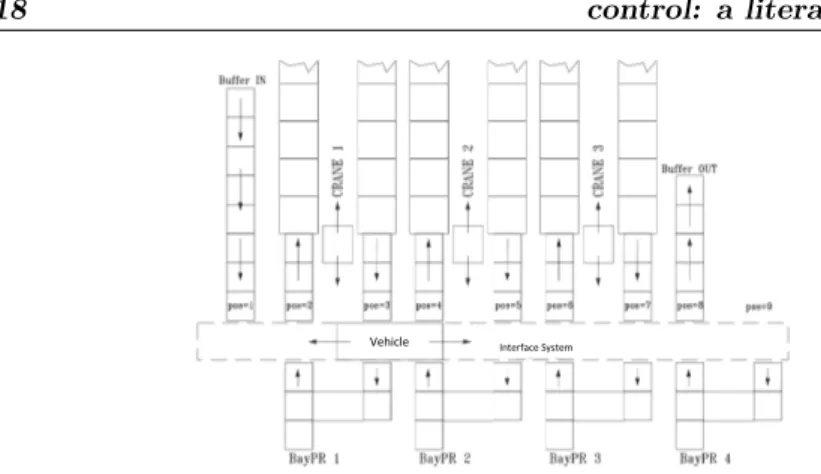
Since 1990 a big effort has been spent to find optimal strategies for planning and control of warehouse systems. Planning involves long-term optimization: it usually has a day or week time horizon and it is based on simplified models of warehouse systems and on statistical characterization of the system performance [Van99]. Conversely, a detailed model is used for the control which performs the short-term optimization of handling sequences, that usually has the objective to minimize the time to complete a little number of picking or storage operations and it is based on the current state of the system. A general warehouse architecture consists of a number of aisles, each one served by a crane, an Interface System (IS) and picking positions (see Fig. 3.1).

On both sides of each aisle there is a storage rack composed of nr rows and nk columns; moreover, as it has been said, each

aisle is served by a crane, capable of moving both vertically and horizontally at the same time, which performs the following oper-ations: i) picking of the Stock Unit (SU) at the input buffer/bay

(24)

18 control: a literature review

  

Figure 3.1 Scheme of a general warehouse architecture

of the aisle to be stored in a rack location S; ii) storage of the SU into the assigned location S of the rack; iii) movement to location R where a retrieval has been requested; iv) retrieval of the SU stored in R; v) movement to the output buffer/bay of the aisle to deposit the SU. This set of operations is called, in the warehouse system context, a Dual Command (DC) machine cycle [GHS77], [BW84], [HMSW87], [LdSO96]. The DC cycle can be generalized to the case of multiple storages and retrievals for cycle.

The IS consists of vehicles which can move a number of SUs. The vehicles move along a mono-dimensional guidepath placed orthogonally with respect to the aisle axis. They perform picking actions (from the aisles output bays and from the picking area output bays) and deposit actions (into the aisles input bays and into the picking area input bays).

The picking area represents the output point of warehouse sys-tems. A picking bay consists of a picking location connected via conveyors to the IS input and output interfaces, so that a SU can be partially emptied by a human operator and then carried back to an aisle rack location.

An input buffer represents the interface of the warehouse with the incoming area. It is used to load full SUs in the warehouse.

A set of missions is given as input to this kind of systems. Each mission requires that a certain quantity of an item, which can be stored in more than one aisle, is moved to a picking bay. Hence,

(25)

19

the execution of a mission requires the choice of the SU to move among those containing the desired item (this choice includes also the choice of the crane since there is one crane in each aisle), the choice of a vehicle to transfer the SU to the picking area, the choice of the picking bay, again the choice of a vehicle to return the SU in the storage area and the choice of the location where the SU must be stored among those available.

The control problem consists in assigning each available re-source (a location, a picking bay, a crane or a vehicle) to a mission. When one resource is available for a set of missions, a conflict oc-curs. The output of the control problem consists in determining Who has to do What and in Which Order in a manner that a certain objective is reached over a certain time horizon. In other words, the control must solve these conflicts. A detailed model is needed since it is important to detect in which order these conflicts occur.

This thesis focuses on how to obtain a model oriented to the control and to the performance analysis of these systems. In par-ticular, the complexity of modern warehouse systems, like the real one considered in Chapter 5, requires big interfaces (e.g. a carousel, shuttles, rail guided vehicles) between cranes and pick-ing area and so many vehicles must be used. Furthermore, when each crane cycle involves more than one picking and deposit, the number of SUs moved by vehicles at a time in the interface area grows, and then a significant time is required to cover the interface guidepath.

Discrete event systems have been proposed to obtain such a detailed model in [ABCC05] and in [DF05].

The challenging problem is the control of the IS since the con-trol of the cranes has been studied a lot in the literature. In a certain sense, the control of the whole warehouse reduces to that of the cranes if the time to cover the IS is negligible. In [ABCC05] it is shown that a key point in the development of the warehouse optimization is that the crane optimization can be considered inde-pendent of the vehicle optimization if a vehicle requires a negligible time with respect to the crane mean cycle time to reach the crane

(26)

bay from a picking bay. Thus, as soon as a cycle ends, a crane can start another cycle.

Once a crane cycle has been created (i.e. the list of locations to visit in a single travel to store and to pick SUs), the cycle time is deterministic and it can be analytically computed. In this disser-tation it is assumed that the cranes work according to an extended version of the algorithm presented by the authors in [ABCC05] to optimize DC cycles, but the effectiveness of the approach here presented is independent of the crane algorithm.

Note that cranes have not a discrete event behavior. The dis-crete event behavior of an automated warehouse is caused by the IS. The activity of the IS is more relevant when the number of vehi-cles and the number of interface bays grows, and consequently the stop and go state of the vehicles related to event occurrences grows (e.g. a collision of two vehicles must be avoided, a vehicle stops when it reaches a certain interface bay, etc.). This increases the time to move a SU from the picking area to the aisle input bays and reduces the crane performances independently of the crane optimization algorithm.

Moreover, when the size of the IS grows also its continuous time phenomena cannot be neglected. Indeed, a more precise informa-tion about vehicles posiinforma-tion becomes relevant. Using Petri Nets (PNs) [Mur89] a guidepath is represented by a number of places. These places model the presence of a vehicle in a certain zone of the IS. The exact position in this zone is unknown. A better precision requires many places. On the other hand, a continuous time system allows to represent the exact position as well as the mode changing in dynamics of vehicles (acceleration, deceleration or constant velocity).

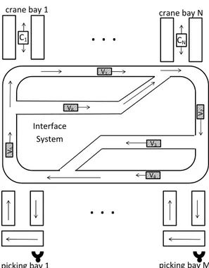
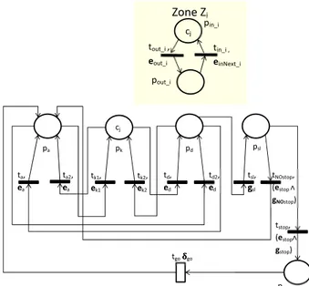
In this dissertation a particular warehouse layout is considered, presented in Fig. 3.2, where the interface system is made up of a circular path where vehicles continually turns transporting SUs. Indeed, during the researches made to write this thesis, it has been pointed out how such a layout is very common in several real warehouses (as the one presented in the case study).

(27)

21  



 _{}    ___             

Figure 3.2 Layout of a general real warehouse architecture: at the top aisles and crane bays (blocks C1. . . CN represent the cranes serving the

respective aisles), at the bottom picking bays, in the center Interface System routes with running vehicles (blocks Vi, with i = 1 . . . 6 represent the

(28)

formal model is presented. Two different approaches have been used: first a discrete event model based on the standard Colored Timed Petri Net (CTPN) [Jen95, HHC98] formalism is proposed, and then the same is obtained using Hybrid Petri Nets (HPNs) [DA01]. Difference between the two approaches is that in the first case both picking/crane bays and the IS have a discrete event dynamic and for this reason they are modeled as DESs; in the second case instead the IS is modeled as a continuous system.

The both models are highly modular, compact and made of pa-rameterized modules: the reuse of model components to model dif-ferent warehouse systems is very easy. In the both cases the overall system model is obtained by composing elementary modules ac-cording to the constraints [TTV06] represented by vehicles route. The interface with a higher level scheduler (dispatcher) is embod-ied in the obtained model, thus allowing off-line performance eval-uation of state-dependent dispatching control algorithms, as well as on-line implementation of complex control algorithms which are based on look-ahead (or what-if) techniques [HC99].

As more, the models of warehouse systems are used to obtain a deadlock prevention policy and to evaluate the systems perfor-mance via an experimental campaign based on simulations of a real case study in a very efficient way.

3.1 Warehouse Systems

A lot of results are available for unit-load automated storage sys-tems, while few results are available for other storage systems

[RRS+_{00, GGM10]. Moreover, there is an enormous gap between}

the published warehouse research results and the practice of de-sign and operations. As raised in [GGM10], a challenge for the research in this field is the integration of optimization, simulation and modeling of the full warehouse systems, not only automated storage and retrieval systems. One of the contributions of this dis-sertation is to show the importance of an accurate modeling and simulation of these systems. The optimization is not the topic of

(29)

3.1. Warehouse Systems 23

this thesis, but the experimental results presented in Chapter 5 show that it is greatly influenced by the model accuracy.

In [DF05] a unique model for automated storage and retrieval systems, comprising rail guided vehicles and narrow aisle cranes, is proposed. In the approach presented in this dissertation, differ-ently from [DF05] the activity of automated storage and retrieval subsystems reduces to a timed transition modeling the time to per-form a given cycle: the aisles and their locations are not explicitly modeled. This allows one to obtain a model of a reasonable size for real warehouses like the one considered in the following chapters. Model oriented to the control of an AS/RS system is presented

in [XWW+_{07]. Using P/T PN, the authors first obtain a model}

of the system layout, than they simplify it to have a model more convenient for analysis and simulation. Finally, colors and tempo-rized transitions are introduced to solve merging traffic problem of goods on conveyors. Colors are used to indicate the SUs destina-tions while time properly model temporized acdestina-tions, as the moving of a SU from a conveyor to another one, in this way a FIFO rule for the passage of SUs on the conveyors is implemented. Also in this thesis a simpler model of the system, called aggregate model (see Chapter 4, Section 4.2.14), is used to detect the possible presence of deadlocks, but differently from [XWW+_{07] deadlock prevention}

is carried out by means of an opportune resource allocation policy. In [HCL07] a modular CTPN model of an automated warehouse is presented. Each module describes a different action in the sys-tem (i.e. loading/unloading of a pallet on a crane, entering of a pallet in the warehouse...) and they can be composed to describe the warehouse overall behavior. Inhibitor arcs are used and a new kind of node is introduced, called virtual place, to accommodate instructions from schedulers (i.e. fixing destination of a pallet, what shuttle reserving for move the pallet...). The model is than implemented in a C++ code to simulate the system behavior. In the approach presented in this dissertation, neither inhibitor arcs nor virtual places are used. TPNs are used in [XH11] to model a logistic warehouse on the base of its operation procedure: the result is a modular model that can be used to simulate the flow

(30)

of the operations in the system. The model presented in this the-sis model both the logical operation procedure and the physical layout of the system.

Using commercial simulation tools like Arena$c _{or Automod}$c

is possible to model systems like the one presented in this thesis. However, they are not based on a formal model, and so, they are not enough general to be applied to every ISs. Moreover, they can be used only to simulation purposes, while a formal model allows to check system properties (e.g. deadlock avoidance) by formal analysis.

Among formal modeling methodologies, an appealing approach is the matrix-based framework proposed by [TL97]. Application to warehouse systems can be found in [GZNL08] where a variable dispatching rule control approach is used for operational control issues. In the same paper it is shown that the matrix-based model can be included into a multi-level control architecture where the model is used to determine when a control decision has to be taken from upper levels, and to feature operational control tasks too. Simulation is used to tune, off-line, some parameters of the control law. In this thesis, a similar approach is followed in a discrete as well as in a hybrid system context.

3.2 Deadlocks

Three basic approaches have been developed (see [FZ04] and the reference therein) for the deadlock resolution problem in auto-mated manufacturing approach, “deadlock detection and recov-ery”, “deadlock avoidance” and “deadlock prevention”. In the context of Interface Systems (ISs) “deadlock prevention” or “dead-lock avoidance” approaches must be used. Indeed, these systems have a very hight throughput and a deadlock recovery requires a too high price in terms of time and cost. The first one consists either to design a system such that deadlocks will never occur or to add a control mechanism on resource requests which prevents deadlocks to occur [HZL12]. The second one consists in using a

(31)

3.2. Deadlocks 25

real time deadlock controller to rule the resource assignment ap-plying look–ahead strategies.

An IS can be considered a simple guidepath-based traffic sys-tem [RR08], like Automated Guided Vehicle (AGV) or Rail Guided Vehicle (RGV) systems, since it consists of a number of vehicles that travel among a number of locations, following some prede-termined paths. However, links of this guidepath network are unidirectional, while in general case they are bi-directional; the motion of the vehicles on these links is unidirectional; vehicles can travel by following pre-specified routes in the guidepath network, while in general case they develop their route in real-time, based on the prevailing congestion conditions in the network; idle vehi-cles remain in the guidepath network during their idling period moving among various links, while in general case they are moved only to clear the way for some other vehicles or they will retire to a particular location of the guidepath network known as the sys-tem docking station. In [RR08] the problem of enforcing liveness for guidepath-based traffic systems is addressed in a discrete event context.

In [DF07] a deadlock avoidance policy is presented for a RGV system used to load/unload the automated warehouse where the picking area bay has infinite capacity, cranes have capacity one, and idle vehicles remain on the guidepath link until they receive a new mission.

The wrong management of the vehicles in ISs, when they re-main in the guidepath network during their idling period moving among various links, can afford a particular deadlock condition, called “livelock”: due to the bad vehicle assignment, picking and crane bays can become completely full. As consequence no more exchanges with the IS can occur. While in this condition the crane system is blocked (busy cranes are unable to unload the SUs on the bays and for this reason they are halted at the interface points), the IS is not: busy vehicles continue to run along the path, wait-ing for a free position on their bay destination. The system is not physically blocked, but no missions can be completed, energy is lost, and vehicles continue to run.

(32)

The problem of livelocks in the AGV systems in a discrete-event context with bidirectional guidepath network, unidirectional vehicles, zone control for avoiding collisions, and dynamic route planning is the topic of the preliminary paper [Ros02], and it has been generalized in [RR08]. As it has been explained before, ISs are simpler than AGV systems: there are not bidirectional paths and they do not have bridges between routes but (in case) only branches. Indeed, ISs are used to decouple the warehouse and the picking area to empty SUs as soon as possible, then the layout is chosen as simple as possible to make transport operations fast.

As for the blocking properties, another goal of this dissertation is to show that a livelock can occur in ISs. Moreover, it is proposed to achieve livelock-freeness enforcing policy by enforcing deadlock-freeness on a discrete event model properly obtained from the hybrid one.

(33)

Chapter 4 Warehouse system models

In this chapter two modular, compact, scalar approaches to model complex automated warehouse systems are presented.

First a discrete event model based on the standard Colored Timed Petri Net (CTPN) [Jen95, HHC98] formalism is proposed and then a hybrid model based on a new Petri net formalism that merges the concepts of Hybrid Petri Nets and Colored Petri Nets then is discussed. Both the models of the warehouse can be used for the performance evaluation as well as for online implementation of control algorithms.

4.1 Colored Timed Petri Net Model

In the next it will be show how the IS can be considered made up of several interacting modules, each one with own characteristics. To properly model each module, the concept of CTPN block is introduced:

Definition 4.1.1. A CTPN block is a tuple B = (C, Tin, Tout)

where C is a CTPN, Tin ⊂ T is the set of the input transitions,

Tout ⊂ T is the set of output transitions and Tin ∩ Tout = ∅.

Pre(p, t) and Post(p, t) matrices are diagonal matrices _{∀p ∈ P} and _{∀t ∈ T , i.e. firing of a transition t w.r.t. color c}h only

(34)

Input and output transitions allow connecting CTPN blocks together by means of dummy places. When M blocks are con-nected together a new CTNP block B! _{= (C}!_{, T}!

in, Tout! ) is obtained

where C! _{= (P}!_{, T}!_{, Pre}!_{, Post}!_{, Cl}!_{, Co}!_{) with P}! ₌. %M

i=1Pi

/ % D, where Pi=block i encapsulated net place set and D=set of dummy

places needed to link blocks together; T! ₌ %M

i=1Ti, where Ti=

block i encapsulated net transition set; Pre! and Post! are the new pre and post incidence matrices; Cl! =%M_i=1Cli, where Cli is

the block i encapsuled net color set; T!

in =

!

t : t _{∈ T}in,i,•t = ∅

" , with i = 1 . . . M and Tin,i=block i input transition set; Tout! =

!

t : t∈ Tout,i, t• =∅

"

, with i = 1 . . . M and Tout,i=block i output

transition set.

Ways to link blocks together are:

• “1 → 1” or sequence: given two blocks B1 = (C1, Tin,1, Tout,1)

and B2 = (C2, Tin,2, Tout,2) they are connected in 1→ 1 when

a dummy place d is added such that d _∈ •_t

in and d ∈ t•out,

with tin∈ Tin,2and tout ∈ Tout,1, Co(d) = Co(tout), Co(tin)⊆

Co(tout).

• “N → M” or hub: given N blocks Bj = (Cj, Tin,j, Tout,j),

with j = 1 . . . N , they are connected in N → M way to

the blocks Bi = (Ci, Tin,i, Tout,i), with i = 1 . . . M , when a

dummy place d is added such that d ∈ •_t

in,i and d∈ t•out,j,

with tin,i ∈ Tin,i and tout,j ∈ Tout,j, Co(d) = %N_j=1Co(tout,j).

If ∃(h, k) : h )= k, Co(tin,h) ∩ Co(tin,k) )= ∅ with tin,h ∈

Tin,h, tin,k ∈ Tin,k then a structural conflict between tin,h

and tin,k occurs. When N = 1, M > 1 hub connection is

called branch; if M = 1, N > 1 hub connection is called confluence.

For each connection presented above the following conditions have to be respected:

(i) %N_i=1Co(tin,i)⊆%Nj=1Co(tout,j);

(35)

4.1. Colored Timed Petri Net Model 29

(iii) Pre(d, t) (Post(d, t)) is a diagonal matrix; (iv) _|•_t

in,i| = 1 and |t•out,i| = 1.

Proposition 4.1.1. Connecting two or more CTPN blocks to-gether, no synchronization is introduced.

Proof. A synchronization may occur if |•_t_{| > 1 or Pre(p,t) is not}

a diagonal matrix (two tokes of different colors in the same input place are required to enable an output transition under a certain color).

Because of condition (iv), the first case (i.e. _|•_t_{| > 1) cannot}

occur.

When connection of M CTPN blocks is performed the resulting pre-incidence matrix is

Pre! = 0

Pre1 . . . Prei . . . PreM

Pre(D, T1) . . . Pre(D, Ti) . . . Pre(D, TM)

1

where Prei is the block i encapsuled net pre-incidence matrix,

Pre(D, Ti) is the weights matrix of the arcs connecting dummy

places with block i encapsuled net transitions. Since Prei(p, t)

is a diagonal matrix ∀p ∈ Pi, t ∈ Ti and since Pre(d, t) is a

diagonal matrix ∀d ∈ D, t ∈ Ti, Pre!(p, t) is still a diagonal

matrix _{∀p ∈ P}!_{, t}_{∈ T}!_.

4.1.1 CTPN Model of the IS

A IS consists of a unidirectional path along which vehicles move. This path, without loss of generality, can be divided in these basic components:

1. Elementary zone, where a unique route is possible and there are not interfaces with other subsystems.

2. Switching zone, where more than one route is possible since the path can branch off in different lines of travel.

3. Interface zone, where a vehicle stops to load (unload) a SU from (to) another subsystem bay.

(36)

1 0 0 1 1 0 p t ₁ t 2 ( c ₁_,1 ) ( c ₂_,1, c ₂_,2) ( c ₂) ( c 1 , c 2 ) (a) e ₁ p t 1 t 2 ( c ₁_,1 ) ( c ₂) (b)

Figure 4.1 (a) Marked CPN as seen in Chapter 2; (b) Marked CPN in (a) with simplified notation.

In this section it is shown how these components can be mod-eled each one by a single CTPN block, so the whole IS can be modeled by a CTPN obtained properly connecting a set of CTPN blocks. This formalism allows an easy conflicts detection and then it allows an easy implementation of the controllers based on patching rules. The output of dispatching rules actions is to dis-able all the events except one. Although such controllers produce only a locally optimal solution to the conflicts problem, they are simple to implement and they face the possible combinatorial ex-plosion of the control of the mission-to-resource-assignment prob-lem.

For the sake of simplicity, with reference to Chapter 2, some special notations are used to draw CTPNs:

• When transition occurrence colors can fire under any input place color, no colors are indicated at transition side [see Fig. 4.1(b)] for transition t2). If a transition occurrence color

can fire only under some specific input place colors, they will be indicated near the transition [see Fig. 4.1(b) for transition t1].

• If no matrix is indicated near an arc, an identity matrix I is intended to be associated to that arc [see Fig. 4.1(b); this is the case of the arc from place p to transition t2].

• eh near an arc from place pi to transition tj or viceversa

de-notes a column vector of size ui, with the h-th element equal

to one and the other elements equal to zero [see Fig. 4.1(b); this is the case of the arc from place p to transition t1].

(37)

4.1. Colored Timed Petri Net Model 31 



           (a) 



  (b)

Figure 4.2 Elementary zones module: (a) CTPN; (b) block representation.

Colors can be used to discriminate a free vehicle from a busy one, to identify where busy vehicles are directed and to identify a SU. SU identification is not essential in the IS since SUs are moved according to their destination in the IS path, but it is used to associate the crane location once a SU reaches a crane. For this reason, each net place has as many colors as the possible vehicles destinations plus one color that identifies an empty vehicle, but a SU number is associated to each token.

In real automated warehouses each zone can be occupied by just one vehicle at time: a vehicle has to halt while the next zone is busy.

Firing time of timed transitions depends on the length of the zone and represents the time necessary to the vehicle to cross the zone. For the sake of simplicity, in this first approach acceleration and deceleration have been neglected. Hence, vehicles can have only two speeds, v = 0 when they are stopped and v = Vmax when

they are moving. With these simplifications, a IS Elementary Zone (EZ) can be modeled like a “simple belt conveyor”. This technique simplifies also the modelling of interface zones since crane or pick-ing bays consist of belt conveyors.

In Fig. 4.2 the block representation of an EZ is shown: in Fig. 4.2(a) the CTPN model is visible, while in Fig. 4.2(b) the black-box version of the same is reported.

Switching Zones (SZs) can be modeled as shown in Fig. 4.3. Notice that a behavioral conflict occurs every time a token is present in the place P2 of Fig. 4.3(a), while a confluence is present

(38)



              (a)    



(b) 



           (c) 



   (d)

Figure 4.3 Switching zone: (a-b) output branch point and (c-d) input branch point .

In EZs and SZs the occurrence color of the firing output tran-sitions is the same of the firing input trantran-sitions, i.e. no transfor-mation color occur in the module.

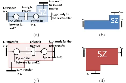
Interface Zones (IZs) between vehicles and crane (or picking) bays can be modeled as shown in Fig. 4.4. Dotted places Me and

Mf are not part of the modules but they are resource places needed

to model the conditions for enabling the SU exchange between picking bays and vehicles. As example, in Fig. 4.4(a) [Fig. 4.4(b)] exchange can occur only when transition tin2 (tout2) is enabled, i.e.

when a ce(ch)-color token is in resource Me (Mf), that model the

presence of a free (busy) vehicle in the IZ. When tin2 (tout2) fires,

a ch(ce)-color token is added in Me (Mf), modeling the new state

of the vehicle. After the adding of the new token, transition tout1

can fire and the token is passed in the next zone.

Unlike EZs and SZs, occurrence color of the IZs output transi-tion tout (tout1 for the IZ modeling passage from IS to the bay) can

be different from the occurrence color of the input transition tin1.

This occur as consequence of a change in the state of the vehicle (from busy to free and viceversa), when an exchange with the bay occurs.

(39)

4.1. Colored Timed Petri Net Model 33 



                           (a)     



(b) 



                         (c)   _   



(d)

Figure 4.4 Interface zone: (a-b) passage of SUs from bay to vehicle and (c-d) viceversa .

In the modules introduced above there are not synchronization, but only choices and confluences appear in SZs and IZs. As more, if only the skeleton of the nets are considered, without considering resources, it can be noted that the nets modeling each modules are State Machines. In the following the state machine definition and the liveness property are recalled.

Definition 4.1.2 (see [Mur89]). A State Machine (SM) is an or-dinary net such that each transition t has exactly one input place and one output place, i.e.,

∀t ∈ T,2

p∈P

Pre(p, t) =2

p∈P

Post(p, t) = 1.

Theorem 4.1.2 ([Mur89]). A state machine _{!N, m}0" is live iif

it is strongly connected and it has at least one token in its initial marking.

Modularity is an advantage of the CTPN model presented: it can be adapted at several layouts just adding or removing EZs; as

(40)

               (a)       





     _ 



       



  





           



 (b)

Figure 4.5 A possible IS layout; (a) physical layout and (b) its model.

more, if a new bay or a new route is added, it can be connected at the IS just introducing the CTPN module modeling an IZ or a SZ respectively.

As example, in Fig. 4.5(a) a possible layout is reported. Notice how it can be modeled in a very simple way, properly connecting 2 EZs, 2 IZs and 2 SZs, forming a closed path [Fig. 4.5(b)].

4.2 Colored Modified Hybrid Petri Net

Model

The previous CTPN model has been obtained looking to the ware-house system as if it is made up of only discrete event subsystem. However, when the spatial extension of this kind of systems grows, their continuous time behaviors cannot be neglected. Indeed, a more precise information about the position/state of the vehicles becomes relevant. As for example, using discrete event system formalism like PNs, a path is represented by a number of places. Such places model the presence of a vehicle in a certain zone. The

(41)

4.2. Colored Modified Hybrid Petri Net Model 35           

Figure 4.6 Mass system used in the example of section 4.2.2. exact position in the zone is unknown. A better precision requires many places. On the other hand, a continuous time system allows to represent the exact position but the mode changing in dynamic of vehicles (acceleration, deceleration or constant velocity) as well as the stop and go state of the vehicles (e.g. a vehicle stops when it reaches a certain position) would not be easily modeled. Then a possible solution is to use a hybrid model: this allows one to model picking and crane bays still as discrete event systems (in particu-lar like a sequence of belt conveyors) and, contemporaneously, to model the IS as a continuous system.

Before to present the hybrid model the Modified Colored Hy-brid Petri Net are introduced. An example is discussed in detail to motivate the introduction of the new formalism.

4.2.1 Colored Modified Hybrid Petri Nets

In this dissertation MHPNs where (2.8) is a linear function of m(τ) and u(τ) are presented. In this way, systems switching between several linear, time-invariant, continuous dynamics can be mod-eled. Moreover, to compact the state representation, a structured marking is used, as proposed in [GU98] and [CPV99]. In addition, for the whole net, colors are used to define a more compact model of the systems. This new kind of net is named Colored MHPN (CMHPN). Before giving its formal definition, the CMHPN for-malism is introduced by means of a motivation example.

4.2.2 Motivation Example

Consider two unitary masses moving, without friction, along a path with a uniformly accelerated linear motion, as shown in Fig.

(42)

                

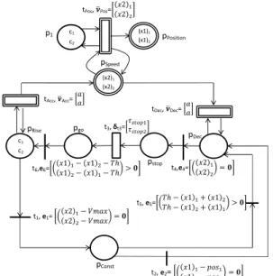
Figure 4.7 A MHPN model of mass i moving along a path.

4.6. Each mass state is described by position x1 and speed x2, related each other by the following equations:

' _˙ x1 ˙ x2 ( = ' 0 1 0 0 ( ' x1 x2 ( + ' 0 1 ( a (4.1)

where a is the constant acceleration. Assume the masses can ac-celerate until (Vmax− x2) = 0, and then, they continue to move

with constant speed, so (4.1) becomes:

' _˙ x1 ˙ x2 ( = ' 0 1 0 0 ( ' x1 Vmax ( (4.2) To avoid collisions, the masses regulate their speed in the man-ner that distance between them is equal or greater than a fixed threshold T h. Moreover, each mass has to start to decelerate if its position x1 is equal to a certain value posi. It decelerates until its

speed is zero, then it stays stopped for a time τstopi, and then it

starts to accelerate again only if the distance with the next mass is still greater than the threshold.

To model each mass behavior the modified HPN shown in Fig. 4.7 can be used: the marking of place pP ositon represents

the actual mass position, while the marking of place pSpeed

(43)

4.2. Colored Modified Hybrid Petri Net Model 37

the speed value is incremented (decremented) by transition tAcc

(tDec) with a firing speed just equal to the input value a. Position

depends on the firing speed of transition tP os, which is equal to

pSpeed marking. Note that when mpSpeed = 0, νP os = 0 and,

conse-quently, even if tP os is still enabled, it does not change mpP osition. Transition tAcc(tDec) can fire only when discrete place pRise (pDec)

is marked. Firing of discrete uncontrollable transition t1 (t2) is

associated to the internal condition e1 (e2) that is verified when

the vehicle reaches the maximum allowed speed value (the vehi-cle reaches a determinate position). When t1 fires, discrete place

pConst becomes marked: both tAcc and tDec are disabled,

conse-quently the marking of pSpeed remains constant (i.e. the vehicle

runs with constant speed). Uncontrollable discrete transition t4

fires when marking x2 is equal to zero (i.e. the vehicle is stopped):

in such a case a token is put in discrete place pStop, enabling

dis-crete timed transition t3. When a time equal to the firing delay

δt3 is expired, t3 fires, enabling tAcc (i.e. the vehicle starts to move

again).

The whole system is modeled replicating the net shown in

Fig. 4.7 for each mass. To have a more compact

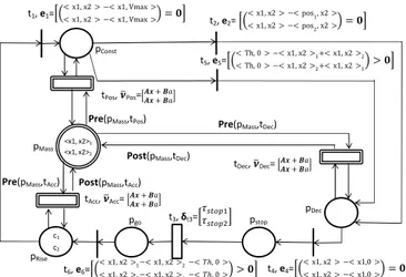
representa-tion colors, presented in [Jen95] and [HK98], are introduced in the HPN model. A different color is associated to each mass, so the system can be modeled with just one net that evolves w.r.t. two colors. For the sake of clarity, in Fig. 4.8 the marking of a discrete place w.r.t. the color i is indicated as ci; the marking of

the continuous places is indicated as (x1)i or (x2)i in the manner

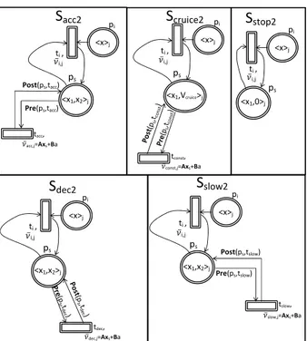
that its meaning is still obvious to the reader. Note that now firing speeds (both instantaneous and maximal), firing delays and logical expressions are column vectors, of dimension equal to the colors number. The i-th element of firing speeds (firing delays or logical expressions) vector associated to a continuous (discrete) transition is the firing speed (firing delay or logic expression) associated to the transition, w.r.t. the i-th color. Moreover, two new discrete uncontrollable transitions, t5 and t6, have been added compared

to the single mass model; these transitions manage the mass speed when the distance between the masses violates the threshold.

Issues in modelling and identification of Discrete Event Systems

































































Contents

Chapter 1

Preface

1.1

Thesis contribution

1.2

Thesis Overview

Chapter 2

Notations and Definitions

2.1

Petri Nets (PNs) and Colored Petri

Nets (CPNs)

2.2

Hybrid Petri Nets (HPNs)

Chapter 3

Issues about automated

warehouse system

modeling and control: a

literature review





3.1

Warehouse Systems

3.2

Deadlocks

Chapter 4

Warehouse system models

4.1

Colored Timed Petri Net Model

4.1.1

CTPN Model of the IS































