Production scheduling in pharmaceutical industry

(1)

UNIVERSITÀ DEGLI STUDI

TRE

Roma Tre University

Ph.D. in Computer Science and Automation

Production scheduling in

pharmaceutical industry

Luca Venditti

Advisor:

(2)

(3)

A thesis presented by Luca Venditti

in partial fulﬁllment of the requirements for the degree of Doctor of Philosophy

in Computer Science and Engineering Roma Tre University

Dept. of Computer Science and Automation 30 March 2010

(4)

Advisor:

Prof. Dario Pacciarelli Reviewers:

Prof. Alessandro Agnetis Prof. Rub´en Ruiz Garc`ıa

(5)

I would like to express ﬁrst of all my gratitude to Prof. Pacciarelli for his precious support and his constant helpfulness.

A particular thanks and aﬀective regards go to my PhD colleagues and all people that has taken part of AutOrI laboratory’s life during this years, from hard research activity to more recreational and relaxing moments.

(6)

Preface

Production scheduling is the phase of production management that produces a detailed description of operations to be executed in a given period of time, typically short. Production planning, instead, is characterized, compared to production scheduling, by an higher level of abstraction and a longer time pe-riod of interest. In most manufacturing systems the two main objectives to be achieved in production planning and scheduling are the maximization of the to-tal value produced by the plant and the on-time delivery of the final products. These two objectives are often in conflict with each other. Compared to other manufacturing processes, the pharmaceutical industry gives higher importance to on-time delivery over throughput maximization, due to the economical and legal implications of late deliveries and stock-outs at the final customers. Given the complexity of the production process and the issue of on-time de-livery, it’s difficult to have plans well balanced with the production capacity. In this contest, it is evident that scheduling is a critical operation and so, that an automated scheduling system is important, both to obtain good schedul-ing solutions and to have a better control of the production process. A first aim of this thesis is to give a demonstration of the improvements that may derive from an automated scheduling, by taking into account a real case study of production scheduling in a pharmaceutical industry, in the specific, in its Packaging department. At the same time, in this thesis, the issue concerning the difficulty of solving practical scheduling problems is arisen.

Besides operations management in a single stage, another interesting issue in production management, and in general for supply chain management, is the coordination between stages. In the last decades there is an increasing research activity on coordination of multiple decisions in supply chain man-agement as well as among diﬀerent stages of a production system. In the pharmaceutical supply chain, coordination issues are particularly important to

(7)

achieve the high standards of product quality and availability required by the legal and economical implications of product stock-outs at the final customers. Availability of final products requires not only to achieve excellence at each stage of the scheduling process but also in the coordination between different stages. A second aim of this thesis is to investigate on the benefits that the introduction of a centralized decision support system can bring respect to a de-centralized one; the case study of coordination between Packaging department and the subsequent Distribution stage of the pharmaceutical plant is addressed.

This thesis is organized as follows:

1. In Chapter 1 the production scheduling in the pharmaceutical industry is introduced, together with a description of common features in phar-maceutical manufacturing systems and of the the real plant considered 2. In Chapter 2 an overview of some academic problems that constitute a

basis for the resolution of real applications problems, is given. Classi-cal formulations of these problems, together with models and algorithms, found in literature, are ﬁrst presented; in a second analysis, some gener-alizations of classical formulations are considered, in order to gradually step, passing through more complex problems, into resolution of real ap-plication problems.

3. in Chapter 3 the ﬁrst case study, concerning scheduling of operations in the Packaging department, is shown. A detailed graph model and a Tabu Search algorithm are proposed

4. in Chapter 4 the second case study on coordination between Packaging and Distribution departments is presented. An extension of the graph model used in the previous case study and again a Tabu Search algorithm are proposed.

(8)

List of Tables

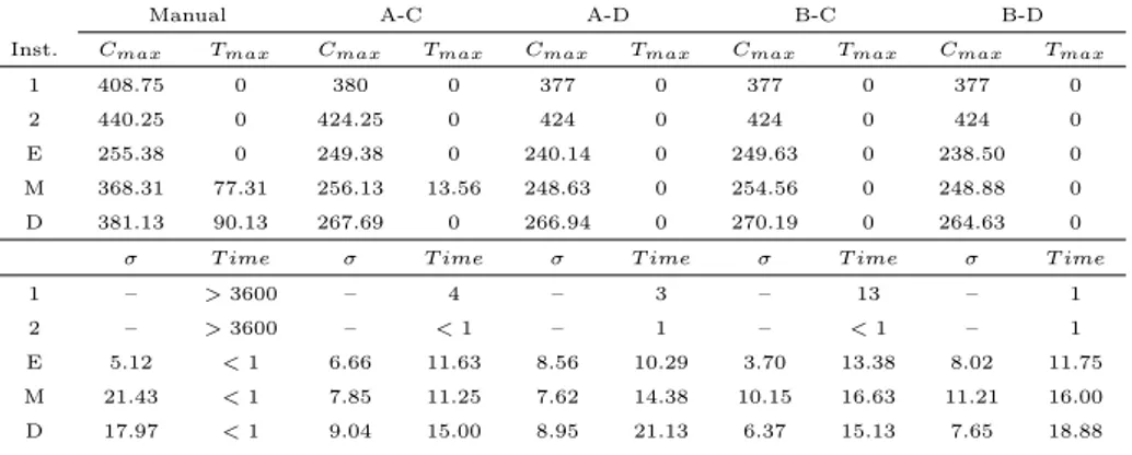
3.1 Comparison between manual and computerized schedules . . . 44

4.1 Test for decentralized approach . . . 62

4.2 Test for centralized approach . . . 62

4.3 Centralized approach with diﬀerent neighborhoods . . . 63

(11)

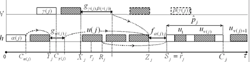
1.1 The pharmaceutical supply chain . . . 4 1.2 Typical layout of a secondary pharmaceutical manufacturing plant 5 3.1 Gantt chart for machines ℎ and ℎ′ and computation of 𝑆𝑗 . . . 30

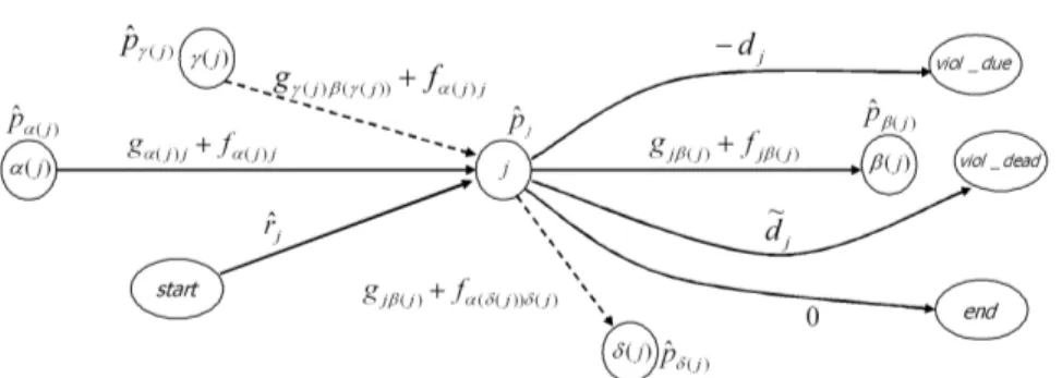
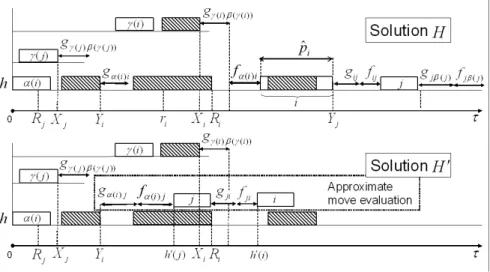
3.2 Node 𝑗 and weighted sequencing arcs in 𝒢(𝐻) . . . 32 3.3 Approximate evaluation of move 𝜑𝑀_{(𝑖, 𝑗). . . .} ₄₀

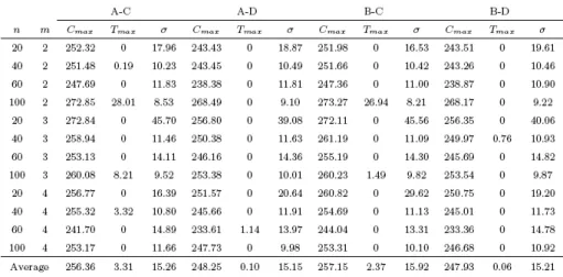
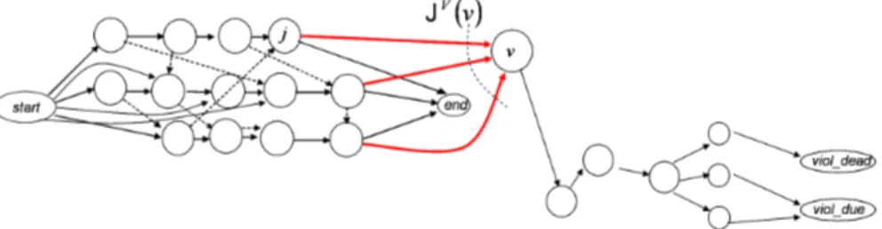
3.4 Performance of the tabu search algorithm for varying 𝑛 and 𝑚 . . 45 4.1 Graph model for the distribution problem . . . 53 4.2 Graph model for the centralized resolution approach for the

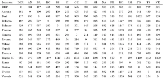
com-bined problem . . . 59 4.3 Distances between customer locations (km) . . . 61

(12)

Chapter 1 Production scheduling: the

pharmaceutical industry

Production scheduling is the phase of production management that produces a detailed description of operations to be executed in a given period of time, typi-cally short. This description contains, for each operation, the specification both of resources (machines, manpower, tools) to be used, and of time when they have to be executed. Production scheduling is often cited in combination with production planning, that is characterized, compared to production schedul-ing, by an higher level of abstraction and a longer time period of interest. In fact production planning has the aim of defining the orders to be produced in a medium or long term; the result of the production planning constitute constraints to be respected by the scheduling phase. In most manufacturing systems the two main objectives to be achieved in production planning and scheduling are the maximization of the total value produced by the plant and the on-time delivery of the final products. These two objectives are often in conflict with each other. In fact, the former requires the organization of pro-duction schedules with large lots, to reduce the number of setups and idle time; instead, for the latter objective an organization with small lots is preferable, with consequent increase of the number of setups and idle time and reduc-tion of the factory throughput. Compared to other manufacturing processes, the pharmaceutical industry gives higher importance to on-time delivery over throughput maximization, due to the economical and legal implications of late deliveries and stock-outs at the final customers.

In the pharmaceutical industry, production planning and scheduling usually

(13)

teracts as an open loop control chain, in which the planning phase determines input data and constraints to be satisfied by the scheduling phase. In the plan-ning phase, decisions are taken with the aim to satisfy the demand, that is not completely known at the moment of decisions. Then, in the scheduling phase, decisions have to be taken facing two kinds of constraints, i.e. the production orders released by the planning stage (in term of release and due dates) and the availability of the production resources. Hence, when the resource amount required by the plan is not sustainable by the available capacity, the schedule cannot comply with the plan, causing delays in the delivery of final products. So it is important that the production planned does not exceed the capacity of the factory. We have already stated the production planning is driven by the demand. This demand takes the form of wholesaler orders that are typically the result of a negotiation in which order quantities, due dates and penalties for late delivery are regulated by contracts. Contracts stipulations should take into account also future production capacity and evaluate the impact of new order on due dates of those currently in the system, in order to choose sustainable quantities and due dates. However, it is not easy to do this for various reasons, as the complexity of manufacturing processes (given among other factors by constraints related to contamination problems) or the issue of on-time delivery. In fact, these factors lead to frequent under-utilization of shop resources and disregarding of long-term due dates. As in a vicious circle, this difficulty in estimating reliable delivery dates to negotiate with the wholesalers, may cause frequent urgent orders, which further increase the short-term pressure on the operations managers. Given the complexity of the production process and the difficulty to have plans well balanced with the production capacity, scheduling is a critical operation in pharmaceutical industry. So, the importance of an automated scheduling system is evident, both for obtaining good scheduling solutions and for having a better control of the production process.

The remainder of this chapter presents, in Section 1.1, a description of common features in pharmaceutical manufacturing systems; then, a description of the real plant object of the case studies of this thesis, is given in Section 1.2.

1.1 Pharmaceutical manufacturing systems

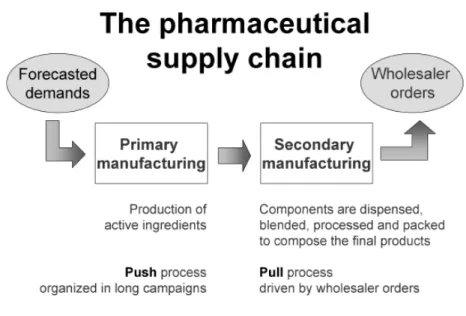
Typical pharmaceutical supply chain (Figure 1.1) contains at least two stages: primary and secondary manufacturing [10, 49]. The former is dedicated to the production of active ingredients and other basic components through complex chemical and biochemical processes. Production is typically a push process,

(14)

CHAPTER 1. PRODUCTION SCHEDULING: THE PHARMACEUTICAL

INDUSTRY 3

i.e. operations are pushed to next level whether needed or not, and it is orga-nized in long campaigns, to reduce the impact of long cleaning and setup times that are necessary to ensure quality and avoid cross-contamination. Primary manufacturing is therefore not very sensitive to short-term demand fluctua-tion, and the main issue here is a careful lot sizing to avoid shortages of active ingredients.Secondary manufacturing is usually a pull process, driven by whole-saler orders, in which active ingredients and other components are dispensed, blended, processed and packed to produce the final products. Secondary phar-maceutical manufacturing systems consist of a set of multi-purpose production facilities that produce a variety of intermediate and finished products through multi-stage production processes. Facilities are linked by supplier-customer re-lations, i.e., one facility produces intermediate goods that are processed further by other facilities, reflecting the material flow relationships given by the recipes of the final products. Furthermore, each facility may interact with external en-tities (e.g. suppliers) and/or internal ones (e.g. warehouses). For example, the area of interest for this thesis, i.e. the packaging area, is the one mostly con-nected to external entities.Primary and secondary manufacturing are typically decoupled by relatively large stocks of components.

From the point of view of production scheduling, it is more interesting to focus on secondary manufacturing only, because at this stage, scheduling is a critical issues to guarantee 100% availability of ﬁnal products at sustainable costs. In particular, the impact of a late delivery can be minor, as when the delay is absorbed by the wholesaler inventory system, or major, when it may cause a stock-out at ﬁnal customers. In the latter case, a hard deadline is associated to the product besides the due date.

Common production processes are devoted to producing solid, liquid, aerosol or powdered items according to a family of similar recipes [10]. For example, one of the main process families is devoted to Solid Dosage Manufacturing (SDM), which includes, among others, the production of tablets. Each com-mon production process consists of a set of self-contained activities.

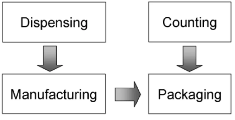
Hence, the production is typically organized with four main departments (with eventually a ﬁfth, the Distribution), as in Figure 1.2 which to a certain extent can operate independently of each other:

∙ Dispensing, where, with respect to the receipt, the availability of all materials required is checked (raw material handling) and materials are weighed and stored in sealed bins (dispensing).

(15)

Figure 1.1: The pharmaceutical supply chain

∙ Manufacturing, where most of activities are performed, i.e.: specific agents are prepared to be used together to wet powders in the granu-lation (binder preparation); then, dry materials from the bins are passed into a granulator and mixed with specific quantities of binder agents to produce, after a drying procedure, granules (granulation), that are then stored in bins; bin contents are then blended with, eventually, the addi-tion of new materials (blending); then granules are compressed in tablet presses (compression); finally, a solution is prepared and sprayed over the tablets (coating)

∙ Counting, where packages are prepared according to the diﬀerent orders and market places (counting)

∙ Packaging, in which tablets are put into packages to form the ﬁnal (or semi-ﬁnal, if they are sent in bulk packages to other sites) products (pack-aging);

(16)

INDUSTRY 5

Figure 1.2: Typical layout of a secondary pharmaceutical manufacturing plant

∙ Distribution, that constitute the ﬁnal stage, where ﬁnal products are delivered to customers.

Quality assurance and control activities are distributed throughout the whole manufacturing process. Dispensing and Manufacturing, as Counting and Packaging, are typically decoupled by means of the sealed bins where tablets are typically stored. When counting activities require a significant amount of work, counting and packaging are performed in different departments. This is a common situation in Europe, where the many different national regulations and languages require the handling of a huge number of different packages in the same plant [10, 39, 49].

Some common features of all departments are:

1. single-product processing, i.e. one product at a time is processed in the department (or in one of its rooms if there are more than one) to avoid cross-contamination between diﬀerent kinds of products;

2. cleaning operations, that are executed when switching from one prod-uct to another with the aim, again, to avoid cross-contamination; minor cleaning is suﬃcient when two consecutive products belong to the same family, i.e. they need, or they are composed (relating to tablets), by

(17)

com-patible raw materials; major cleaning is necessary when the raw materials are incompatible.

3. resource constraints, that limit the number of resources that can be em-ployed for a speciﬁc activity at any time. For example, manpower re-sources are categorized by their respective skills and low skilled operators can perform only a subset of simple tasks. This fact may limit, for exam-ple, the number of tool changes that can be performed simultaneously in a shift, when these activities involve complex mechanical operations. 4. sequencing constraints, that specify a partial ordering among the

opera-tions for a set of tasks. These constraints are typically dictated by each specific recipe, but sequencing constraints may be required also by the production process, by quality control or by specific management poli-cies. For example, in some cases a task can be started only after some equipment preventive maintenance or calibration task is finished. These features require incorporation of a number of relevant details into the scheduling models. For example, when switching from a product to an-other, it may be necessary to clean a machine and to change some tools, which involve mechanical operations. While cleaning operations can be performed by low skilled operators, mechanical operations require specialized operators. Moreover, different mechanical operations can be performed in parallel, and therefore a careful model of the setup time should take into account the num-ber of operators involved and their respective skills, besides the possible need for minor/major cleaning. Constraints may derive from specific plant manage-ment policies. For example, a departmanage-ment may prefer to organize production such that the starting/completion time of some particular operation is aligned with the beginning or end of a shift. Other departments may constrain each setup operation to be completely executed within the same shift, although there are no specific technological reasons for such requirement.

All these factors conﬁrm the need of a scheduling decision support system (DSS) to increase the eﬃciency of the factory by optimizing the use of resources and monitoring the production process to be able to give a quick response to changes that can occur.

(18)

INDUSTRY 7

1.2 An example of pharmaceutical plant

In this section we describe the plant object of study in this thesis, and in par-ticular the Packaging and Distribution areas. A more complete description of the plant and of the automated scheduling project for the whole plant can be found in [38]. The plant is located in Italy and it supplies different European countries. The production flow is organized into the four main phases described above. However, while there are only one dispensing and one counting depart-ment in the plant, manufacturing and packaging activities are organized with several departments. The production planning of the plant follows a 4-week rolling horizon strategy in which departments are called to solve their specific scheduling problems. The result of the planning is a set of production orders and a set of due dates for the final products to be delivered in weeks 3 and 4. These become due dates for the packaging department, which are propa-gated backward to the counting and manufacturing departments, by assuming approximately one week of lead time for each product, and to the dispens-ing department, by assumdispens-ing approximately two weeks of lead time for each product. At the beginning of week 1, the dispensing department schedules the production orders for weeks 1 and 2 and implements the schedule for week 1. If some products are delivered late with respect to the due dates defined by the plan, their scheduled delivery time are used as release times for the subsequent department. At the beginning of week 2, the manufacturing and counting departments schedule the production orders for weeks 2 and 3 and implement the schedule for week 2. Similarly, at the beginning of week 3 the packaging department schedules the production orders for weeks 3 and 4 and implements the schedule for week 3. The whole process is repeated every week, i.e., every week each department schedules the production for the next two weeks, to consider possible changes that may occur. For example, at the end of each week there may be production orders in some department that have not been delivered on schedule, or the production of one or more urgent orders is required by the planner, e.g., in case of stock-outs for some products. In such cases it may be necessary to re-schedule the production in different depart-ments, since late deliveries at a department may cause lack of materials at the subsequent department, while urgent orders cause extra requirements at the corresponding department. Late and urgent orders are managed as orders with strict deadlines to be processed as soon as possible. Clearly, deadlines make it difficult to organize long campaigns, and thus reduce the actual capacity of the departments. This reduction may cause, in turn, late deliveries at the end of the week and such negative effects may propagate over several weeks.

(19)

Packaging and Distribution

The Packaging department contains three packaging lines working in parallel. Each line can process one lot of identical products at a time and performs all operations from the production of blisters to the final individual specific packages. The number of lots per week processed by the packaging department is usually much larger than for the manufacturing department. In fact, for example, a single lot of tablets can be divided into many different lots of final products, differing from each other only in the package (corresponding for example to different countries)

Lines are multi-purpose, i.e. they can process more families of products with supplementary tools. However, not all lines can use a speciﬁc tool, so lines can process only some families of products. Tools are shared among families of similar products and available in a limited number of copies, in most cases there is a single copy of each tool. In each line, sequence-dependent setup and removal times occur before and after the processing of a lot, in order to clean and calibrate the line and to change the tool. A setup or removal time is called minor when requiring no tool change and major in the latter case. Lines can be unavailable in given periods for preventive maintenance operations.

Cleaning operations, mechanical configurations and lot processing require a given amount of work for human operators, therefore lines cannot process lots nor execute setups or removals without human resources. The same number of operators is required by each production line. Human resources availabil-ity is constant within a shift, but it can vary from one shift to another, the night shift being typically less supervised. In order to reduce the risk of cross-contaminations, the plant policy is to assign each operator to a specific line during the whole shift. Setups and removals cannot be interrupted while the processing of a lot on a line can be interrupted and resumed later on the same line if the line becomes unavailable for planned maintenance or if the number of operators in the subsequent shift is not sufficient to process the lot.

The Distribution department is the ﬁnal department of the chain. Resources are constituted by vehicles and operators. All vehicles have the same capacity and can contains every kind of package produced. Operators can be divided into internal operators, responsible for the freight of vehicles, and drivers. Deliveries are usually made during the day, except in some cases of urgent orders, in which they are made in the night.

(20)

Chapter 2 Literature on scheduling

problems: from theory to

practice

Models and algorithms known in literature are usually developed for solving simplified versions of real application scheduling problems. However they con-stitute a basis for the resolution of real world problems, that need more detailed models and more sophisticated algorithms to be faced. Some extensions of most known problems are considered in this chapter together with their models and some neighborhood definitions for Tabu Search, that can be taken as example of effective algorithm to solve practical problems.

2.1 Introduction

Most optimization algorithms from the scheduling literature are mainly con-cerned with the computation of optimal or near-optimal solutions to very sim-pliﬁed problems [40, 45]. According to the survey of Reisman, Kumar, and Motwani [42], out of 170 articles (related to ﬂowshop scheduling/sequencing) published from 1952 to 1994 only 5 were judged to be true applications. On the other hand, in the last years an increasing number of articles focus on re-alistic scheduling models including more practical constraints than in the past [37, 41, 45]. In this chapter we give an overview of some academic problems that constitute a basis for the resolution of real applications problems. Classi-cal formulations of these problems, together with models and algorithms, found

(21)

in literature, are ﬁrst presented; in a second analysis, some generalizations of classic formulations are considered, in order to gradually step, passing through more complex problems, into resolution of real application problems. Concern-ing with algorithms, only heuristics has been considered, because to consider exact algorithms would have gone out of the aim this thesis. In particular, tabu search algorithm and related neighborhoods are treated, because it is cer-tainly among the most successful heuristics for a large number of theoretical and practical scheduling problems [33] and it has been chosen for solving the two case studies in the this thesis. Among books on scheduling theory, in our review, we mostly refer to the classiﬁcation proposed by Brucker in [5] and by Brucker and Knust in [7].

The remainder of this chapter is structured as follows. In Section 2.2 some basic deﬁnitions for scheduling problems are given. Then, Tabu Search algo-rithm is described in Section 2.3. In Section 2.4 we introduce shop problems, that represent the most common environments in manufacturing scheduling. Some generalizations of shop problems are considered in Section 2.5. Finally, in Section 2.6 we introduce another class of problems adapt to represent real application scheduling, the multi-resource constrained scheduling problems.

2.2 Basic deﬁnitions

A schedule is an allocation of resources in one or more time intervals to activ-ities to be executed: a scheduling problem consists in ﬁnding a schedule such that some constraints are satisﬁed and some criteria are optimized (objective function). Usually, term machine is used to indicate the generic resource while the term task or operation is used to indicate an activity. A job is a set of tasks technologically related to each other.

Denoted with 𝐽𝑗 a generic job and with 𝑂1𝑗, . . . , 𝑂𝑛𝑗𝑗 its set of tasks, a job

is usually characterized by the following elements:

∙ a processing time 𝑝𝑖𝑗 required to process task 𝑖 of job 𝐽𝑗

∙ a set of eligible machines ℳ𝑖𝑗 for task 𝑂𝑖𝑗

∙ a release date 𝑟𝑗 indicating the time when the ﬁrst task of job 𝐽𝑗 is

available for processing

(22)

CHAPTER 2. LITERATURE ON SCHEDULING PROBLEMS: FROM

THEORY TO PRACTICE 11

∙ a deadline 𝐷𝑗 within which job 𝐽𝑗 must be completed

Classes of scheduling problems are specified in terms of a three-field classi-fication 𝛼∣𝛽∣𝛾, introduced by Graham et al. [20], where:

∙ the ﬁrst ﬁeld 𝛼 represents the shop environment. Some examples are sin-gle machine (indicated with 1), parallel machines (𝑃 ) and multi-purpose machines (MPM);

∙ the second ﬁeld represents the constraints of the problem. Some exam-ples are release times (𝑟𝑖), due dates (𝑑𝑖), deadlines (𝐷𝑖), precedence

constraints (𝑝𝑟𝑒𝑐), preemption (𝑝𝑚𝑡𝑛), sequence dependent setup times (𝑆𝑠𝑑) and resource unavailability (𝑢𝑛𝑎𝑣𝑎𝑙𝑗);

∙ the third ﬁeld represents the optimality criteria of the problem. Some examples are: makespan (𝐶𝑚𝑎𝑥), i.e. the maximum value, among all

jobs, of their completion times 𝐶𝑗; maximum lateness (𝐿𝑚𝑎𝑥), i.e. the

maximum value, among all jobs, of 𝐶𝑗− 𝑑𝑗; maximum tardiness (𝑇𝑚𝑎𝑥),

i.e the maximum positive value, among all jobs, of 𝐶𝑗− 𝑑𝑗; total

comple-tion time (∑𝑛

1𝐶𝑗), i.e. the sum of completion times of jobs. Optimality

criteria may be more than one (multi-criteria or multi-objective prob-lems); in this case a priority may be given to a criterion rather than to another (for example 𝐿𝑒𝑥(𝐶𝑚𝑎𝑥, 𝑇𝑚𝑎𝑥) indicates the minimization of the

two objectives in the lexicographic order)

2.3 Tabu Search

Among the most eﬀective algorithms for solving practical scheduling problems there is Tabu Search algorithm, that is an evolution of Local Search algorithm. Local Search is an algorithm that, given a solution, searches for better solu-tions among those near to the given one. This set of near solusolu-tions is obtained by applying an operator (move) to the current solution and it is called neigh-borhood ; when the neighneigh-borhood does not contains better solutions than the current one, the algorithm stops. The current solution is called local optimum. Tabu Search is a local search algorithm which makes extensive use of mem-ory for guiding the search. It takes its origins from ideas of Glover [15, 16] stimulated by the need for overcoming limits of Local Search, in which the exploration of the solution space is bounded by feasibility and local optimal-ity criteria. The key concept at the basis of Tabu Search, in fact, is that an

(23)

optimization algorithm, in order to be effective and efficient, must provide a large exploration of solutions but at the same time this exploration must be dynamically guided in an intelligent way that can be represented by two as-pects: a memory of the past exploration (adaptive memory) and the ability to change strategy during the exploration (responsive exploration).In particular, the adaptive memory is the main feature of Tabu Search together with the neighborhood. The information stored in this memory is used to modify the neighborhood 𝑁 (𝑥) of the current solution 𝑥 to obtain a new neighborhood 𝑁∗(𝑥) that is used for the exploration. The term adaptive memory can refers to various forms of memory introduced over the years with the development of more sophisticated tabu search procedures. This memory can be explicit, when the entire solutions are stored, or implicit, when solution attributes changed in the recent past, usually the moves performed, are stored. A first classification in this variety can be made, for example, between short term and long term memory. A short term memory is usually an implicit memory where only in-formation on the recent past of the exploration is available and typically this information is used to determine elements that have to be excluded from 𝑁 (𝑥) to obtain 𝑁∗(𝑥), that consequently is a subset of 𝑁 (𝑥). In a long term mem-ory, instead, information on a more ancient past of the exploration is available and typically this information is used to include additional elements in 𝑁∗(𝑥) together with elements of 𝑁 (𝑥). However, when we deal with Tabu Search in its basic scheme, we commonly refer to a short term memory, called tabu list, that keeps track of last solution explored during the recent past by storing the opposites of moves performed. A simple mechanism, combining the use of tabu list with the permission to explore non-improving solutions, gives the possibility to escape from local optima. In fact, if the current solution is a local optima the best non-improving solution can be selected as the new incumbent. At the next iteration, in a memory-less algorithm, optimality criteria would cause the algorithm to re-visit the last local optimum, thus establishing a cy-cle in the execution of the algorithm. This can be avoided by considering for the exploration the modified neighborhood 𝑁∗(𝑥) in which the last solutions visited are excluded. However, this mechanism does not guarantee the escape from local optima in any case. Problems are related to the tabu list length. In fact tabu list is a first-in first-out list, so a move is kept in it for a number of iterations equal to the tabu list size so in some cases this number may be not sufficiently high to avoid the algorithm to return to the last local optimum vis-ited. To face this problem more advanced algorithms feature a dynamic tabu list size. Another problem may arise when a solution obtainable with a tabu move is better than the best solution known at the current iteration; in this

(24)

case the move can be deleted from the tabu list and the corresponding solution mantained in 𝑁∗(𝑥). In general, criteria used to delete a move from the tabu list are called aspiration criteria.

Concerning to long term memory, its most common use consists in storing se-lected elite solutions, i.e. high quality local optima; for this reason long term memory is usually explicit. These solutions are typically involved in responsive exploration strategies as diversification and intensification. Intensification con-sists in exploring regions of the solution space that are considered particularly good, while diversification aims to explore unvisited regions. These regions are reached by moving the search to new solutions obtained from selected elite solu-tions; specifically, in the case of intensification strategy, selected elite solutions with similar components are assembled together to form new solutions, while in the case of diversification strategy, elite solutions with different features are combined.

Examples in the literature of sophisticated TS schemes for scheduling problems are [13, 36].

2.4 Shop scheduling problems

In this section we discuss shop scheduling problems, such as open shop prob-lems, ﬂow shop probprob-lems, job shop probprob-lems, and mixed shop probprob-lems, which are widely used for modeling industrial production processes. All of these prob-lems are special cases of the general shop problem, deﬁned in the following.

A set ℳ of 𝑚 machines 𝑀1, . . . , 𝑀𝑚 and a set 𝒥 of 𝑛 jobs 𝐽𝑗 with 𝑗 =

1, . . . , 𝑛 are given. Job 𝐽𝑗 consists of 𝑛𝑗 operations 𝑂𝑖𝑗 with 𝑖 = 1, . . . , 𝑛𝑗

with processing times 𝑝𝑖𝑗. Each operation 𝑂𝑖𝑗 must be processed on a machine

𝜇𝑖𝑗 ∈ ℳ. There may be precedence relations between the operations of all

jobs. Each job can only be processed by one machine at a time and each machine can only process one job at a time. The objective is to ﬁnd a feasible schedule that minimizes some objective function of the completion times 𝐶𝑗 of

the jobs 𝑗 = 1, . . . , 𝑛. The objective functions are assumed to be regular, i.e. non-decreasing functions of 𝐶𝑗

Job shop

The Job Shop Scheduling Problem (JSSP or Job-Shop) is one of the most studied combinatorial optimization problems in literature. The classic job-shop scheduling problem may be formulated as follows. A set ℳ of 𝑚 machines

(25)

𝑀1, . . . , 𝑀𝑚 and a set 𝒥 of 𝑛 jobs 𝐽1, . . . , 𝐽𝑛 are given. Job 𝐽𝑗 consists of 𝑛𝑗

operations 𝑂𝑖𝑗 with 𝑖 = 1, . . . , 𝑛𝑗 which have to be processed in the order

𝑂1𝑗 → 𝑂2𝑗, . . . , 𝑂𝑛𝑗𝑗. Operation 𝑂𝑖𝑗 must be processed for a processing time

𝑝𝑖𝑗 > 0 on a dedicated machine 𝜇𝑖𝑗 ∈ 𝑀1, ..., 𝑀𝑚. Each machine can process

only one job at a time and 𝜇𝑖𝑗 ∕= 𝜇𝑖+1,𝑗for all 𝑗 = 1, . . . , 𝑛 and 𝑖 = 1, . . . , 𝑛𝑗−1,

i.e. no two subsequent operations of a job are processed on the same machine (otherwise the two operations may be replaced by one operation). Such a job-shop is also called a job-shop without machine repetition. In the classic formulation there is sufficient buffer space between the machines to store a job if it finishes on one machine and the next machine is still occupied by another job. A schedule is defined by the vector 𝑆 = (𝑆𝑖𝑗) of the starting times of

all operations 𝑂𝑖𝑗. A schedule 𝑆 is feasible if: (i) 𝑆𝑖𝑗 + 𝑝𝑖𝑗 ≤ 𝑆𝑖+1,𝑗 for all

operations (precedence constraints between operations of the same job), and (ii) 𝑆𝑖𝑗+ 𝑝𝑖𝑗≤ 𝑆𝑢𝑣 or 𝑆𝑢𝑣+ 𝑝𝑢𝑣≤ 𝑆𝑖𝑗 for all pairs 𝑂𝑖𝑗, 𝑂𝑢𝑣 of operations with

𝜇𝑖𝑗 = 𝜇𝑢𝑣, (each machine processes only one job at a time). The objective is

to determine a feasible schedule 𝑆 such that the makespan 𝐶𝑚𝑎𝑥= max𝑛𝑗=1𝐶𝑗,

where 𝐶𝑗 = 𝑆𝑛𝑗,𝑗+ 𝑝𝑛𝑗,𝑗 is the completion time of job 𝐽𝑗.

A feasible schedule 𝑆 deﬁnes for each machine 𝑀𝑘 a sequencing 𝜋𝑘 =

(𝜋𝑘(1), . . . , 𝜋𝑘(𝑚𝑘)) of the 𝑚𝑘 operations that has to be processed on 𝑀𝑘.

Model

A job shop can be represented by a so-called disjunctive graph, introduced by Roy and Sussman in 1964 [43]. A disjunctive graph 𝒢 = (𝑉, 𝐶, 𝐷) is a mixed graph where 𝑉 is the set of nodes, 𝐶 a set of directed arcs (conjunctions) and 𝐷 a set of undirected arcs (disjunctions). In our case each node in 𝑉 represents an operation (including two dummy operations 𝑠𝑡𝑎𝑟𝑡 and 𝑒𝑛𝑑, one preceding and one following all operations. each arc in 𝐶 represents a precedence con-straint between two consecutive operations of the same job; ﬁnally, for each pair of operations which have to be processed on the same machine, there is an undirected arc in 𝐷 representing the two possible precedence relations be-tween the two operations. Nodes in 𝑉 are weighted with the processing time of corresponding operations. For ease of notation operations can be indicated with index 𝑖, the corresponding job with 𝐽 (𝑖) and the corresponding machine with 𝜇(𝑖), with 𝑖 = 1, . . . , 𝑛𝑜, with 𝑛𝑜 being the number of operations.

With the disjunctive graph representation, the problem of finding a feasible schedule for the job-shop problem is equivalent to the problem of fixing a direction for each disjunction such that the corresponding graph is acyclic. A set 𝒮 of fixed disjunctions is called a selection. A selection 𝒮 is called complete

(26)

if a direction has been ﬁxed for each disjunction in 𝐷; moreover, 𝒮 is called consistent if the corresponding graph 𝒢(𝒮) = (𝑉, 𝐶 ∪ 𝒮) is acyclic. Given a complete consistent selection 𝒮, a corresponding feasible earliest start schedule can be easily calculated. Denoted with 𝑟𝑖 the length of a longest path from

𝑠𝑡𝑎𝑟𝑡 to 𝑖 in 𝒢(𝒮), where the length of a path is deﬁned as the sum of the weights of all nodes on the path, node 𝑖 excluded, this feasible earliest start schedule can be calculated by setting 𝑆𝑖= 𝑟𝑖. Therefore, makespan 𝐶𝑚𝑎𝑥(𝑆) of

schedule 𝑆 is equal to the length 𝑟𝑒𝑛𝑑of a longest path from 𝑠𝑡𝑎𝑟𝑡 to 𝑒𝑛𝑑. Vice

versa, for each schedule 𝑆, there is an associated complete consistent selection 𝒮; the feasible earliest start schedule corresponding to 𝒮 is not worse than 𝑆 in terms of a regular objective functions, so only complete consistent selections may be considered.

Heuristic and meta-heuristics: local search and tabu search

Among the most effective algorithms for solving JSSP there is Tabu Search algorithm. Some definitions of problem-specific neighborhoods for local and tabu search algorithms based on the disjunctive graph are presented next. We have stated that only complete consistent selections may be considered. A natural way to go from one complete selection 𝒮 to another selection 𝒮′ is to reverse certain disjunctive arcs. A first neighborhood 𝑁𝑐𝑎, introduced by

van Laarhoven et al. [52] may be deﬁned by reversing critical arcs. In fact, as they observed, re-sequencing consecutive jobs that are not on the longest path from 𝑠𝑡𝑎𝑟𝑡 to 𝑒𝑛𝑑 cannot improve the makespan. More speciﬁcally, a neighbor in 𝑁𝑐𝑎(𝒮) is generated by a move that reverses one oriented disjunctive arc

(𝑖, 𝑗) ∈ 𝒮 on some critical path in 𝒢(𝒮) into the arc (𝑗, 𝑖). This neighborhood has the property that all selections 𝒮′∈ 𝑁𝑐𝑎(𝒮) are feasible. This can be proved

as follows. Assume to the contrary that a selection 𝒮′ ∈ 𝑁𝑐𝑎(𝒮) is not feasible,

i.e. the graph 𝒢(𝒮′) contains a cycle. 𝒢(𝒮) is acyclic for hypothesis. Thus, the reversed arc (𝑗, 𝑖) ∈ 𝒮 must be part of the cycle in 𝒢(𝒮′) implying that a path from 𝑖 to 𝑗 in 𝒢(𝒮′) exists which consists of at least three operations 𝑖,ℎ,𝑗. This path must also be contained in 𝒢(𝒮) and must be longer than the path consisting of the single arc (𝑖, 𝑗) ∈ 𝒮 because all processing times are assumed to be positive. Since this is a contradiction to the fact that the arc (𝑖, 𝑗) belongs to a longest path in 𝒢(𝒮), the graph 𝒢(𝒮′) cannot be cyclic. In the case that the neighborhood 𝑁𝑐𝑎(𝒮) of a selection 𝒮 is empty, we may conclude that 𝒮 is

optimal. In fact, in this case the chosen critical path contains no disjunctive arc, then it contains only conjunctive arcs which implies that 𝐶𝑚𝑎𝑥(𝒮) is equal

(27)

the optimal makespan, 𝒮 must be optimal. Neighborhood 𝑁𝑐𝑎 is proved to

be not connected, but it is proved to be opt-connected, i.e. it guarantees the reachability of an optimal solution.

A disadvantage of 𝑁𝑐𝑎 is that several neighbors 𝒮′ exist which do not

im-prove the makespan of 𝒮. In the following we introduce a more eﬀective neigh-borhood, based on concepts of blocks. If 𝑃𝐶 _{is a critical path in 𝒢(𝒮), a}

sequence 𝑖1, . . . , 𝑖𝑘 of at least two successive operations on 𝑃𝐶 is called a

(ma-chine) block if the operations of the sequence are processed consecutively on the same machine, and enlarging the subsequence by one operation leads to a subsequence which does not fulﬁll this property. A ﬁrst resolution approach based on blocks can be found in [17] for a single machine scheduling problem with release dates and due dates, and later it was adopted for other problems, including job shop [12, 35]. The following property has been proved in [17]: Theorem 2.4.1 Let S be a complete consistent selection with makespan 𝐶𝑚𝑎𝑥(𝒮)

and let 𝑃𝐶 _{be a critical path in 𝒢(𝒮). If another complete consistent selection}

𝒮′_{with 𝐶}

𝑚𝑎𝑥(𝒮′) < 𝐶𝑚𝑎𝑥(𝒮) exists, then in 𝒮′at least one operation of a block

𝐵 on 𝑃𝐶 _{has to be processed before the ﬁrst or after the last operation of 𝐵.}

The proof of this property is based on the fact that if the ﬁrst and the last operation of each block remain the same, all permutations of the operations in the inner parts of the blocks do not shorten the length of the critical path.

On the basis of this theorem, the following block shift neighborhood 𝑁1 𝑏𝑠,

used by Grabowski et al. [18] for ﬂow-shop problem and later by Grabowski and Wodecki [19] for job-shop problem, may be deﬁned. 𝑁1

𝑏𝑠(𝒮) contains all

feasible selections 𝒮′ which can be obtained from 𝒮 by shifting an operation of some block on a critical path to the beginning or the end of the block. Con-sequently, in this neighborhood the orientation of several disjunctive arcs may be changed. For this reason, feasibility of neighbor selections must explicitly be stated because it is not automatically fulﬁlled as in 𝑁𝑐𝑎. Since infeasible

moves are not allowed, it’s more probable that opt-connectivity is not satisﬁed, in fact opt-connectivity of this neighborhood is still an open question.

An opt-connected neighborhood 𝑁2

𝑏𝑠, extending 𝑁 1

𝑏𝑠, can be obtained by

allowing some additional moves. If a move of an operation to the beginning [or the end] of a block is infeasible, then the operation is moved to the ﬁrst (last) position in the block such that the resulting selection is feasible. With the inclusion in 𝑁2

𝑏𝑠 of these other moves than moves in 𝑁 1

𝑏𝑠, it can be proved

that neighborhood 𝑁2

𝑏𝑠 is opt-connected. Even for neighborhood 𝑁𝑏𝑠2, if the

neighborhood 𝑁2

(28)

A disadvantage of neighborhoods 𝑁1 𝑏𝑠and 𝑁

2

𝑏𝑠is that they may be quite large.

For this reason a smaller neighborhood 𝑁2

𝑐𝑎⊆ (𝑁𝑐𝑎∩𝑁𝑏𝑠1) was proposed [34, 36].

𝑁2

𝑐𝑎(𝒮) contains all selections 𝒮′ which can be obtained from 𝒮 by

interchang-ing the ﬁrst two or the last two operations of a block. Since 𝑁2

𝑐𝑎(𝒮) is a subset

of 𝑁𝑐𝑎(𝒮), all selections in 𝑁𝑐𝑎2 are feasible. Furthermore, due to Theorem 2.4.1

all selections 𝒮′∈ 𝑁𝑐𝑎(𝒮) − 𝑁𝑐𝑎2(𝒮) satisfy 𝐶𝑚𝑎𝑥(𝒮′) ≥ 𝐶𝑚𝑎𝑥(𝒮) since only

op-erations in the inner part of blocks are changed. Thus, only non-improving solutions are excluded in the reduced neighborhood 𝑁2

𝑐𝑎(𝒮).

Concerning neighborhood evaluation, in order to determine the best neigh-bor for a given solution, two methods are possible: exact and approximate eval-uation. Exact evaluation consists in calculating exactly the makespan while approximate evaluation consists in calculating an estimate of the makespan, that usually is a lower bound of the makespan. Exact evaluation is worth when it does not take much computational time. In the job-shop case, due to the fact that each operation has at most two predecessors (a job and a machine predecessor), makespan can be calculated in 𝑂(𝑛𝑜) time by longest path

cal-culations where 𝑛𝑜 is the number of operations. However, this is not enough

to have acceptable computational times, because makespan calculation has to be performed for all solution in the neighborhood. To reduce the computa-tional time it is needed to prove some addicomputa-tional properties. In general, this is possible for neighborhood obtained by not very disrupting moves (as 𝑁𝑐𝑎 and

𝑁2

𝑐𝑎); instead, for neighborhood obtained by more disrupting moves (as 𝑁𝑏𝑠1

and 𝑁2

𝑏𝑠), an approximate evaluation is usually needed.

An important property for evaluating neighborhood 𝑁_𝑐𝑎2 has been proved by Nowicki and Smutnicki [35]. This property is shown in the following, after some notations. We have already noticed that a schedule can be speciﬁed by a vector 𝜋 = (𝜋1, . . . , 𝜋𝑚) where, for 𝑘 = 1, . . . , 𝑚, the sequence 𝜋𝑘 =

(𝜋𝑘(1), . . . , 𝜋𝑘(𝑚𝑘)) deﬁnes the order in which all 𝑚𝑘 operations 𝑖 with 𝜇(𝑖) =

𝑀𝑘are processed on 𝑀𝑘. Let 𝒢(𝜋) be the directed graph corresponding to 𝜋; a

solution 𝜋 is feasible if and only if 𝒢(𝜋) contains no cycles. Let 𝜋 be a feasible solution and let 𝜋′ be a neighbor of 𝜋 with respect to the neighborhood 𝑁𝑐𝑎.

The solution 𝜋′ is derived from 𝜋 by reversing a critical oriented disjunctive arc (𝑖, 𝑗) in 𝒢(𝜋). Let 𝜋(𝑖,𝑗) _{be such a solution and, for a feasible schedule 𝜋}

and operations 𝑢, 𝑣, let 𝒫𝜋(𝑢 ∨ 𝑣) and 𝒫𝜋(𝑢) be the set of all paths in 𝒢(𝜋)

containing nodes 𝑢 or 𝑣 and not containing 𝑢, respectively. Furthermore, let 𝒫𝜋(𝑢 ∧ 𝑣) and 𝒫𝜋(𝑢 ∧ 𝑣) denote the set of all paths in 𝒢(𝜋) not containing nodes

𝑢 and 𝑣 and not containing 𝑢 but containing 𝑣, respectively. For a given set of paths 𝒫 the length of a longest path in 𝒫 is denoted by 𝑙(𝒫). The following

(29)

property has been proved [35]:

Property 2.4.1 The makespan of a solution 𝜋′ := 𝜋(𝑖,𝑗)_{∈ 𝑁}

𝑐𝑎(𝜋) is given by

𝐶𝑚𝑎𝑥(𝜋′) = max{𝑙(𝒫𝜋′(𝑖 ∨ 𝑗)), 𝒫𝜋(𝑖)}

Property 2.4.1 avoid to consider other paths for calculating the makespan exactly; moreover it has been shown that it can be evaluated in an eﬃcient way, obtaining a further reduction of computational time.

Flow shop

The ﬂow shop problem is special case of job shop, in which:

∙ each job 𝐽𝑗 consists of 𝑚 operations 𝑂𝑖𝑗 with processing times 𝑝𝑖𝑗 (𝑖 =

1, . . . , 𝑚) where 𝑂𝑖𝑗 must be processed on machine 𝑀𝑖;

∙ there are precedence constraints of the form 𝑂𝑖𝑗 → 𝑂𝑖+1,𝑗(𝑖 = 1, . . . , 𝑚−

1), and 𝜇𝑖𝑗 = 𝑀𝑖 (𝑖 = 1, . . . , 𝑚), for each 𝑗 = 1, . . . , 𝑛, i.e. all jobs are

processed on machines in the same order.

Thus, the problem is to ﬁnd machine orders, i.e. orders of jobs to be processed on the same machine. Among problems with arbitrary processing times 𝑝𝑖𝑗, problem 𝐹 2∣∣𝐶𝑚𝑎𝑥 is the only ﬂow shop problem which has been

polynomially solved.

Open shop

The open shop problem is a shop problem more general than job-shop and ﬂow-shop, in which:

∙ each job 𝐽𝑗 consists of 𝑚 operations 𝑂𝑖𝑗 (𝑖 = 1, . . . , 𝑚) where 𝑂𝑖𝑗 must

be processed on machine 𝑀𝑖, and

∙ there are no precedence relations between the operations.

Thus, the problem is to ﬁnd job orders (orders of operations of the same job) and machine orders (orders of operations to be processed on the same machine).

Among problems with arbitrary processing times 𝑝𝑖𝑗 and no preemption,

only the problem with two machines 𝑂2∣∣𝐶𝑚𝑎𝑥 (or symmetrically the problem

with two jobs 𝑂∣𝑛 = 2∣𝐶𝑚𝑎𝑥) has been polynomially solved (in 𝑂(𝑛) time).

Instead, for various problems with unitary processing time, polynomial algo-rithms have been found.

(30)

2.5 Generalized shop scheduling problems

Various generalizations of shop problems can be found in literature. Some among the most studied are presented next. We refer to generalizations of job-shop, but similar considerations can be done for open-shop and ﬂow-shop Time-lags

Time-lags are general timing constraints between the starting times of opera-tions. They can be introduced by the start-start relations 𝑆𝑖+ 𝑑𝑖𝑗 ≤ 𝑆𝑗 where

𝑑𝑖𝑗 is an arbitrary integer number.

Time-lags 𝑑𝑖𝑗 may be incorporated into the disjunctive graph 𝒢 = (𝑉, 𝐶, 𝐷)

by weighing the conjunctive arcs 𝑖 → 𝑗 ∈ 𝐶 with the distances 𝑑𝑖𝑗 and the

disjunctive arcs 𝑖 − 𝑗 ∈ 𝐷 with the pairs (𝑑𝑖𝑗, 𝑑𝑗𝑖): when an orientation is

chosen, the arc is weighed with 𝑑𝑖𝑗 or 𝑑𝑗𝑖 if it is oriented into the direction

(𝑖, 𝑗) or (𝑗, 𝑖), respectively. Time-lags may for example be used to model the following constraints:

∙ Release times and deadlines: denoted with 𝑟𝑖 a release time and with

𝐷𝑖 a deadline for operation 𝑖, then the conditions 𝑆𝑠𝑡𝑎𝑟𝑡+ 𝑟𝑖 ≤ 𝑆𝑖 and

𝑆𝑖 + 𝑝𝑖 − 𝐷𝑖 ≤ 𝑆𝑠𝑡𝑎𝑟𝑡 with 𝑆𝑠𝑡𝑎𝑟𝑡 = 0 must be hold. Thus, release

times and deadlines can be modeled by the time-lags 𝑑𝑠𝑡𝑎𝑟𝑡,𝑖 := 𝑟𝑖 and

𝑑𝑖,𝑠𝑡𝑎𝑟𝑡:= 𝑝𝑖− 𝐷𝑖

∙ Exact relative timing: if an operation 𝑗 must start exactly 𝑙𝑖𝑗 time units

after the completion of operation 𝑖, then the relation 𝑆𝑖+ 𝑝𝑖+ 𝑙𝑖𝑗 = 𝑆𝑗

must be hold, with time-lag 𝑑𝑖𝑗 = 𝑝𝑖+ 𝑙𝑖𝑗

∙ Setup times: if a setup time is needed between the completion of an operation 𝑖 and the beginning of operation 𝑗 on the same machine, one of the two relations 𝑆𝑖+ 𝑝𝑖+ 𝑠𝑖𝑗 ≤ 𝑆𝑗 and 𝑆𝑗+ 𝑝𝑗+ 𝑠𝑗𝑖 ≤ 𝑆𝑖 must be

hold, where 𝑠𝑖𝑗 denotes the setup time between operations 𝑖 and 𝑗.

∙ Machine unavailabilities: if a machine 𝑀𝑘 is unavailable within time

intervals ]𝑎𝑢, 𝑏𝑢[ for 𝑢 = 1, . . . , 𝑣, we may introduce 𝑣 artiﬁcial operations

𝑢 = 1, . . . , 𝑣 with 𝜇(𝑢) = 𝑀𝑘, processing times 𝑝𝑢:= 𝑏𝑢−𝑎𝑢, release times

𝑟𝑢:= 𝑎𝑢 and deadlines 𝐷𝑢:= 𝑏𝑢. Then, release times and deadlines can

be modeled with time-lags as above

∙ Maximum lateness objective: problems with maximum lateness objective 𝐿𝑚𝑎𝑥 = max𝑛𝑗=1𝐶𝑗− 𝑑𝑗 can be reduced to 𝐶𝑚𝑎𝑥 problems by setting

(31)

𝑑𝑙(𝑗),𝑒𝑛𝑑= 𝑝𝑙(𝑗)− 𝑑𝑗 for each job 𝑗 where 𝑙(𝑗) denotes the last operation

of job 𝑗 Blocking

Another generalization concerns blocking operations. A blocking operation is an operation that remains on its processing machine 𝑀𝑘 and blocks it when it

has ﬁnished on it and the next machine where the corresponding job has to be processed is still occupied by another job: 𝑀𝑘 remains blocked until the next

machine is available. This situation can arise when jobs can not be parked in wait outside the machine (for example in a so-called buﬀer). A JSSP where all operations are blocking is called Blocking Job Shop Scheduling Problem.

Consider two blocking operations 𝑖 and 𝑗 which have to be processed on the same machine 𝜇(𝑖) = 𝜇(𝑗). If operation 𝑖 precedes operation 𝑗, the successor operation 𝛿(𝑖) of operation 𝑖 must start before operation 𝑗 in order to unblock the machine, i.e. we must have 𝑆𝛿(𝑖) ≤ 𝑆𝑗 . On the other hand,, if operation

𝑗 precedes operation 𝑖, then operation 𝛿(𝑗) must start before operation 𝑖, i.e. we must have 𝑆𝛿(𝑗)≤ 𝑆𝑖. Thus, there are two mutually exclusive (alternative)

relations in connection with 𝑖 and 𝑗. These relations can be modeled by a pair of alternative arcs (𝛿(𝑖), 𝑗) and (𝛿(𝑗), 𝑖) with arc weights 𝑤𝛿(𝑖),𝑗 = 𝑤𝛿(𝑗),𝑖 =

0. In order to get a feasible schedule, exactly one of the two alternatives has to be chosen (selected). Note that choosing (𝛿(𝑖), 𝑗) implies that 𝑖 must precede 𝑗 by transitivity, and choosing (𝛿(𝑗), 𝑖) implies that 𝑗 must precede 𝑖. Thus, if blocking arcs (𝛿(𝑖), 𝑗), (𝛿(𝑗), 𝑖) are introduced, there is no need to add disjunctive arcs (𝑖, 𝑗), (𝑗, 𝑖) between operations which are processed on the same machine 𝜇(𝑖) = 𝜇(𝑗). Similar considerations can be done in the case in which only one between 𝑖 and 𝑗 is a blocking operation, and in the case in which neither 𝑖 nor 𝑗 are blocking operations, with the only observation that, when no blocking arc is added between 𝛿(𝑖) and 𝑗 [or between 𝛿(𝑗) and 𝑖], disjunctive arc (𝑖, 𝑗) [(𝑗, 𝑖)] is not deleted; in this case the disjunction between (𝑖, 𝑗) [(𝑗, 𝑖)] can assume the form (𝑆𝑖+ 𝑤𝑖𝑗 ≤ 𝑆𝑗) [(𝑆𝑗+ 𝑤𝑗𝑖≤ 𝑆𝑖) where 𝑤𝑖𝑗 = 𝑝𝑖[𝑤𝑗𝑖= 𝑝𝑗]. In

the special case in which operation 𝑖 is the last operation of job 𝐽 (𝑖), machine 𝜇(𝑖) is not blocked after the processing of 𝑖, so, in this case, operation 𝑖 is always assumed to be non-blocking.

Summarizing that, to represent the whole problem, we can introduce a set 𝐴 of pairs of alternative arcs {(𝑖, 𝑗), (𝑓, 𝑔)} corresponding to mutually exclusive pairs of relations (𝑆𝑖 + 𝑤𝑖𝑗 ≤ 𝑆𝑗) or (𝑆𝑓 + 𝑤𝑓 𝑔 ≤ 𝑆𝑔). The resulting graph

𝐺 = (𝑉, 𝐶, 𝐴) is called alternative graph [28, 29]. Similarly as in the disjunctive graph model we have to determine a selection 𝒮 which contains exactly one

(32)

arc (𝑖, 𝑗) or (𝑓, 𝑔) for each pair of alternative arcs in 𝐴 such that the resulting graph 𝒢(𝒮) = (𝑉, 𝐶 ∪ 𝑆) with arc weights 𝑤 does not contain a positive cycle.

Flexible Job Shop

Flexible Job Shop Scheduling Problems are problems where machine are ﬂex-ible, i.e. operations can be performed non only by a one machine by a subset of machines (multipurpose machines).

Problem formulation

Diﬀerently from the classic formulation, in FJSSP, a set of machines ℳ𝑖 ⊆

ℳ that can process operation 𝑖, is associated to operation 𝑖. If operation 𝑖 is executed on machine 𝑀𝑘 ∈ ℳ𝑖, then its processing time is equal to 𝑝𝑖𝑘.

Hence, a further decision in FJSSP with respect to JSSP is to assign to each operation 𝑖 a machine from the machine set ℳ𝑖; the objective function is

the 𝐶𝑚𝑎𝑥 minimization. Once a machine is assigned to each operation, the

problem reduce to classic JSSP. A typical application of FJSSP can be found in manufacturing scheduling when the operations need certain tools for processing and the machines are only equipped with a few of them. Then ℳ𝑖denotes all

machines equipped with the tools needed by operation 𝑖. Neighborhoods for local and tabu search

In the following we assume that a machine assignment 𝜇 (where 𝜇(𝑖) ∈ ℳ𝑖

denotes the machine assigned to operation 𝑖) is given; also a corresponding complete consistent selection 𝒮, with the associated earliest start schedule 𝑆, is given.

A ﬁrst kind of neighborhood ([23]) is a natural extension for this problem of the block shift neighborhoods 𝒩1

𝑏𝑠 and 𝒩𝑏𝑠2 for the classic job-shop problem

as deﬁned in Section 2.4. The deﬁnition of these neighborhood is based on the following theorem:

Let (𝜇, 𝒮) be a feasible solution with makespan 𝐶𝑚𝑎𝑥(𝒮) and let 𝑃𝐶 be a

critical path in 𝒢(𝒮). If another feasible solution (𝜇′, 𝒮′) with 𝐶_𝑚𝑎𝑥′ < 𝐶𝑚𝑎𝑥

exists, then:

∙ in 𝜇′ _{at least one critical operation on 𝑃}𝐶 _{has to be assigned to another}

machine, or

∙ in 𝒮′ _{at least one operation of some block 𝐵 on 𝑃}𝐶 _{has to be processed}

(33)

Substantially, on the basis of this theorem, neighborhoods 𝒩1 𝑏𝑠and 𝒩

2 𝑏𝑠can

be extended by considering movement of critical operation from a machine to a certain position in another machine. Again, it can be shown that the enlarged neighborhood 𝑁2

𝑏𝑠 is opt-connected.

A disadvantage of these neighborhoods is that they may be quite large since each critical operation may be moved to a large number of positions on other machines. The number of moves may be reduced by allowing only feasible moves and trying to calculate the best insertion position of an operation which is assigned to another machine (i.e. all other insertions of this operation on the same machine do not lead to schedules with a better makespan). In the following, let 𝜋1, . . . , 𝜋𝑚 be the machine sequences corresponding to the

solution (𝜇, 𝒮) and let 𝑣 be a given operation and 𝑀𝑘 ∈ ℳ a given machine

(that hereinafter we will identify with its index 𝑘 for ease of notation). A move that removes 𝑣 from its machine sequence 𝜋𝜇(𝑣)and insert it into the machine

sequence 𝜋𝑘on 𝑀𝑘(if 𝑀𝑘 ∈ ℳ(𝑣)) is called 𝑘-insertion. A 𝑘-insertion is called

feasible if the resulting disjunctive graph is acyclic; a feasible 𝑘-insertion (of v) is called optimal if the makespan of the resulting solution is not larger than the makespan of any other solution which is obtained by a feasible 𝑘-insertion (of v). A reduced neighborhood which always contains a solution corresponding to an optimal 𝑘-insertion has been used in [30] by Mastrolilli and Gambardella.

Job-Shop Problems with Transport Times

Transportation time can be taken into account in an other generalization of JSSP. When a job is moved from one machine 𝑀𝑘 to the next one, say 𝑀𝑙,

where it has to be processed, a transportation time 𝑡𝑗𝑘𝑙 is required. These

transportation times may be job dependent or job-independent. In this for-mulation we assume that the transportation is done by transport robots which can handle at most one job at a time. We again assume that unlimited buffer space exists between the machines, where jobs processed and waiting for a robot may be stored. No further time for the transfer from machine to its buffer is considered. Similarly, each machine has an unlimited input buffer where jobs which have been transported can wait for processing. We assume that trans-portation times satisfy the following triangle inequality for all jobs 𝐽𝑗 and all

machines 𝑀𝑘,𝑀𝑙,𝑀ℎ: 𝑡𝑗𝑘ℎ+ 𝑡𝑗ℎ𝑙 ≥ 𝑡𝑗𝑘𝑙. We assume that there is a set ℛ of

𝑟 identical transport robots 𝑅1, . . . , 𝑅𝑟 and each job can be transported by

any of these robots. Then following two cases can be distinguished, given the number of jobs 𝑛: (i) an unlimited number of robots 𝑟 ≥ 𝑛 and (ii) a limited number of robots 𝑟 < 𝑛. In the ﬁrst case no conﬂicts arise between two jobs

(34)

requesting for the same vehicle; in the second case, robots are resources with limited capacity as machines, so their assignment to jobs has to be decided. In a further generalization of this model,robots may be nonidentical and may have diﬀerent characteristics (so-called multi-purpose robots). As for multi-purpose machines, this similar situation is modeled by associating with each job 𝐽𝑗 a

set ℛ𝑗 ⊆ ℛ containing all robots by which 𝐽𝑗 can be transported.

General shop problems with machine dependent removal and

setup times

In general shop problems, we may have removal and setup, needed to remove a tool from a machine and to setup a diﬀerent tool in it. In this case we have a partition of the set 𝐼 = {1, . . . , 𝑛𝑜} of operations of all jobs into disjoint sets

𝐼1, . . . , 𝐼𝑟, called groups. For any two operations 𝑖,𝑗, with 𝑖 ∈ 𝐼ℎand 𝑗 ∈ 𝐼𝑙, that

have to be processed on the same machine 𝑀𝑘, operation 𝑗 can not be started

until 𝑔ℎ𝑙𝑘+𝑓ℎ𝑙𝑘time units after the completion time of operation 𝑖, or operation

𝑖 can not be started until 𝑔𝑙ℎ𝑘+ 𝑓𝑙ℎ𝑘 time units after the completion time of

operation 𝑗; 𝑔ℎ𝑙𝑘 and 𝑓ℎ𝑙𝑘 are the removal and the setup time, respectively.

The changeover times, from operation 𝑖 to operation 𝑗 and from operation 𝑗 to operation 𝑖, can be represented in the disjunctive graph model by weighing the corresponding disjunctive arcs, (𝑖, 𝑗) and (𝑗, 𝑖), with 𝑔ℎ𝑙𝑘+ 𝑓ℎ𝑙𝑘 and 𝑔𝑙ℎ𝑘+ 𝑓𝑙ℎ𝑘,

respectively.

2.6 Multi-resource constrained scheduling problems

The resource-constrained project scheduling problem (RCPSP) is a very general scheduling problem which may be used to model many applications not only in manufacturing area but in other areas like services. In fact it takes into account scarcity of resources, that is a typical constraint of real application problems. The objective is to schedule some activities over time such that some scarce resource capacities are respected and a certain objective function is optimized. The problem may be formulated as follows: 𝑛 activities 𝑖 = 1, . . . , 𝑛, require, to be processed, a constant amount 𝑟𝑖𝑘 of renewable resource 𝑘 with 𝑘 =

1, . . . , 𝑟. A constant amount 𝑅𝑘 of resource 𝑘 is available at any time. Activity

𝑖 occupies its necessary resources for a time period equal to its processing time 𝑝𝑖. Precedence constraints are deﬁned between some activities. The objective

is to determine a feasible vector of starting times 𝑆 = {𝑆1, . . . , 𝑆𝑛} for the

(35)

𝑆 is feasible if the following three conditions are satisﬁed: (i) at each time 𝑡 the total resource demand is less than or equal to the resource availability 𝑅𝑘 of

each resource 𝑘 = 1, . . . , 𝑟, (ii) the given precedence constraints are respected, i.e. 𝑆𝑖+ 𝑝𝑖≤ 𝑆𝑗 if 𝑖 precedes 𝑗.

It is useful, for the RCPSP, to represent the structure of a project by a so-called activity-on-node network 𝒢 = (𝑉, 𝐴), where the vertex set 𝑉 := {𝑠𝑡𝑎𝑟𝑡, 1, ..., 𝑛, 𝑒𝑛𝑑} contains all activities plus two dummy ones correspond-ing to the start and the end of the project, and the set of arcs 𝐴 = {(𝑖, 𝑗)∣𝑖, 𝑗 ∈ 𝑉 ; 𝑖 → 𝑗} represents the precedence constraints. Each vertex 𝑖 ∈ 𝑉 is weighed with the corresponding processing time 𝑝𝑖. Another less used representation

of projects is based on so-called activity-on-arc networks where each activity is modeled by an arc.

Local search and tabu search

Some neighborhood deﬁnition for local and tabu search algorithms for RCPSP are presented next. Reviews and comparisons of other diﬀerent heuristics can be found in Hartmann and Kolisch [22] and in Kolisch and Hartmann [25, 26]. The generic solution is represented by a sequences of the activities, the activity list 𝐿.

∙ The adjacent pairwise interchange-neighborhood. This neighbor-hood is generated by a move, deﬁned on activitiy 𝑖𝜆for 𝜆 = 1, . . . , 𝑛 − 1,

that interchanges the elements 𝑖 and its successor in 𝐿, 𝑖𝜆+1. This move

leads to a feasible list if no precedence relation 𝑖𝜆→ 𝑖𝜆+1exists. Since we

have at most 𝑛 − 1 feasible moves for a list, the size of the neighborhood is bounded by 𝑂(𝑛).

∙ Swap-neighborhood. The swap-neighborhood generalizes the adjacent pairwise interchange-neighborhood and is generated by a move deﬁned on two activities 𝑖𝜆and 𝑖𝜇 for 𝜆, 𝜇 = 1, . . . , 𝑛 with 𝜆 < 𝜇, that interchanges

the elements 𝑖𝜆 and 𝑖𝜇 in L. Such move is only feasible if for all 𝜈 =

{𝜆 + 1, . . . , 𝜇 − 1} no precedence relation 𝑖𝜆 → 𝑖𝜈 or 𝑖𝜈 → 𝑖𝜇 exists.

Since we have at most 𝑛(𝑛 − 1)/2 feasible moves for a list, the size of the neighborhood is bounded by 𝑂(𝑛2_).

∙ Shift-neighborhood. The shift-neighborhood also generalizes the ad-jacent pairwise interchange-neighborhood and is generated by a move deﬁned on an activities 𝑖𝜆and an index 𝜇 for 𝜆, 𝜇 = 1, . . . , 𝑛, with 𝜆 ∕= 𝜇,

(36)

shift, symmetrically, for 𝜆 > 𝜇 we have a left shift. Such shifts are only feasible if for 𝜈 = {𝜆 + 1, . . . , 𝜇} no precedence relation 𝑖𝜆 → 𝑖𝜈 and

for 𝜈 = {𝜇, . . . , 𝜆 − 1} no precedence relation 𝑖𝜈 → 𝑖𝜆 exists. Since we

have at most 𝑛(𝑛 − 1)/2 feasible shift-operators for a list, the size of this neighborhood is bounded by 𝑂(𝑛2_).

(37)

Case study 1: A Tabu Search

algorithm for production

scheduling in packaging

department

In this chapter, we address the problem of scheduling packaging operations in Packaging department of a real pharmaceutical plant. A detailed graph has been needed to model the problem for its resolution with a tabu search algorithm. This case study shows that scheduling technology is nowadays mature to solve production and, in general, practical scheduling problems.

3.1 Introduction

In this chapter we take into account a real case study of production schedul-ing in a pharmaceutical industry, in the specific, in its packagschedul-ing department. Previous attempts to design a computerized tool for production scheduling at this department have had limited success, and similar performance has been observed in practice for many computerized tools for planning and scheduling [31, 32]. A common reason for this behavior is that the models adopted by computerized systems suffer from excessive simplification and do not incorpo-rate all the relevant aspects of the shop floor [54]. On the other hands, example The problem can be formulated as a multi-purpose machine scheduling problem [51] with additional constraints related to the availability of tools and

(38)

CHAPTER 3. CASE STUDY 1: A TABU SEARCH ALGORITHM FOR

PRODUCTION SCHEDULING IN PACKAGING DEPARTMENT 27

tors, removal and setup times, release times, due dates and deadlines. The objectives are the joint minimization of makespan and maximum tardiness, which are addressed in lexicographic order. To the best of our knowledge, no published work addresses exactly the problem studied in this chapter, even though many algorithms have been proposed to solve relaxations of this prob-lem, addressing different subsets of constraints. Among the others, we cite the parallel machine scheduling problems with setup and removal times, release and due dates [48], the vehicle routing problem with fixed number of vehicles and time windows [3, 4, 9] and the resource constrained scheduling problem [6]. The remainder of this chapter is organized as follows. In Section 3.2 a detailed description of the problem is given. A graph representation of the problem is then presented in Section 3.3 and a Tabu Search algorithm proposed in 3.4. Finally, in Section 3.5 we report on our computational experiments, carried on real industrial instances and on randomly generated instances, giving some final comments in Section 3.6

3.2 Description of the problem

The packaging department is described in Section 1.2 and in [53]. It contains three packaging lines working in parallel, each of which performs, on a single lot, all operations from the production of blisters to the ﬁnal individual speciﬁc packages. Therefore, from a scheduling point of view, a line acts as a single machine and a single lot can be considered as a single job. a descriptive model of the problem is given in the following.

Machine unavailability can be viewed as a special job characterized by a release date, corresponding to its starting time, a processing time, corresponding to its duration, and a deadline corresponding to its ﬁnish time. Each mainte-nance operation must be executed on the prescribed machine while the lack of operators can be moved from a machine to another.

Given the description in 1.2 and the considerations above, we report below the three-ﬁelds classiﬁcation scheme of Graham for this scheduling problem:

𝑂𝑀 𝑃 𝑀 ∣𝑟𝑖, 𝑑𝑖, 𝐷𝑖, 𝑅𝑠𝑑, 𝑆𝑠𝑑, 𝑢𝑛𝑎𝑣𝑎𝑖𝑙𝑗∣𝐿𝑒𝑥(𝐶𝑚𝑎𝑥, 𝑇𝑚𝑎𝑥)

Concerning the shop environment, 𝑂𝑀 𝑃 𝑀 is the Open shop Multi-Purpose Machines. In fact, the department contains parallel machines but each job has its own set of machines and tools on which it can be processed and has to be assigned to one machine and one tool in its sets. Then the jobs assigned