Can we beat the dow? The mirage of growth strategies

(1)

CAN WE BEAT THE DOW ? THE MIRAGE OF GROWTH

STRATEGIES

di

Leonardo Becchetti and Giancarlo Marini

Abstract

This paper implements the traditional contrarian strategy

literature by testing the significance of value and growth

portfolios formed on deviations between observed and discounted

cash flow fundamental stock values. Our findings on the 30

stocks of the Dow show that growth portfolios significantly

outperform buy and hold strategies on the Index. Arbitrage

opportunities, however, disappear when the index is corrected for

the survivorship bias. Hence, growth strategies may have been

profitable only for those agents capable to pick winners with

foresight.

Leonardo Becchetti

University of Rome Tor Vergata, Department of Economics, Via

di Tor Vergata snc, 00133 Roma.

E-Mail :

becchetti@economia.uniroma2.it

Giancarlo Marini

University of Rome Tor Vergata, Department of Economics, Via

di Tor Vergata snc, 00133 Roma.

E-Mail :

marini@uniroma2.it

* The paper is part of a CNR research project. We thank

M.Bagella, F. Mattesini, R. Waldmann, for useful comments and

suggestions. The usual disclaimer applies.

(2)

CAN WE BEAT THE DOW ? THE MIRAGE OF GROWTH

STRATEGIES

di

Leonardo Becchetti and Giancarlo Marini

Introduction

The traditional CAPM model of Sharpe (1964), Linter (1965)

and Black (1972), where

β is the only significant explanatory

variable of cross-sectional variations in stock returns, appears to

be rejected by empirical evidence, due to the existence of premia

related to size and book to market factors (see, for example,

Lakonishok, Schleifer and Vishny, 1994). These cross-sectional

anomalies could however be reconciled with the Efficient Market

Hypothesis (EMH). Size and book to market premia may

disappear by employing the multifactor CAPM (Fama-French,

1992, 1993 and 1996), assuming lead-lag relationships between

large and small firm stocks (Lo-MacKinlay, 1990), or allowing

for time-varying betas (Ball-Kothari, 1989). The validity of these

attempts is questioned on the grounds that return premia on small

size and low market to book stocks are too high to be compatible

with the EMH. Investment strategies of noise (De Long et al.,

1990) , near rational behaviour (Wang, 1993), liquidity or

“weak-hearted” traders overreacting to shocks (Lakonishok, Schleifer

and Vishny, 1994) must play a significant role in explaining stock

price dynamics.

The main contribution of our paper is to propose a new

test of the EMH. We devise investment strategies consisting of

value and growth stocks ordered on deviations between

fundamentals and observed values for the Dow Jones. When

fundamentals are calculated according to a two-stage Discounted

Cash Flow (DCF) approach, the EMH is rejected, since (short

(3)

term) growth strategies are shown to systematically beat the

Dow30 aggregate index.

1

However, when the DCF is corrected

for the selection bias taking into account changes in the Dow

components, the EMH appears to be strongly re-established.

The paper is organized as follows. In section 2 we justify our

choice of the DCF and the selection of its crucial parameters. In

section 3 we build an aggregate fundamental to observed price

ratio for the Dow30 aggregate index (not corrected for the

selection bias and therefore including the current Dow

components) and analyse its relationship with (non corrected)

Dow returns and other explanatory variables. The profitability of

value and growth portfolio strategies formed on deviations

between observed and fundamental stock values is assessed in

section 4 In section 5 we correct for the selection bias and

re-estimate the fundamental to observed price ratio on the historical

Dow30 components. We then evaluate the performance of the

new value and growth portfolio strategies and compare it with our

previous results. Section 6 concludes the paper.

2. The DCF approach and portfolio selection.

Our DCF approach is based on I/B/E/S forecasts and has the

advantage of using current net earnings as the only accounting

variable.

Accounting and economic literature usually adopt at

least three different approaches to calculate the fundamental value

of a stock: i) the comparison of balance sheet multiples

(EBITDA, EBIT) for firms in the same sector; ii) the residual

income method; iii) the discounted cash flow method.

1

Our results are broadly consistent with empirical evidence of short and

medium term return continuation (Jeegadeesh -Titman, 1993;

(4)

The benchmark used for comparison in the first approach may

be overvalued or undervalued due to nonhomogeneous

information or different trading strategies. The second problem

with this method is that industry or sector classifications have

become increasingly difficult since firms diversify their activities

and develop new products or services (Kaplan-Roeback, 1995).

The problem with the second approach (residual income method)

(Lee-Myers- Swaminathan, 1999; Frankel-Lee, 1998), is that the

formula for evaluating the fundamental value of a stock uses a

balance sheet measure. Lee-Myers- Swaminathan (1999)

document the sharp uptrend in the price to book ratio which has

risen three times between 1981 and 1996 for the Dow Jones

Industrial Average. An interpretation for this result is that

accounting methodologies lag behind in adjusting to changes in

investors' market value assessments of firms whose share of

intangible assets made by human and, more generally, immaterial

capital is rising over time. This is the reason why, following

Kaplan-Roeback (1995), we prefer to use the DCF approach.

According to the DCF model - and under the assumption

that the discounted cash flow to the firm is equal to net earnings

2

-, the "fundamental price-earning" ratio of the stock may in fact be

written as:

∑

∞

[ ]

=

+

=

0

(

1 )

)

1 (

t _CAPM t t t

r

g

E

X

EV

(1)

where MV is the firm equity value, X is the current cash flow to

the firm,

3

E[g

t

] is the yearly expected rate of growth of earnings

2

The traditional DCF approach discounts dividends and not earnings. Many

companies have recently started to postpone dividend payments at later stages of

their life cycle (Campbell, 2000). In parallel, several authors use earnings rather

than dividends to predict stock returns (Olhson, 1995; Fama-French, 1998;

Lamont, 1998).

3

_{We are assuming in accordance with the literature, that, under perfect}

information and no transaction costs, the dividend policy does not affect the

value of stocks (Miller-Modigliani, 1961).

(5)

according to I/B/E/S consensus forecasts,

4

r

CAPM

=

R

_f

+

β

E

[

R

_m

]

is the discount rate adopted by equity investors, R

f

represents the

risk free rate,

E[R

m

] the expected stock market premium,

β is exposition to

systematic nondiversifiable risk.

To calculate the fundamental value we consider the following

"two stage growth" approximation of (1):

∑

=

−

+

=

5

1 (

)

6

6 )

1 )(

(

])

[

1 (

)

1 (

])

[

1 (

t

CAPM

TV

CAPM

U

t

CAPM

t

U

r

gn

r

g

E

X

r

g

E

X

MVE

(2)

where MVE is the "two stage growth" equity market value, E[g

U

]

is the expected yearly rate of growth of earnings according to the

Consensus of stock analysts.

According to this formula the stock

is assumed to exhibit excess growth in a first stage and to behave

like the rest of the economy in a second stage. The second stage

contribution to MVE is calculated as a terminal value in the

second addend of (2) where r

CAPM(TV)

=

R

_f

+

E

[

R

_m

]

and gn is the

perpetual nominal rate of growth of the economy.

The analytical definition of the DCF model imposes crucial

choices on five key parameters: the risk free rate, the risk

premium, the beta, the length of the first stage growth and the

rate of growth of the terminal period.

For the risk free rate we use the yield on the three month US

Treasury Bill.

5

For the risk premium we consider that our

measure should be between the historical difference in the rates of

return of stocks and T-bonds (between 6 and 7 percent) and the

4

We use 1-year and 2-year ahead average earnings forecasts for the first two

years and the long term average earning forecasts from the third to the sixth

year.

5

We choose a short term risk free rate to match its time length with the average

time length of portfolio strategies which will be illustrated in sections 4 and 5.

Results obtained when adopting a long term risk free rate (yield on the ten year

Treasury Bill) are not substantially different from those presented in the paper

and are omitted for reasons of space.

(6)

current implied premium

6

for US equity markets in the sample

period which is around 2 percent. The third critical factor in the

"two-stage" DCF formula is the terminal value of the stock. We

fix at the sixth year the shift from the high growth period to the

stable growth period. Sensitivity analysis on this threshold shows

however that our choice is not crucial for the determination of the

value of the stock.

7

The positive impact on value of an additional

year of high growth is to be traded off with a heavier discount of

the terminal value. In the terminal value it is assumed that the

stock cannot grow more and cannot be riskier than the rest of the

economy. The nominal average rate of growth of the economy gn

is calculated in a range between 2 and 5 percent which is

consistent with values adopted in the literature and r

CAPM(TV)

=

]

[

R

_m

E

Rf

+

.

Finally, in the choice of beta for our discounting formula we

generally have various alternatives in the literature.

8

We

alternatively try the estimation of a time varying beta in a five

year window of monthly observations and the choice of a unit

beta. We are particularly comfortable with the last choice which

represents a plausible simplification when working with the 30

stocks of the Dow (Lee-Myers-Swaminathan, 1999).

9

Before going to portfolio strategies we investigate the properties

of the Dow aggregate fundamental to observed price ratio (also

defined in the paper as the value price ratio) built as an

unweighted average of the value price ratios of each of the

6

_{To calculate the current implied premium we use the Gordon-Shapiro (1956)}

formula in which value is equal to: expected dividends next year/(required return

on stocks - expected growth rate).

7

Results are available from the authors upon request.

8

_{There is a vast literature on sophisticated methods for estimating time varying}

beta. See for example Harvey-Siddique (2000) and Jagannathan-Wang (1996)

9

The choice is reasonable given the size and representativeness of the Dow

components and given several potential biases arising in beta estimates (noise,

dependence from time varying leverage and business cycle conditions). The

choice is nonetheless confronted with that of an estimated beta in our simulation

(see sections 3-5).

(7)

current Dow30 components. Our sample period goes from

January 1982 where reliable data on earnings’ forecasts begin to

be available to December 2000.

Tab. 1 describes discounting choices producing a value price ratio

nearest to one and therefore an estimated fundamental closest on

average to the observed value of the Dow.

10

The formula which

combines 8 percent risk premium, 3 percent perpetual growth and

a unit beta gives mean monthly fundamental to observed price

ratios exactly equal to one.

11

3. The determinants of the aggregate value price ratio and its

relationship with the Dow30

We now test whether our I/B/E/S based DCF formula is bia sed by

the omitted consideration of relevant factors. Among selected

regressors we include: i) the standard deviation of analysts

consensus on 1-year ahead earning forecasts (F1SD)

12

; ii) the

number of analysts following the stock and releasing forecasts on

1-year ahead earnings (F1NE);

13

iii) one and two period ahead

changes in 1-year ahead earning forecasts (respectively REV1F1

10

_{If eighteen years is a sufficient length for the Dow to be centered around its}

fundamental value, then the DCF formula yielding an average value price ratio

closest to one should be considered as the most accurate estimation of the

fundamental.

11

_{The division of the sample in two equal subperiods leaves our results virtually}

unchanged.

12

We consider this variable as a risk factor which could be added when

discounting the fundamental value. Farrelly-Reichenstein (1984) evaluate by

questionnaire risk ratings of 209 portfolio managers and find that dispersion of

analysts' earning forecasts is to them a better risk proxy than beta.

Parkash-Salakta (1999) find a positive relationship between analysts' forecast dispersion

and business and financial risk.

13

We expect this variable to reduce asymmetric information and to increase the

reliability and precision of forecasts. The number of recommending brokers is

regarded in the literature as nonlinearly and positively related to the speed of

adjustment of prices to new

information (Brennan-Jegadeesh-Swaminathan,

1993) and as positively related to the accuracy of earnings predictions

(Firth-Gift,1999).

(8)

and REV1F2).

14

These variables should show whether the

fundamental to observed price ratio anticipates revisions of

forecasts not already incorporated into I/B/E/S numbers; iv) the

1-year ahead to long term earning growth forecasts ratio (STLGRT);

v) lagged values of levels and differences in the value-price ratio.

Results from GMM estimates show the presence of both mean

reversion and persistence effects. Changes in the price-value ratio

are in fact positively affected by the two period lagged and

negatively affected by the one period price value ratio, while the

one period lagged dependent variable is also negative and

significant (Table 2). The positive and significant impact of the

F1NE variable supports the hypothesis that a higher number of

forecasts is expected to increase the expected accuracy of the

mean forecast (Firth-Gift,1999).

We also regress Dow returns on our value to price ratio and on a

set of control variables. We find again evidence of mean

reversion and persistence as one (two) period lags of the price

value ratio are negatively (positively) correlated with the

dependent variable (Table 3).

4. The performance of fundamental growth and value

portfolio strategies

Our findings on the current Dow30 value price ratio appear to

support the hypothesis that the two conflicting phenomena of

persistence and mean reversion occur. To assess their relative

relevance we simulate returns from three portfolio strategies:

investing on growth stocks (the ten Dow30 stocks with the

highest value price ratio), average stocks and value stocks (the ten

Dow30 stocks with the lowest value price ratio). Our results

surprisingly show that growth strategies dominate not only value,

but also buy and hold strategies on the Dow. When the DCF

14

_{More formally REV1F1 =E}

t+1

[F1]-E

t

[F1] and REV2F1 =E

t+2

[F1]-E

t+1

[F1 ]

where F1 is the 1-year ahead mean estimate of earning growth and t is the month

in which the forecast is formed.

(9)

fundamental is evaluated using 8 percent risk premium, unit beta

and 3 percent nominal rate of growth in the terminal period, the

mean monthly return of the portfolio strategy based on buying

every month growth stocks (the ten Dow30 stocks whose

observed to fundamental price ratio is higher) and selling them

after one month is around 2.6 percent against 1.6 percent of the

buy and hold strategy on the current Dow30 and 0.8 percent of

the strategy based on buying value stocks (stocks whose observed

to fundamental price ratio is lower) (Table 4). A growth strategy

buying growth stocks ranked according to their value price ratio

at time t and selling the portfolio at time t+2 (two month growth

portfolio strategy) also yields MMRs higher than the buy and

hold portfolio (2.69 percent). Selecting growth stocks at month t,

buying them at month t+1 and selling at t+2 (we call it lagged

1-month strategy) is also profitable : MMRs are quite high (2.9

percent)

We have performed robustness checks discounting future

expected cash flows with a 6 percent risk premium and with betas

estimated over the past five year monthly returns. Results are

basically confirmed (2.58 and 2.69 percent MMRs from 1-month

and lagged 1-month growth strategies compared to 0.85 and 0.67

percent from 1-month and lagged 1–month value strategies).

Parametric and non parametric tests on the significance of the

difference between MMRs from different strategies show that one

month, lagged 1-month and two month growth strategies are

significantly more profitable in mean than value and buy and hold

strategies on the Dow (Table 5a). This result proves to be robust

to changes in the DCF parameters as well (Table 5b).

There is no significant decline over time of the relative

profitability of growth portfolios even when we split the sample

into two equal subperiods.

15

(Table 4).

The persistence of premia from growth portfolios is confirmed

also under standard CAPM estimates and two factor CAPM

15

These results are omitted for reasons of space and are available from the

authors upon request.

(10)

estimates showing that risk adjusted intercepts of growth

portfolios are still positive and significant (Table 6). Hence, these

portfolios yield excess returns persisting even after risk

adjustment

5. The correction for the selection bias

The analysis carried out so far would seem to indicate a clear

violation of the EMH. We now investigate whether our evaluation

of the fundamental has correctly considered possible selection

effects.

The history of the Dow30 reveals that many of its current

components were not present at the beginning of our estimation

period. One third of the components in 1982 (the beginning of

I/B/E/S data and of our sample) has been replaced by new entries.

These substitutions reflect a significant change in the industry

composition of the Dow30 with an increased weight of the

high-tech with respect to traditional industries (Hewlett-Packard

replaces Texaco in 1996, while Intel and Microsoft replace

respectively Goodyear and Dow Chemical, in 1998). Other

newcomers, affiliated to more traditional industries (JP Morgan,

Citigroup, Wal Mart, Caterpillar and Home Depot) are sector

winners.

1982 Dow Components

Current Dow30 components

Alcoa

AT&T

American Express

Boeing

Navistar

Caterpillar (from 1990)

CBS

Citigroup (from 1998)

Coca-Cola

Disney

Du Pont

Exxon

General Electric

General Motors

Texaco

Hewlett-Packard (from 1996)

Sears Roebruck

Home Depot (from 1998)

Honeywell

(11)

IBM

International Paper

Primerica

JP Morgan (from 1990)

Betkehel Steel

Johnson & Johnson (from 1996)

Mc Donald

Merck

Dow Chemical

Microsoft (from 1998)

Minnesota

MNG

Philip Morris

Procter & Gamble

SBC Communication

Chevron

United Technology (from 1998)

Venator

Wal Mart (from 1996)

Our previous results on the performance of growth and value

portfolios appear to be strongly influenced by the selection bias.

Some of the stocks entering the index at a later date (Microsoft,

Wal Mart and Johnson and Johnson) clearly belong to growth

portfolios (see Table A1 in the Appendix). If these stocks

realised significant capital gains before entering the Dow then

their contribution to the success of the growth portfolios must

have been substantial.

We therefore constructed our aggregate Dow30 value price ratio

on the basis of the historical Dow30 components and repeated our

simulation with value and growth portfolios. Our findings show

that growth portfolios still yield MMRs which are higher than

MMRs from corresponding value and buy and hold strategies

(Table 7). MMRs, though, are lower than before. Adjusted DCF

1-month growth strategies yield 2.2 percent against 2.6 percent

of the corresponding simple DCF strategies (Table 4). In addition,

they do not outperform buy and hold strategies in the overall

period, in the two equal subperiods and with risk adjusted CAPM

estimates (Tables 8-9).

More importantly, the EMH is eastablished when we

re-estimate the models presented in Tables 2 and 3 with the Dow30

index corrected for the survivorship bias. Any form of persistence

now disappears and the change in the price value ratio does not

present empirically observed regularities (Tables 10-11).

(12)

Conclusions

The no arbitrage condition is violated in the short run when net

present value is proxied by the discounted cash flow fundamental.

One month and two month growth strategies (selection every

month of the ten stocks with the highest price value ratio in the

previous period) yield significantly higher mean monthly returns

than both value and buy and hold strategies on the Dow index.

These results are confirmed under parametric and non parametric

diagnostics and persist when returns are adjusted for risk.

The violation of the EMH is however only apparent. When we

adjust the DCF fundamental for the selection bias, to capture the

effect of changes in Dow components, growth portfolios no

longer outperform value and buy and hold portfolios and the

aggregate residual from the estimation of the fundamental has no

predictive power on future returns.

Arbitrage opportunities from growth strategies may thus have

existed only for those traders capable to anticipate losers which

were going to exit and winners which were going to enter the

Dow. Our results suggest that “growth strategies” can beat

passive strategies only if portfolio managers have the ability of

picking winners with sufficient foresight.

(13)

Table 1. Average monthly value of the aggregate current Dow 30

value-price ratio (January 1982 - December 2000)

R

ISK PREMIUM NOMINAL RATE OF

GROWTH IN THE

T

ERMINAL VALUE

6 percent

7 percent

8 percent

2 percent

1.522

1.398

1.295 3 percent

1.723

1.561

1.429 4 percent

2.065

1.820

1.635 V

ARIABLE BETA

5 percent

2.785

2.202

1.979 2 percent

1.170

1.057

0.963 3 percent

1.257

1.122

1.015 4 percent

1.367

1.273

1.077 U

NIT BETA

5 percent

1.516

1.309

1.155

(14)

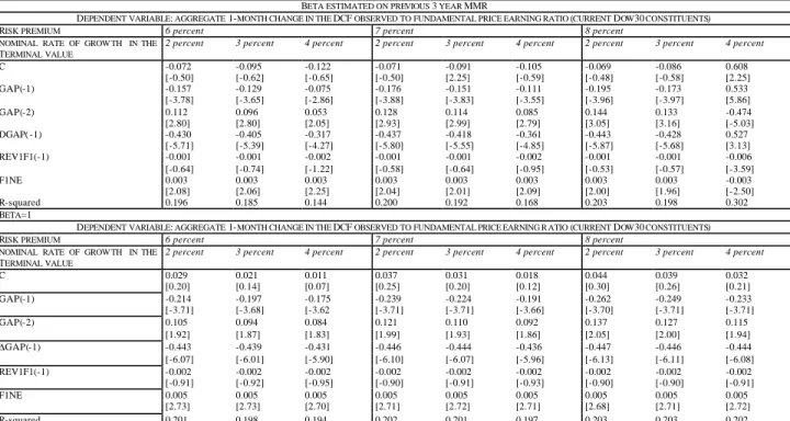
Table 2. The determinants of the aggregate DCF observed to fundamental price earning ratio (current Dow30 constituents)

BETA ESTIMATED ON PREVIOUS 3 YEAR MMR

DEPENDENT VARIABLE: AGGREGATE 1-MONTH CHANGE IN THE DCF OBSERVED TO FUNDAMENTAL PRICE EARNING RATIO (CURRENT DOW30 CONSTITUENTS)

RISK PREMIUM 6 percent 7 percent 8 percent

NOMINAL RATE OF GROW TH IN THE

TERMINAL VALUE

2 percent 3 percent 4 percent 2 percent 3 percent 4 percent 2 percent 3 percent 4 percent

C -0.072 -0.095 -0.122 -0.071 -0.091 -0.105 -0.069 -0.086 0.608 [-0.50] [-0.62] [-0.65] [-0.50] [2.25] [-0.59] [-0.48] [-0.58] [2.25] GAP(-1) -0.157 -0.129 -0.075 -0.176 -0.151 -0.111 -0.195 -0.173 0.533 [-3.78] [-3.65] [-2.86] [-3.88] [-3.83] [-3.55] [-3.96] [-3.97] [5.86] GAP(-2) 0.112 0.096 0.053 0.128 0.114 0.085 0.144 0.133 -0.474 [2.80] [2.80] [2.05] [2.93] [2.99] [2.79] [3.05] [3.16] [-5.03] DGAP( -1) -0.430 -0.405 -0.317 -0.437 -0.418 -0.361 -0.443 -0.428 0.527 [-5.71] [-5.39] [-4.27] [-5.80] [-5.55] [-4.85] [-5.87] [-5.68] [3.13] REV1F1(-1) -0.001 -0.001 -0.002 -0.001 -0.001 -0.002 -0.001 -0.001 -0.006 [-0.64] [-0.74] [-1.22] [-0.58] [-0.64] [-0.95] [-0.53] [-0.57] [-3.59] F1NE 0.003 0.003 0.003 0.003 0.003 0.003 0.003 0.003 -0.003 [2.08] [2.06] [2.25] [2.04] [2.01] [2.09] [2.00] [1.96] [-2.50] R-squared 0.196 0.185 0.144 0.200 0.192 0.168 0.203 0.198 0.302 BETA=1

DEPENDENT VARIABLE: AGGREGATE 1-MONTH CHANGE IN THE DCF OBSERVED TO FUNDAMENTAL PRICE EARNING R ATIO (CURRENT DOW30 CONSTITUENTS)

NOMINAL RATE OF GROW TH IN THE

TERMINAL VALUE

2 percent 3 percent 4 percent 2 percent 3 percent 4 percent 2 percent 3 percent 4 percent

C 0.029 0.021 0.011 0.037 0.031 0.018 0.044 0.039 0.032 [0.20] [0.14] [0.07] [0.25] [0.20] [0.12] [0.30] [0.26] [0.21] GAP(-1) -0.214 -0.197 -0.175 -0.239 -0.224 -0.191 -0.262 -0.249 -0.233 [-3.71] [-3.68] [-3.62 [-3.71] [-3.71] [-3.66] [-3.70] [-3.71] [-3.71] GAP(-2) 0.105 0.094 0.084 0.121 0.110 0.092 0.137 0.127 0.115 [1.92] [1.87] [1.83] [1.99] [1.93] [1.86] [2.05] [2.00] [1.94] ∆GAP(-1) -0.443 -0.439 -0.431 -0.446 -0.444 -0.436 -0.447 -0.446 -0.444 [-6.07] [-6.01] [-5.90] [-6.10] [-6.07] [-5.96] [-6.13] [-6.11] [-6.08] REV1F1(-1) -0.002 -0.002 -0.002 -0.002 -0.002 -0.002 -0.002 -0.002 -0.002 [-0.91] [-0.92] [-0.95] [-0.90] [-0.91] [-0.93] [-0.90] [-0.90] [-0.91] F1NE 0.005 0.005 0.005 0.005 0.005 0.005 0.005 0.005 0.005 [2.73] [2.73] [2.70] [2.71] [2.72] [2.71] [2.68] [2.71] [2.72] R-squared 0.201 0.198 0.194 0.202 0.201 0.197 0.203 0.203 0.202

T-stats are reported in square brackets. Variable legend. Dependent variable . GAP:(E/P)* - (E/P) or fundamental earning price ratio to observed earning price ratio. Regressors. ∆GAP: first difference of

the GAP variable; REV1F1=Et+1[F1]-Et[F1] where F1 is the 1-year ahead mean estimate of earning growth; F1NE: number of estimates for the 1-year ahead mean earning growth; F1SD: standard

deviation of estimates for the 1-year ahead mean earning growth.

(15)

Table 3 The effect of the aggregate DCF observed to fundamental price earning ratio (current Dow30 constituents) on Dow 30 returns

BETA ESTIMATED ON PREVIOUS 3 YEAR MMR DEPENDENT VARIABLE:1-MONTH DOW30 RETURN

NOMINAL RATE OF GROW TH IN THE TERMINAL VALUE

2 percent 3 percent 4 percent 2 percent 3 percent 4 percent 2 percent 3 percent 4 percent

C 0.017 0.017 0.018 0.017 0.017 0.018 0.017 0.017 0.021 [0.42] [0.42] [0.43] [0.41] [0.41] [0.42] [0.40] [0.41] [0.50] GAP(-1) -0.030 -0.024 -0.012 -0.033 -0.027 -0.017 -0.036 -0.030 0.050 [-2.53] [-2.41] [-1.71] [-2.56] [-2.46] [-2.05] [-2.60] [-2.50] [2.13] GAP(-2) 0.035 0.026 0.012 0.040 0.031 0.019 0.044 0.036 -0.047 [3.14] [2.84] [1.88] [3.26] [3.01] [2.40] [3.35] [3.14] [-1.96] ∆GAP(-1) -0.033 -0.030 -0.019 -0.032 -0.030 -0.021 -0.032 -0.030 0.130 [-1.77] [-1.65] [-1.16] [-1.76] [-1.65] [-1.26] [-1.75] [-1.64] [3.03] F1NE 0.0004 0.0005 0.0006 0.0003 0.0004 0.0005 0.0003 0.0003 0.0004 [0.59] [0.81] [1.15] [0.50] [0.67] [0.93] [0.44] [0.56] [0.81] F1SD -0.126 -0.125 -0.129 -0.128 -0.124 -0.123 -0.130 -0.125 -0.127 [-0.86] [-0.84] [-0.85] [-0.88] [-0.85] [-0.82] [-0.90] [-0.85] [-0.87] STLGRT 0.039 0.037 0.029 0.039 0.037 0.031 0.040 0.038 0.019 [1.66] [1.56] [1.23] [1.68] [1.59] [1.34] [1.71] [1.61] [0.87] R-squared 0.053 0.045 0.024 0.056 0.049 0.033 0.059 0.052 0.073

NOMINAL RATE OF GROW TH IN THE TERMINAL VALUE

C 0.017 0.017 0.018 0.017 0.017 0.017 0.016 0.017 0.017 [0.42] [0.43] [0.43] [0.42] [0.42] [0.43] [0.42] [0.42] [0.42] GAP(-1) -0.046 -0.042 -0.037 -0.053 -0.049 -0.041 -0.061 -0.056 -0.051 [-2.81] [-2.74] [-2.67] [-2.91] [-2.83] [-2.72] [-3.00] [-2.93] [-2.85] GAP(-2) 0.053 0.047 0.040 0.062 0.056 0.045 0.070 0.065 0.059 [3.43] [3.30] [3.14] [3.55] [3.45] [3.24] [3.65] [3.57] [3.47] ∆GAP(-1) -0.040 -0.039 -0.039 -0.040 -0.040 -0.039 -0.041 -0.040 -0.040 [-2.10] [-2.09] [-2.07] [-2.13] [-2.11] [-2.09] [-2.15] [-2.13] [-2.11] F1NE 0.0003 0.0004 0.0004 0.0003 0.0003 0.0004 0.0003 0.0003 0.0003 [0.52] [0.57] [0.66] [0.51] [0.52] [0.61] [0.51] [0.51] [0.52] F1SD -0.126 -0.121 -0.116 -0.130 -0.126 -0.119 -0.134 -0.131 -0.127 [-0.86] [-0.83] [-0.80] [-0.89] [-0.87] [-0.82] [-0.92] [-0.90] [-0.87] STLGRT 0.040 0.039 0.038 0.041 0.040 0.039 0.042 0.041 0.041 [1.77] [1.73] [1.68] [1.82] [1.78] [1.71] [1.85] [1.82] [1.79] R-squared 0.065 0.062 0.058 0.068 0.065 0.060 0.071 0.068 0.066

T-stats are reported in square brackets. Variable legend. GAP:(E/P)* - (E/P) or fundamental earning price ratio to observed earning price ratio (current Dow30 constituents).

Regressors.

∆GAP: first difference of the GAP variable; F1NE: number of estimates for the 1-year ahead mean earning growth; F1NE: number of estimates for the 1-year ahead mean earning growth; F1SD: standard deviation of estimates for the 1-year ahead mean earning growth; STLGRT: mean 1-year ahead to mean long term forecasted

(16)

Table 4. Relative performance of value and growth DCF strategies on Dow stocks GROWTH PORTFOLI O AVERAGE PORTFOLI O VALUE PORTFOLI O BUY AND HOLD ON DOW30 BUY AND HOLD ON DOW65 GROWTH PORTFOLI O AVERAGE PORTFOLI O VALUE PORTFOLI O BUY AND HOLD ON DOW30 BUY AND HOLD ON DOW65

MEAN MONTHLY RETURNS MEAN MONTHLY RETURNS

RISK PREMIUM 6PERCENT, NOMINAL GROWTH IN THE TERMINAL PERIOD 3PERCENT, VARIABLE BETA

RISK PREMIUM 8PERCENT, NOMINAL GROWTH IN THE TERMINAL PERIOD 3PERCENT, UNIT BETA

1 month 2.580 1.300 0.850 1.600 1.040 2.611 1.389 0.796 1.600 1.040 Lagged 1 month 2.697 1.498 0.667 2.910 1.383 0.620 2 months 2.630 1.390 0.760 2.669 1.466 0.670 6 months 2.050 1.440 1.270 2.057 1.360 1.320 12 months 1.905 1.470 1.340 1.847 1.389 1.534

MONTHLY RETURNS VARIANCE MONTHLY RETURNS VARIANCE

1 month 0.0026 0.0024 0.0025 0.0024 0.0022 0.0031 Lagged 1 month 0.0026 0.0025 0.0024 0.0024 0.0022 0.0032 2 months 0.0026 0.0024 0.0024 0.0024 0.0023 0.0031 6 months 0.0028 0.0026 0.0022 0.0026 0.0021 0.0031 12 months 0.0029 0.0022 0.0024 0.0022 0.0017 0.0026 0.0022 0.0029 0.0022 0.0017

MONTHLY RETURNS SKEWNESS MONTHLY RETURNS SKEWNESS

1 month -0.377 -0.655 -0.582 -0.272 -0.542 -0.565 Lagged 1 month -0.455 -0.579 -0.477 -0.279 -0.576 -0.504 2 months -0.377 -0.568 -0.675 -0.198 -0.562 -0.572 6 months -0.440 -0.820 -0.089 -0.241 -0.489 -0.357 12 months -0.609 -0.557 -0.197 -0.560 -0.774 -0.334 -0.394 -0.446 -0.560 -0.774

Legend for all strategies except lagged 1 month: portfolios are formed the first day of month t on values that the ranking variable (value to price ratio) assumes in the last day of the month t-1 and held until the end of month t (1 month strategy), t+1 (two month strategy), t+6 (6 month strategy). New portfolios are formed only at the end of each holding period. Lagged 1 month: portfolios are formed the first day of month t+1 on values that the ranking variable (value to price ratio) assumes in the last day of the month t-1 and held until the end of month t+1.

(17)

Table 5a. Significance of the difference in unc onditional mean monthly returns of different portfolio strategies

RISK PREMIUM 6PERCENT, NOMINAL GROWTH IN THE TERMINAL PERIOD 3PERCENT,

VARIABLE BETA

INTERVAL BETWEEN TWO SUBSEQUENT PORTFOLIO RECOMPOSITIONS IN GROWTH AND VALUE STRATEGIES

PORTFOLIO STRATEGIES T-STAT Nonparametric test

z Prob > |z| Lagged 1 month 4.319 4.556 0.00001 1 month 3.649 3.816 0.0001 2 months 4.037 4.193 0.00001 6 months 1.839 2.326 0.0200 1 year VALUE PORTFOLIOS VERSUS GROWTH PORFOLIOS 1.234 1.561 0.1184

Lagged 1 month DJ65 VERSUS GROWTH -3.774 -4.013 0.0000 DJ65 VERSUS VALUE 0.889 1.087 0.2769

1 month DJ65 VERSUS GROWTH -3.529 -3.758 0.0002 DJ65 VERSUS VALUE 0.447 0.463 0.6436

2 months DJ65 VERSUS GROWTH -3.518 -3.782 0.0002 DJ65 VERSUS VALUE 0.848 0.845 0.3981

6 months DJ65 VERSUS GROWTH -2.324 -2.738 0.0062 DJ65 VERSUS VALUE -0.412 0.157 0.8752

1 year DJ65 VERSUS GROWTH -2.002 -2.325 0.0201 DJ65 VERSUS VALUE -0.720 0.671 0.5023

1 year DJ30 VERSUS GROWTH -0.733 -0.934 0.3504 DJ30 VERSUS VALUE 0.553 0.702 0.4826 For the definition of portfolio strategies see legend at Table 4

The non parametric test is based on the Mann-Withney U-statistics computed as

follows: ₁ ₂ 1 1 ₁

2 )

1 (

R

N

U

=

+

−

and ₁ ₂ 2 2 ₂

2 )

1 (

R

N

U

=

+

−

where

N

₁ is the number of observations in the first sample,

N

₂ is the number of observations in the second

sample,

R

₁ is the sum of ranks in the first sample,

R

₂ is the sum of ranks in the second sample. The test

(18)

Table 5b Significance of the difference in unconditional mean monthly returns of different portfolio strategies

RISK PREMIUM 8 PERCENT, NOMINAL GROWTH IN THE TERMINAL PERIOD 3PERCENT,

BETA=1

INTERVAL BETWEEN TWO SUBSEQUENT PORTFOLIO RECOMPOSITIONS IN GROWTH AND VALUE STRATEGIES

PORTFOLIO STRATEGIES T-STAT Nonparametric test

z Prob > |z| Lagged 1 month 4.630 4.778 0.00001 1 month 3.692 3.664 0.0002 2 months 4.083 4.068 0.0002 6 months 1.469 1.795 0.0727 1 year VALUE PORTFOLIOS VERSUS GROWTH PORFOLIOS 0.638 0.837 0.4026

6 months DJ65 VERSUS GROWTH 2.570 2.570 0.0100 DJ65 VERSUS VALUE -0.591 0.490 0.6240

1 year DJ65 VERSUS GROWTH -1.842 -2.048 0.0400 DJ65 VERSUS VALUE -1.073 -1.055 0.2900

1 year DJ30 VERSUS GROWTH -0.536 -0.626 0.5310 DJ30 VERSUS VALUE 0.145 0.338 0.7357 For the definition of portfolio strategies see legend at Table 4

The non parametric test is based on the Mann-Withney U-statistics computed as

follows: ₁ ₂ 1 1 ₁

2 )

1 (

R

N

U

=

+

−

and ₁ ₂ 2 2 ₂

2 )

1 (

R

N

U

=

+

−

where

N

1 is the

number of observations in the first sample,

N

₂ is the number of observations in the second sample,

R

₁ is the sum of

(19)

Table 6 Risk adjustment of returns from growth and value DCF strategies with CAPM (GMM estimates)

VARIABLE BETA

RM: MEAN MONTHLY RETURNS ON DATASTREAM WORLDINDEX STRATEG

Y

HOLDING PERIOD

1 MONTH 2 MONTHS 6 MONTHS 1 YEAR

STRATEG Y

GROWTH VALUE GROWTH VALUE GROWTH VALUE GROWTH VALUE

C 0.010 -0.010 0.009 -0.011 0.004 -0.006 0.002 -0.003 [3.10] [-2.29] [2.71] [-2.79] [1.13] [-1.65] [0.49] [-0.77] Rm-Rf 0.861 0.765 0.848 0.783 0.815 0.834 0.771 0.826 [7.90] [5.41] [7.20] [5.95] [7.18] [8.84] [5.94] [6.14] (Rm-Rf)2 -0.059 -0.668 -0.007 -0.509 -0.364 0.074 -0.660 -0.236 [-0.06] [-0.57] [-0.01] [-0.45] [-0.41] [0.10] [-0.57] [-0.24] Rsquared 0.553 0.527 0.526 0.544 0.521 0.552 0.505 0.565

BETA=1

RM: MEAN MONTHLY RETURNS ON DATASTREAM WORLDINDEX STRATEG

Y

HOLDING PERIOD

STRATEG Y

GROWTH VALUE GROWTH VALUE GROWTH VALUE GROWTH VALUE

C 0.008 -0.007 0.008 -0.008 0.006 -0.002 0.002 0.0001 [1.78] [-1.60] [1.88] [-1.86] [1.38] [-0.31] [0.63] [0.01] Rm-Rf 0.854 0.784 0.860 0.776 0.960 0.818 0.903 0.791 [6.06] [5.39] [5.89] [5.59] [7.07] [5.61] [6.66] [5.20] (Rm-Rf)2 0.332 -1.024 0.473 -1.140 0.760 -0.786 0.369 -0.953 [0.29] [-0.91] [0.39] [-1.07] [0.72] [-0.69] [0.33] [-0.80] Rsquared 0.522 0.517 0.511 0.530 0.556 0.513 0.561 0.526

The table reports coefficients and t-tests of the following 3-CAPM regression :

ε

γ

β

α

+

−

+

−

+

=

−

₍

₎

₍

₎

2 f m f m f PK

R

where Rpk is the monthly return of portfolio p (p=1,..,11) formed on factor k, Rf is the monthly return of the

3-month UK average deposit interest rate for the same period, Rm is the monthly return of the sample market

portfolio Equations are estimated with a GMM (Generalised Method of Moments) approach with Heteroskedasticity and Autocorrelation Consistent Covariance Matrix. The Bartlett’s functional form of the kernel is used to weight the covariances in calculating the weighting matrix. Newey and West’s (1994) automatic bandwidth procedure is adopted to determine weights inside kernels for autocovariances. The same regressors are used as instruments.

* The coefficient is significantly different from zero at 95%. ** The coefficient is significantly different from zero at 99%.

Dependent variable legend:

(20)

Table 7. Relative performance of value and growth strategies on the historical Dow30 components

GROWTH PORTFOLI O AVERAGE PORTFOLI O VALUE PORTFOLI O BUY AND HOLD ON DOW30 BUY AND HOLD ON DOW65

MEAN MONTHLY RETURNS

1 month 2.25 1.32 0.12 1 month interv. 1.36 1.16 0.40 2 months 2.13 1.25 0.36 6 months 1.84 1.24 0.78 12 months 1.85 1.13 0.92 1.600 1.040 GROWTH PORTFOLI O AVERAGE PORTFOLI O VALUE PORTFOLI O BUY AND HOLD ON DOW30 BUY AND HOLD ON DOW65

VARIANCE OF MONTHLY RETURNS

1 month 0.020 0.002 0.003 0.0022 0.0017 1 month interv. 0.002 0.002 0.003 2 months 0.020 0.002 0.003 6 months 0.020 0.002 0.003 12 months 0.020 0.002 0.003 GROWTH PORTFOLI O AVERAGE PORTFOLI O VALUE PORTFOLI O BUY AND HOLD ON DOW30 BUY AND HOLD ON DOW65

SKEWNESS OF MONTHLY RETURNS

1 month 0.165 -0.849 -1.120 1 month interv. -0.429 -0.914 -0.814 2 months -0.221 -0.922 -1.074 6 months 0.096 -0.819 -0.762 12 months 0.070 -0.816 -0.846 -0.56 -0.774

(21)

Table 8. Significance of the difference in unconditional mean monthly returns of different portfolio strategies on the historical Dow30 components

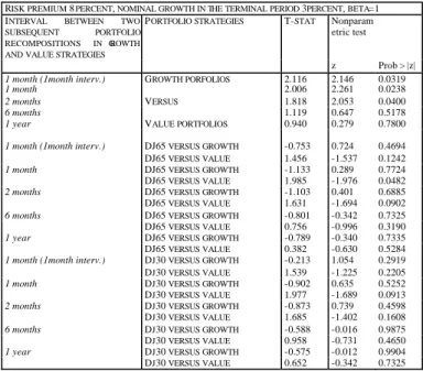
RISK PREMIUM 8 PERCENT, NOMINAL GROWTH IN THE TERMINAL PERIOD 3PERCENT, BETA=1 INTERVAL BETWEEN TWO

SUBSEQUENT PORTFOLIO RECOMPOSITIONS IN GROWTH AND VALUE STRATEGIES

PORTFOLIO STRATEGIES T-STAT Nonparam etric test

z Prob > |z|

1 month (1month interv.) 2.116 2.146 0.0319

1 month 2.006 2.261 0.0238 2 months 1.818 2.053 0.0400 6 months 1.119 0.647 0.5178 1 year GROWTH PORFOLIOS VERSUS VALUE PORTFOLIOS 0.940 0.279 0.7800

1 month (1month interv.) DJ65 VERSUS GROWTH -0.753 0.724 0.4694 DJ65 VERSUS VALUE 1.456 -1.537 0.1242

1 month DJ65 VERSUS GROWTH -1.133 0.289 0.7724 DJ65 VERSUS VALUE 1.985 -1.976 0.0482

2 months DJ65 VERSUS GROWTH -1.103 0.401 0.6885 DJ65 VERSUS VALUE 1.631 -1.694 0.0902

6 months DJ65 VERSUS GROWTH -0.801 -0.342 0.7325 DJ65 VERSUS VALUE 0.756 -0.996 0.3190

1 year DJ65 VERSUS GROWTH -0.789 -0.340 0.7335 DJ65 VERSUS VALUE 0.382 -0.630 0.5284

1 month (1month interv.) DJ30 VERSUS GROWTH -0.213 1.054 0.2919 DJ30 VERSUS VALUE 1.539 -1.225 0.2205

1 month DJ30 VERSUS GROWTH -0.902 0.635 0.5252 DJ30 VERSUS VALUE 1.977 -1.689 0.0913

2 months DJ30 VERSUS GROWTH -0.873 0.739 0.4598 DJ30 VERSUS VALUE 1.685 -1.402 0.1608

6 months DJ30 VERSUS GROWTH -0.588 -0.016 0.9875 DJ30 VERSUS VALUE 0.958 -0.731 0.4650

1 year DJ30 VERSUS GROWTH -0.575 -0.012 0.9904 DJ30 VERSUS VALUE 0.652 -0.342 0.7325

(22)

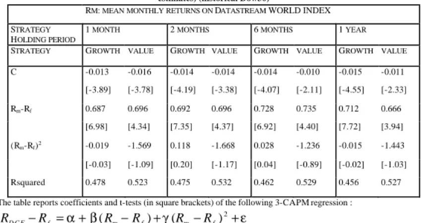
Table 9. Risk adjustment of returns from growth and value DCF strategies with CAPM (GMM estimates) (historical Dow30)

RM: MEAN MONTHLY RETURNS ON DATASTREAM WORLDINDEX STRATEGY

HOLDING PERIOD

STRATEGY GROWTH VALUE GROWTH VALUE GROWTH VALUE GROWTH VALUE

C -0.013 -0.016 -0.014 -0.014 -0.014 -0.010 -0.015 -0.011 [-3.89] [-3.78] [-4.19] [-3.38] [-4.07] [-2.11] [-4.55] [-2.33] Rm-Rf 0.687 0.696 0.692 0.696 0.728 0.735 0.712 0.666 [6.98] [4.34] [7.35] [4.37] [6.92] [4.40] [7.72] [3.94] (Rm-Rf)2 -0.019 -1.569 0.118 -1.668 0.028 -1.236 -0.015 -1.443 [-0.03] [-1.09] [0.20] [-1.17] [0.04] [-0.89] [-0.02] [-1.03] Rsquared 0.478 0.523 0.475 0.532 0.462 0.529 0.456 0.527

The table reports coefficients and t-tests (in square brackets) of the following 3-CAPM regression :

ε

γ

β

α

+

−

+

−

+

=

−

2

)

(

)

(

m f m f f D C F

R

where RDCF is the monthly return of the DCF portfolio, Rf is the monthly return of the 3-month US T-bill for the same

period, Rm is the monthly return of the sample market portfolio Equations are estimated with a GMM (Generalised

Method of Moments) approach with Heteroskedasticity and Autocorrelation Consistent Covariance Matrix. The Bartlett’s functional form of the kernel is used to weight the covariances in calculating the weighting matrix. Newey and West’s (1994) automatic bandwidth procedure is adopted to determine weights inside kernels for autocovariances. The same regressors are used as instruments.

(23)

Table 10. The determinants of the aggregate DCF observed to fundamental price earning ratio (historical Dow30 constituents)

BETA ESTIMATED ON PREVIOUS 3 YEAR MMR

DEPENDENT VARIABLE: AGGREGATE 1-MONTH CHANGE IN THE DCF OBSERVED TO FUNDAMENTAL EARNING TO PRIC E RATIO

(HISTORICAL DOW30 CONSTITUENTS)

NOMINAL RATE OF GROWTH IN THE

TERMINAL VALUE

C -0.072 -0.095 -0.122 -0.071 -0.091 -0.105 -0.069 -0.086 0.608 [-0.50] [-0.62] [-0.65] [-0.50] [2.25] [-0.59] [-0.48] [-0.58] [2.25] GAP(-1) -0.019 0.015 -0.033 0.013 -0.082 0.006 -0.792 -0.025 -0.082 [-0.70] [0.18] [-0.50] [0.26] [-0.65] [0.02] [-2.17] [-0.27] [-0.81] GAP(-2) -0.048 0.019 0.021 -0.176 -0.042 -0.042 -0.528 0.001 0.063 [-1.82] [0.23] [0.33] [-3.57] [-0.33] [-0.19] [-1.43] [0.01] [0.62] ∆GAP(-1) -0.112 -0.029 -0.016 0.226 -0.068 -0.016 0.010 -0.003 -0.033 [-1.68] [-0.43] [-0.24] [3.52] [-1.01] [-0.24] [0.15] [-0.04] [-0.49] REV1F1(-1) -0.0001 -0.0007 -0.0045 0.0001 -0.0010 -0.0050 0.0009 0.0008 -0.0005 [-0.07] [-0.12] [-0.26] [0.07] [-0.12] [-0.21] [0.06] [0.07] [-0.08] F1NE 0.005 0.006 0.008 0.007 0.022 0.020 0.052 0.004 0.007 [1.98] [0.62] [0.35] [2.28] [1.57] [0.57] [1.62] [0.23] [0.62] R-squared 0.029 0.001 0.002 0.114 0.006 0.000 0.032 0.0003 0.006 BETA=1

DEPENDENT VARIABLE: AGGREGATE 1-MONTH CHANGE IN THE DCF OBSERVED TO FUNDAMENTAL EARNING TO PRIC E RATIO

(HISTORICAL DOW30 CONSTITUENTS)

TERMINAL VALUE

2 percent 3 percent 4 percent 2 perc ent 3 percent 4 percent 2 percent 3 percent 4 percent

C 0.029 0.021 0.011 0.037 0.031 0.018 0.044 0.039 0.032 [0.20] [0.14] [0.07] [0.25] [0.20] [0.12] [0.30] [0.26] [0.21] GAP(-1) -0.205 -0.189 -0.169 -0.228 -0.214 -0.198 -0.249 -0.237 -0.223 [-3.42] [-3.40] [-3.34] [-3.41] [-3.42] [-3.40] [-3.38] [-3.40] [-3.41] GAP(-2) 0.075 0.066 0.057 0.088 0.079 0.069 0.102 0.093 0.083 [1.31] [1.25] [1.20] [1.39] [1.33] [1.26] [1.46] [1.40] [1.34] ∆GAP(-1) -0.444 -0.441 -0.435 -0.446 -0.445 -0.442 -0.447 -0.447 -0.445 [-6.79] [-6.74] [-6.64] [-6.82] [-6.79] [-6.75] [-6.83] [-6.84] [-6.80] REV1F1(-1) -0.0001 -0.0001 -0.0001 -0.0001 -0.0001 -0.0001 -0.0001 -0.0001 -0.0001 [-0.43] [-0.43] [-0.43] [-0.43] [-0.43] [-0.43] [-0.43] [-0.43] [-0.43] F1NE 0.006 0.006 0.006 0.006 0.006 0.006 0.006 0.006 0.006 [3.06] [3.06] [3.01] [3.05] [3.06] [3.06] [3.03] [3.05] [3.06] R-squared 0.180 0.177 0.173 0.181 0.180 0.178 0.181 0.182 0.180

T-stats are reported in square brackets. Variable legend. Dependent variable . GAP = (E/P)* - (E/P) or fundamental earning price

ratio to observed earning price ratio. Regressors. ∆GAP: first difference of the GAP variable; REV1F1=Et+1[F1]-Et[F1] where

(24)

Table 11. The effect of the aggregate DCF observed to fundamental price earning ratio (historical Dow30 constituents) on Dow 30 returns

TERMINAL VALUE

C 0.017 0.017 0.018 0.017 0.017 0.018 0.017 0.017 0.021 [0.42] [0.42] [0.43] [0.41] [0.41] [0.42] [0.40] [0.41] [0.50] GAP(-1) 0.002 0.001 0.0005 0.003 0.002 0.0003 0.001 -0.0005 -0.002 [0.77] [0.81] [1.37] [0.80] [1.10] [0.34] [0.38] [-0.63] [-1.48] GAP(-2) 0.000 0.001 0.0002 0.001 0.001 0.00002 -0.0003 0.0004 0.001 [-0.17] [0.49] [0.55] [0.13] [0.62] [0.003] [-0.13] [0.61] [0.34] ∆GAP(-1) -0.008 0.003 -0.0001 -0.008 -0.0002 0.0001 0.0001 0.001 0.002 [-1.29] [2.34] [-0.19] [-1.46] [-0.27] [0.38] [0.29] [1.50] [1.94] F1NE 0.0002 0.0001 0.0002 0.0001 0.0001 0.0003 0.0002 0.0003 0.0004 [0.82] [0.86] [1.62] [0.21] [0.78] [1.72] [1.22] [1.90] [1.96] F1SD 0.003 0.003 0.003 0.003 0.003 0.003 0.003 0.003 0.003 [0.94] [1.02] [0.99] [0.93] [0.92] [0.98] [0.97] [1.00] [1.06] STLGRT 0.0002 0.0002 0.0002 0.0002 0.0002 0.0002 0.0002 0.0002 0.0002 [1.03] [1.01] [1.14] [1.01] [0.96] [1.00] [0.96] [1.00] [1.02] R-squared 0.017 0.034 0.018 0.019 0.015 0.008 0.008 0.020 0.034

TERMINAL VALUE

C 0.017 0.017 0.018 0.017 0.017 0.017 0.016 0.017 0.017 [0.42] [0.43] [0.43] [0.42] [0.42] [0.43] [0.42] [0.42] [0.42] GAP(-1) -0.030 -0.027 -0.023 -0.035 -0.031 -0.028 -0.040 -0.037 -0.033 [-1.77] [-1.74] [-1.72] [-1.83] [-1.79] [-1.75] [-1.90] [-1.87] [-1.80] GAP(-2) 0.041 0.036 0.031 0.048 0.044 0.038 0.055 0.051 0.046 [2.59] [2.50] [2.37] [2.68] [2.61] [2.51] [2.75] [2.70] [2.62] ∆GAP(-1) -0.042 -0.042 -0.041 -0.043 -0.042 -0.042 -0.043 -0.042 -0.043 [-2.34] [-2.33] [-2.34] [-2.36] [-2.35] [-2.34] [-2.39] [-2.34] [-2.35] F1NE -0.0002 -0.0001 -0.0001 -0.0002 -0.0002 -0.0001 -0.0002 -0.0002 -0.0002 [-0.28] [-0.21] [-0.10] [-0.31] [-0.28] [-0.22] [-0.32] [-0.30] [-0.28] F1SD 0.001 0.001 0.002 0.0004 0.001 0.001 0.0002 0.0005 0.001 [0.17] [0.28] [0.43] [0.10] [0.17] [0.27] [0.05] [0.10] [0.16] STLGRT 0.0003 0.0003 0.0003 0.0003 0.0003 0.0003 0.0003 0.0003 0.0003 [1.68] [1.66] [1.63] [1.71] [1.69] [1.66] [1.74] [1.71] [1.69] R-squared 0.053 0.051 0.049 0.055 0.054 0.052 0.057 0.055 0.054

T-stats are reported in square brackets. Variable legend. GAP = (E/P)* - (E/P) or fundamental earning price ratio to observed

earning price ratio. (current Dow30 constituents); Regressors. ∆GAP: first difference of the GAP variable REV1F1=Et+1

[F1]-Et[F1] where F1 is the 1-year ahead mean estimate of earning growth; REV2F1: Et+2[F1]-Et+1[F1]; F1NE: number of estimates

for the 1-year ahead mean earning growth; F1NE: number of estimates for the 1-year ahead mean earning growth; F1SD: standard deviation of estimates for the 1-year ahead mean earning growth; STLGRT: mean 1-year ahead to mean long te rm forecasted earning growth.

(25)

References

Ball, R. and Kothari, S. P., 1998, Nonstationary Expected

Returns: Implications for Tests of Market Efficiency and Serial

Correlation in Returns; Journal of Financial Economics, 25, (1),

pp. 51-74

Black. F., 1972, Capital Market Equilibrium with restricted

borrowing, Journal of Business, 45,

Brennan, M. J. Jegadeesh, N.; Swaminathan, B. (1993);

“Investment Analysis and the Adjustment of Stock Prices to

Common Information” Review of Financial Studies; 6(4),

pp.799-824

Campbell, J.Y., 2000, Asset pricing at the Millennium, Journal of

Finance, 55 (4), pp. 1515-1567.

De Long, J.B., A. Shleifer, L. Summers and R.J. Waldmann,

1990, 'Noise Trader Risk in Financial Markets', Journal of

Political Economy, 98 (4) , pp.701-738.

Fama, E.F. and K.R. French, 1992, The Cross-section of expected

stock returns, Journal of Finance, 47 (2), pp. 427-465.

Fama, E.F. and K.R. French, 1993, Common risk factors in the

returns on stock and bonds, Journal of Financial Economics, 33

(1), pp. 3-56.

Fama, E.F. and K.R. French, 1996, Multifactor explanations of

asset pricing anomalies, Journal of Finance, 51 (1), pp. 55-84.

Fama, E.F. and K.R. French, 1998, Value versus growth: the

international evidence, Journal of Finance, 53, ( 6), pp. 1975-99

Farrelly , G.E. Reichenstein, W.R., 1984, Risk perception of

institutional investors, Journal of Portfolio Management, Vol. 10,

pp. 5-12.

Firth, Michael; Gift, Michael (1999) “An International

Comparison of Analysts' Earnings Forecast Accuracy”

International Advances in Economic Research; 5(1), pp. 56-64.

Frankel, R. and Lee, C. M. C., Accounting Valuation, Market

Expectation, and Cross-Sectional Stock Returns, Journal of

Accounting and Economics; 25(3), June 1998, pp. 283-319.

(26)

Gordon M. and Shapiro E. (1956) "Capital Equipment Analysis,

the Required Rate of Profit" Management Science, pp.102-110.

Harvey, C. R. and Siddique, A., 2000, Conditional Skewness in

Asset Pricing Tests; Journal of Finance, 55, (3), pp. 1263-95

Jagannathan, R. and Wang Z., 1996 , The conditional CAPM and

the cross-section of expected returns, The Journal of Finance

51(1), pp.3-53.

Jeegadesh, N. Titman S., 1993, Returns to buying winners and

selling losers: implications for stock market efficiency, Journal of

Finance, 48 (1), pp. 65-91.

Kaplan S.N., Roeback, R.S., 1995, The valuation of cash flow

forecasts: an empirical analysis, Journal of Finance, 50 (4), pp.

1059-1093.

Lakonishok, J., Shleifer, A. and R.W. Vishny, 1994, Contrarian

investment, extrapolation and risk, Journal of Finance, 49, pp.

1541-1578.

Lamont, O., 1998, Earnings and expected returns, Journal of

Finance, 53 (5), pp.1563-1587.

Lee, C. M. C.; Myers,J. and Swaminathan, B., 1999, What Is the

Intrinsic Value of the Dow?, Journal of Finance; 54(5), pp.

1693-1741.

Linter, J., 1965, The valuation of risk assets and the selection of

risky investments in stock portfolios and capital budgets, Review

of Economics and Statistics, 47, pp.13-37.

Lo, A., MacKinlay, 1990, When are contrarian profits due to

stock market overreaction ?, Review of Financial Studies, 3 (2),

pp.175-208.

Miller M. H. and Modigliani F., 1961, Dividend Policy, Growth

and the Valuation of Shares Journal of Business, pp.411-33.

Newey, W. K. and West, Kenneth D., 1994,Automatic Lag

Selection in Covariance Matrix Estimation; Review of Economic

Studies, October, 61, (4), pp. 631-53

Ohlson J. A., 1995, Earnings, Book Value, and Dividends in

Equity Valuation, Contemporary Accounting Research, pp.

661-87.

(27)

Parkash, M., Salakta W.K., 1999, The relation of analysts'

forecast dispersion with business risk, and information

availability, mimeo.

Rouwenhorst, K.G., 1998, International momentum strategies,

Journal of Finance, 53, pp.267-285.

Sharpe, W.F., 1964, Capital asset prices: a theory of market

equilibrium under conditions of risk, Journal of Finance, 19, pp.

425-442.

Wang, Y. 1993, Near Rational Behaviour and Financial Market

Fluctuations, The Economic Journal, 103 (421), pp. 1462-1478.

(28)

Appendix (not to be published and available upon request)

Table A.1 Relative performance of non overlapping value and growth DCF strategies on Dow stocks in sample subperiods (1982-1991; 1992-2000)

RISK PREMIUM 6PERCENT, NOMINAL GROWTH IN THE TERMINAL PERIOD 3PERCENT, VARIABLE BETA LAGGED 1 MONTH LAGGED 1 MONTH

1 month MI 2.623 2.888 mI 0.710 0.603 MII 2.495 2.506 mII 0.998 0.732 varI 0.003 0.003 varI 0.003 0.003 varII 0.002 0.002 varII 0.002 0.002 2 months mI 2.755 mI 0.566 mII 2.414 mII 0.803 varI 0.003 varI 0.003 varII 0.002 varII 0.002 6 months mI 2.219 mI 1.074 mII 1.941 mII 1.365 varI 0.003 varI 0.002 varII 0.002 varII 0.002 1 year mI 2.161 mI 1.192 mII 1.734 mII 1.518 varI 0.004 varI 0.003 G R O W H T P O R T F O L I O S varII 0.002 V A L U E P O R T F O L I O S varII 0.002 mI 1.095 mII 1.000 varI 0.002 DOW JONES 65 varII 0.001 DOW JONES 30 mI 0.017 mII 0.016 varI 0.003 varII 0.002

Legend: m1 mean monthly return from the corresponding portfolio strategy for the period 1982-1991; mII mean monthly return from the corresponding portfolio strategy for the period 1992-2000; var1 variance of

monthly returns from thecorresponding portfolio strategy for the period 1982-1991; varII variance of

monthly returns from the corresponding portfolio strategy for the period 1992-2000; For portfolio strategies see legend at Table 4

(29)

Table A.2 Relative performance of non overlapping value and growth DCF strategies on Dow stocks in sample subperiods (1982-1991; 1992-2000)

RISK PREMIUM 8 PERCENT, NOMINAL GROWTH IN THE TERMINAL PERIOD 3PERCENT, BETA=1

LAGGED 1 MONTH LAGGED 1 MONTH

1 month mI 2.793 3.154 mI 0.640 0.365 mII 2.428 2.665 mII 0.952 0.875 varI 0.308 0.321 varI 0.346 0.338 varII 0.176 0.162 varII 0.276 0.297 2 months mI 2.939 mI 0.532 mII 2.399 mII 0.808 varI 0.313 varI 0.327 varII 0.170 varII 0.286 6 months mI 2.388 mI 1.035 mII 1.725 mII 1.605 varI 0.298 varI 0.322 varII 0.228 varII 0.300 1 year mI 2.260 mI 1.114 mII 1.434 mII 1.954 varI 0.311 varI 0.314 G R O W H T P O R T F O L I O S varII 0.199 V A L U E P O R T F O L I O S varII 0.274 mI 1.095 mll 1.000 varl 0.220 DOW JONES 65 varll 0.130 DOW JONES 30 mI 1.655 mII 1.551 varI 0.281 varII 0.158

Legend: m1 mean monthly return from the corresponding portfolio str ategy for the period 1982-1991; mII mean monthly return from the corresponding portfolio strategy for the period 1992-2000; var1 variance of monthly returns from the corresponding portfolio strategy for the period 1982-1991; varII variance of monthly returns from the corresponding portfolio strategy for the period 1992-2000;

(30)

Table A.3 Significance of the difference in unconditional mean monthly returns of different portfolio strategies in sample subperiods

VARIABLE BETA LAGGED 1 MONTH LAGGED 1 MONTH 1month-I subperiod 3.705 4.408 1month-II subperiod 3.496 4.247 2month-I subperiod 4.261 2month-II subperiod 3.792 6month-I subperiod 2.281 6month-II subperiod 1.330 1year-I subperiod 1.853 GROWTH VERSUS VALUE 1year-II subperiod 0.497 1month-I subperiod -3.134 -3.654 1month-I subperiod 0.817 1.047 1month-II subperiod -3.973 -3.989 1month-II subperiod 0.006 0.701 2month-I subperiod -3.395 2month-I subperiod 1.133 2month-II subperiod -3.724 2month-II subperiod 0.508 6month-I subperiod -2.283 6month-I subperiod 0.046 6month-II subperiod -2.399 6month-II subperiod - 0.952 1year-I subperiod -2.123 1year-I subperiod - 0.208 DOW JONES 65 VERSUS VALUE PORTFOLI OS 1year-II subperiod -1.874 DOW JONES 65 VERSUS VALUE PORTFOLI OS 1year-II subperiod - 1.338 1month-I subperiod -1.884 -2.386 1month-I subperiod 1.894 2.113 1month-II subperiod -2.407 -2.427 1month-II subperiod 1.351 2.060 2month-I subperiod -2.136 2month-I subperiod 2.201 2month-II subperiod -2.181 2month-II subperiod 1.856 6month-I subperiod -1.089 6month-I subperiod 1.212 6month-II subperiod -0.957 6month-II subperiod 0.465 1year-I subperiod -0.959 1year-I subperiod 0.942 DOW JONES 30 VERSUS VALUE PORTFOLI OS 1year-II subperiod -0.450 DOW JONES 30 VERSUS VALUE PORTFOLI OS 1year-II subperiod 0.083 For portfolio strategies see legend at Table 4

(31)

Table A.4 Significance of the difference in unconditional mean monthly returns of different portfolio strategies in sample subperiods

BETA=1 LAGGED 1 MONTH LAGGED 1 MONTH 1month-I subperiod 4.754 5.189 1month-II subperiod 3.313 3.991 2month-I subperiod 6.087 2m onth-II subperiod 3.552 6month-I subperiod 2.826 6month-II subperiod 0.250 1year-I subperiod 2.395 GROWTH VERSUS VALUE 1year-II subperiod -1.140 1month-I subperiod -3.973 -4.226 1month-I subperiod 0.980 1.476 1month-II subperiod -3.887 -4.658 1month-II subperiod 0.113 0.289 2month-I subperiod -4.148 2month-I subperiod 1.443 2month-II subperiod -3.850 2month-II subperiod 0.449 6month-I subperiod -3.009 6month-I subperiod 0.123 6month-II subperiod -1.825 6month-II subperiod -1.393 1year-I subperiod -2.713 1year-I subperiod -0.038 DOW JONES 65 VERSUS GROWTH PORTFOLI OS 1year-II subperiod -1.140 DOW JONES 65 VERSUS VALUE PORTFOLI OS 1year-II subperiod -2.267 1month-I subperiod -2.490 -2.919 1month-I subperiod 2.062 2.476 1month-II subperiod -2.285 -2.977 1month-II subperiod 1.376 1.514 2month-I subperiod -2.713 2month-I subperiod 2.656 2month-II subperiod -2.232 2month-II subperiod 1.684 6month-I subperiod -1.596 6month-I subperiod 1.205 6month-II subperiod -0.422 6month-II subperiod -0.120 1year-I subperiod -1.319 1year-I subperiod 1.052 DOW JONES 30 VERSUS GROWTH PORTFOLI OS 1year-II subperiod 0.295 DOW JONES 30 VERSUS VALUE PORTFOLI OS 1year-II subperiod -0.926 For portf olio strategies see legend at Table 4

(32)

Table A.5 Relative performance of non overlapping value and growth sophisticated DCF strategies on hystorical Dow30 components in sample subperiods (1982-1991; 1992-2000)

RISK PREMIUM 8 PERCENT, NOMINAL GROWTH IN THE TERMINAL PERIOD 3PERCENT, BETA=1

1 month mI 0.030 0.012 mI 0.001 0.004 mII 0.014 0.015 mII 0.002 0.003 VarI 0.038596 0.00181 varI 0.003635 0.003636 VarII 0.001487 0.001349 varII 0.002521 0.002599 2 months MI 0.030 mI 0.004 MII 0.013 mII 0.002 VarI 0.038522 varI 0.003711 varII 0.001474 varII 0.002553 6 months mI 0.028 mI 0.007 mII 0.009 mII 0.007 varI 0.038601 varI 0.003535 varII 0.002302 varII 0.002522 1 year mI 0.028 mI 0.008 mII 0.009 mII 0.009 varI 0.038647 varI 0.003185 G R O W H T P O R T F O L I O S varII 0.002137 V A L U E P O R T F O L I O S varII 0.002234 mI 0.010952 mII 0.010001 varI 0.002205 DOW JONES _{65 varII} _0.001297 mI 0.016546 mII 0.015512 varI 0.002807 DOW JONES 30 varII 0.001577

Legend: m1 mean monthly return from the corresponding portfolio strategy for the period 1982-1991; mII mean monthly return from the corresponding portfolio strategy for the period 1992-2000; var1 variance of monthly returns from the corresponding portfolio strategy for the period 1982-1991; varII variance of monthly returns from the corresponding portfolio strategy for the period 1992-2000;