The impact of submersed aquatic vegetation on the development of river mouth bars

(1)

University of Rome “La Sapienza”

FACULTY OF CIVIL AND INDUSTRIAL ENGINEERING

DEPARTMENT OF CIVIL, CONSTRUCTIONAL AND ENVIRONMENTAL ENGINEERING

Ph.D. course in Environmental and Hydraulic Engineering

The impact of submersed aquatic vegetation

on the development of river mouth bars

Doctoral Dissertation of:

Sara Lera

Tutor:

Prof. Roberto Guercio

Supervisor of the Doctoral Program:

Prof. Francesco Gallerano

(2)

The impact of submersed aquatic

vegetation on the development of

river mouth bars

Doctoral Dissertation of:

Sara Lera

Tutor:

Prof. Roberto Guercio

Supervisor of the Doctoral Program: Prof. Francesco Gallerano

(3)

List of Figures

FIGURE 1.TEMPORAL AND SPATIAL SCALES FOR GEOMORPHOLOGICAL PROCESSES.THE RESPONSE RATE INDICATES THE EVOLUTION

RATE OF THE PROCESSES (FIGURE BY BAPTIST,2005). 8

FIGURE 2.THE INFLUENCE OF VEGETATION ON FLUVIAL PROCESSES (BAPTIST,2005). 15

FIGURE 3.EMERGENT CANOPY OF MARSH GRASS, WITH VERTICAL (Z) PROFILES OF LEAF AREA INDEX, A, AND LONGITUDINAL VELOCITY,

<U¯>.THE VELOCITY PROFILE VARIES INVERSELY WITH A, CREATING A VELOCITY MAXIMUM CLOSE TO THE BED, BELOW THE

LEVEL AT WHICH BRANCHING BEGINS. 16

FIGURE 4.(A)THE SEAGRASS CYMODOCEA NODOSA AT LOW STEM DENSITY.(B)THE SEAGRASS POSIDONIA OCEANICA AT HIGH STEM

DENSITY.PHOTOS BY EDUARDO INFANTES OANES.VERTICAL (Z) PROFILES OF LONGITUDINAL VELOCITY AND DOMINANT TURBULENCE SCALES ARE SHOWN FOR (C) A SPARSE CANOPY (AH<<0.1),(D) A TRANSITIONAL CANOPY (AH ≈0.1), AND (E) A DENSE CANOPY (AH>>0.1), WHERE H IS THE SUBMERGED CANOPY HEIGHT.FOR AH ≥0.1, A REGION OF STRONG SHEAR AT THE TOP OF THE CANOPY GENERATES CANOPY-SCALE TURBULENCE.ELEMENT-SCALE (STEM-SCALE) TURBULENCE IS

GENERATED WITHIN THE CANOPY. 20

FIGURE 5.MEASURED VELOCITY (DOTS) FROM GHISALBERTI (2005).PREDICTED VELOCITY (SOLID LINE) WITH CONFIDENCE LIMITS

(DASHED LINES):H=46.7 CM, H =13.9 CM,S=2.5×10−5_,_A₌_0.034_CM−1_,_AND_C_D₌_0.77₍_MEASURED_)._A_{BOVE THE}

MEADOW, THE VELOCITY IS PREDICTED FROM THE LOGARITHMIC PROFILE, WITH U∗=[GS(H− H)]0.5, ZM= H −(1/2) ΔE,

AND ZO=(0.04±0.02)A−1.INSIDE THE MEADOW, THE VELOCITY IS PREDICTED WITH UH TAKEN FROM LOGARITHMIC FIT. 27

FIGURE 6.FLOW PATTERNS AT PATCH SCALE:(A) SIDE VIEW CONSIDERING PATCH MOSAIC STRUCTURE AND (B) PLAN VIEW AT PATCH

SCALE (FROM NIKORA,2010) 29

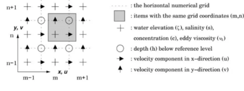
FIGURE 7.HORIZONTAL NUMERICAL GRID IN DELFT3D-FLOW; THE STAGGERED ARAKAWA C-GRID. 42

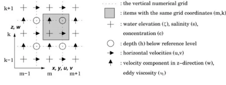
FIGURE 8.CARTESIAN (LEFT) AND Σ (RIGHT) COORDINATES, DEFINITION OF THE VERTICAL NUMERICAL GRID.THE INDEXING K OF THE

LAYERS IN THE Z MODEL RUNS IN OPPOSITE DIRECTION FROM THE Σ MODEL.PICTURE REPRODUCED FROM BIJVELDS (2001). 43

FIGURE 9.VERTICAL STAGGERED NUMERICAL GRID.HERE THE INDEXING K OF THE VERTICAL POINTS IS ACCORDING TO THE DEFINITION

IN THE Z GRID.FOR THE Σ GRID K RUNS IN OPPOSITE DIRECTION. 44

FIGURE 10.AREAL IMAGE OF THE STUDY SITE,SUSQUEHANNA FLATS, TAKEN IN 2015 WITH AN OVERLAPPING LAYER SHOWING

SUBMERGED AQUATIC VEGETATION DENSITY M ON THE BED (VIRGINIA INSTITUTE OF MARINE SCIENCE:

HTTP://WEB.VIMS.EDU/BIO/SAV/MAPS.HTML). 55

(6)

4

FIGURE 12.SCHEMATIZATION OF THE BED LEVEL CORRESPONDING TO THE STAGNANT BAR CONFIGURATION (RUN IDT11064) WITH

THE SEAGRASS DEPTH RANGE AND VELOCITY PROFILE IN THE DELFT 3D VEGETATION MODEL FOR SUBMERSED VEGETATION

(BAPTIST’S FORMULATION). 62

FIGURE 13.(A)BATHYMETRIC CONTOUR MAP OF THE STAGNANT CONFIGURATION AND VELOCITY MAGNITUDE VECTORS IN THE CASE

OF VEGETATED BAR (HV=0.4M; M=4M-1);(B) LONGITUDINAL U AND (C) TRANSVERSE V DEPTH AVERAGED VELOCITY ALONG

THE TRANSVERSE TRANSECT 400M, SECTION A, FROM THE RIVER MOUTH, FOR DIFFERENT VEGETATION HEIGHTS HV AND

DENSITY M COMPARED WITH THE NON-VEGETATED TEST CASE (SOLID BLACK LINE).THE LINES PARALLEL TO THE Y AXIS

DELIMIT THE RIVER MOUTH WIDTH. 65

FIGURE 14.(A)NORMALIZED LONGITUDINAL VELOCITY ALONG THE CENTERLINE COMPUTED WITH DIFFERENT CONDITIONS OF

VEGETATION.(B)RELATIVE DECAY OF THE AVERAGE VELOCITY S ALONG THE CENTERLINE AS A FUNCTION OF THE

VEGETATION HEIGHT FOR DIFFERENT VALUES OF DENSITY. 66

FIGURE 15.BED SHEAR STRESS CALCULATED ALONG THE CENTERLINE FOR DIFFERENT VEGETATION CONDITIONS PLOTTED AS A

FUNCTION OF THE LONGITUDINAL DIRECTION X (M) NORMALIZED BY THE RIVER MOUTH WIDTH W (M). 66

FIGURE 16.(A)SUSPENDED-SEDIMENT CONCENTRATION ON THE NON-VEGETATED BAR ALONG THE Z-DIRECTION (DEPTH) AND (B)

SUSPENDED-SEDIMENT CONCENTRATION ON THE VEGETATED BAR ALONG THE Z-DIRECTION (SUBMERGED VEGETATION

HEIGHT HV=0.4M, M=4M-1). 67

FIGURE 17.NORMALIZED-SUSPENDED SEDIMENT MASS ALONG THE CENTERLINE AS A FUNCTION OF VEGETATION HEIGHT FOR

DIFFERENT DENSITY SCENARIOS AND LINEAR REGRESSION LINES PLOTTED FOR EACH DENSITY. 68

FIGURE 18.(A)PLANVIEW MAP OF SIMULATED LOCATIONS OF THE NON-VEGETATED BAR (BLUE LINE) AND THE VEGETATED BAR (RED

LINE;HV=0.4M, M=4M-1) AFTER 63 DAYS OF SIMULATION FOR THE CONTOUR Z=-1M.THE GREEN SHADED REGION INDICATES THE INITIAL LOCATION OF THE BAR WITH THE VEGETATED PATCH (HV=0.4M, M=4M-1) AT THE SECTION Z=-1M. (B)BED LEVEL EVOLUTION OF THE VEGETATED BAR AND (C) NON-VEGETATED BAR EVERY TWO DAYS CALCULATED ALONG

THE CENTERLINE. 70

FIGURE 19.NORMALIZED BAR DISTANCE FROM THE RIVER MOUTH ALONG THE CENTERLINE AS A FUNCTION OF (A) VEGETATION

HEIGHT AND >(B) SEDIMENT GRAIN SIZE IN THE PRESENCE OF SUBMERSED VEGETATION CHARACTERIZED BY HV=0.4M AND

M=4M-1.THE RED CIRCLE MARKERS IN THE FIGURES REPRESENT THE SAME STUDY CASE. 71

FIGURE 20.SEDIMENT FLUX CROSSING THE BAR PEAK AS A FUNCTION OF THE TOTAL SUBMERGED VEGETATION VOLUME PER SQUARE

METER VV.THE RED MARK REPRESENTS THE TIPPING POINT AND THE BLACK DASHED LINE INDICATES THE SWITCHING TREND

OF THE BAR CROSSING THE TIPPING POINT. 72

FIGURE 21.BED LEVEL EVOLUTION WITH THE CORRESPONDING ACCRETION RATE OF SEDIMENT DEPOSITION AND EROSION DURING (A)

THE WINTER,(B) THE SPRING AND (C) THE SUMMER, VARYING THE INITIAL CONDITIONS OF SUSPENDED SEDIMENT CONCENTRATION, DISCHARGE AND THE PRESENCE OR ABSENCE OF SUBMERGED VEGETATION ON THE BAR;(D) PROGRESSIVE

(7)

5

BED LEVEL EVOLUTION DURING THE ALTERNATING SEASONS WITH THE CORRESPONDING ACCRETION RATE OF SEDIMENT

DEPOSITION AND EROSION FOR EVERY SEASON. 76

FIGURE 22.HISTORICAL BATHYMETRY OF SUSQUEHANNA FLATS (NAVIGATION CHARTS BY NOAA:

HTTP://HISTORICALCHARTS.NOAA.GOV/HISTORICALS) AND THE MEASURED BAR DISTANCE FROM THE SUSQUEHANNA RIVER

(8)

(9)

7

1. Introduction

The new paradigm that earth surface processes and landforms cannot be well understood without considering biological influences is becoming increasingly recognized within the geomorphological community (Howard and Mitchell, 1985; Naiman et al., 1988; Butler,

1995; Osterkamp and Hupp, 1996; Phillips, 1999; Gurnell et al., 2001; Stallins, 2006).

Several studies have shown how biological organisms can control physical processes within the fluvial environment (Tabacchi et al., 2000; Gurnell et al., 2005) while other studies have focused on how hydrogeomorphic processes and landforms can control biological communities (Naiman and Décamps, 1997; Steiger et al., 2005). However, there remains limited understanding of how the biogeomorphic processes lead to the reciprocal adjustments between landforms and biological communities which define the landscape dynamics.

The analysis of the reciprocal linkage between biological communities and geomorphic processes and landforms can be called ‘biogeomorphology’. Biogeomorphology is an emergent subdiscipline at the interface between ecology and geomorphology (Viles, 1988;

Naylor et al., 2002) which promotes the development of new interdisciplinary concepts,

models and methodological tools better adapted to break the biotic–abiotic dichotomy. The biological influence on geomorphological processes is the influence of biota to create, maintain or transform their own geomorphological surroundings. In some cases, morphological processes are dominant over biological processes and therefore the biota have to adjust to their environment. In other cases, biological processes are dominant. The most interesting are those cases where there is a mutual interaction that leads to feedback coupling of processes.

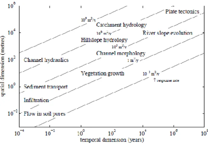
When looking for these cases, it is important to examine the temporal and spatial scales of the mutually interacting processes. Geomorphological processes occur on time scales ranging from microseconds, relevant to turbulence, up to hundreds of millions of years for geological processes. The spatial scale range is similarly wide, from micrometers for

(10)

8

capillary flows in sediments up to the continental and global scales. Kirkby (1990) presents an example for the wide variety in scales for river systems (Figure 1). He presents a measure for the response rate of systems, defined as a diffusive transport rate, i.e. the ratio of the squared spatial dimension (m2_{) over the temporal dimension (y). The response rates}

for morphological processes such as sediment transport, channel morphology and river slope evolution are of the same size (about 103 m2_{/y), irrespective of the scale order.}

Hydraulic and hydrologic processes also share a response rate, which is larger than for morphological processes (about 106 m2_{/y). Vegetation growth has a relatively small}

response rate (about 1 m2_{/y), meaning that changes in vegetation patterns are a less}

dynamic landscape element than changes in morphology.

Figure 1. Temporal and spatial scales for geomorphological processes. The response rate

indicates the evolution rate of the processes (Figure by Baptist, 2005).

As a general concept, this comparison of response rates may hold true for natural river systems. Consequently, this leads to the observation that for floodplain biogeomorphology,

(11)

9

morphodynamics is leading over vegetation dynamics and not the other way around. On the other hand, the reverse may be true in small, vegetation dominated streams.

Hydrologic, ecologic and geomorphic processes in a river basin are inherently coupled. On the one hand, natural vegetation patterns result from the interplay between climate, soils and topography; on the other, vegetation in turn exerts important controls on the hydrologic and geomorphic processes in the basin and contributes to the formation of landscape morphology over the long term. Vegetation is clearly an important factor in geomorphology.

Interactions between vegetation, hydrology and landscape development is inherently complex. It is conceivable that plant response to soil moisture deficit (Porporato et al.,

2001), plant suitability to climate and soil conditions (Laio et al., 2001; Porporato et al., 2003), and coexistence of different species and functional types (van Wijk and Rodriguez-Iturbe, 2002; Fernandez-Illescas and Rodriquez-Rodriguez-Iturbe, 2004) would have important

implications for erosion rates and resulting landscape morphology. However, using a simple vegetation growth function seems to be a relevant preliminary strategy, although it will be applicable only in regions where plant growth is not limited by water. A number of fundamental questions in the interface between ecology and geomorphology remain to be explored.

1.1 Problem description

Coastal and estuarine modeling is concerned with understanding and predicting marine processes in coastal oceans and estuaries. One component of coastal and estuarine modeling is the prediction of sediment transport, including both fine sediments in shallow estuaries and coarser sediments in near-shore, wave-driven environments.

Over long time scales, sediment transport governs morphodynamics which strongly impacts coastal and estuarine flows. Unique to coastal and estuarine modeling is the connection to human influences particularly in densely populated coastal regions, where flows can be altered by coastal structures, dredging and sand nourishment operations, and

(12)

10

anthropogenic sources of contaminants and nutrients significantly impact coastal biogeochemistry.

Given that roughly 60% the world’s population lives within 60 km of the coast and this is expected to rise to 75% within a few decades (Rao et al., 2008), accurate coastal and estuarine modeling is an essential component of efficient management for the sustainability of natural coastal systems and the development and improvement of sustainable urban infrastructure, particularly in the face of rapid urbanization of coastal cities and changing climate including sea-level rise.

This work focuses on the effect of vegetation on the development of a river mouth bar. The area in front of the mouth of deltaic distributary channels and rivers is a location where sediments accumulate and new landforms. At these locations sediment deposition can occur by growth of natural levees and channel elongation or by deposition and vertical aggradation of mouth bars.

Irrespective of their shape and evolution, these landforms are of paramount importance within the coastal landscape because, after emerging, they become deltaic islands and subaerial levees, which protect coastal communities (Costanza et al., 2008) and provide habitat for rich and productive ecosystems (Gosselink and Pendleton, 1984). In general, land naturally builds and erodes in relation to switching depocenters of rivers debouching in the ocean and sea level oscillations over long timescales, and storms and river floods over shorter timescales. In recent decades several river mouth landforms have been deteriorating because of sediment starvation triggered by the damming of large rivers, which reduces the flux of sediments to the ocean (Syvitski et al., 2005). In a period in which sea level rise is enhancing coastal erosion and flooding (Nicholls and Mimura, 1998), it is more important than ever to understand the physics of river mouth sediment deposits and how new land is built. In fact, deposition of sediments at river mouths not only can mitigate coastal erosion but it can also promote land expansion thus restoring anthropogenically modified coastlines (Paola et al., 2011; Nittrouer et al., 2012; Edmonds, 2012, Kim et al.,

2009; Kim, 2012).

The formation of a bar, its size and shape depend on the intensity of sea and freshwater interaction processes taking place at the mouth of a river.

Bars are usually formed under similar environmental factors and the bar features can be traced at almost any river mouth. To form a bar in the mouth of a river, it is sufficient to

(13)

11

have a water flow that can transfer river sediments. The action of the river water flow and the sediment discharge builds up a background upon which the effect of other factors, such as waves, tidal currents, sea level rise, etc., deforming and shaping an already formed bar, is displayed. There is no doubt that passive factors as coastline configuration, sea-bottom relief underlying the bar, geological structure, etc., play no less an important role in the bars formation.

The growth of vegetation on the top of the sediment formations built up by a river flow enables them to consolidate. While hampering the further movement of sediments carried by the river flow, the vegetation cover facilitates the bar development, promotes the bifurcation of the river channel and contributes to the grows. This work is inspired by the sudden resurgence of the submersed aquatic vegetation (SAV) bed in the Chesapeake Bay (USA). Because the SAV bed occurs at the mouth of the Bay’s main tributary (Susquehanna River), it plays a significant role in modulating sediment inputs from the Susquehanna to the Bay.

1.2 Objective and research questions

The objective of this thesis is to obtain a better understanding of the effect of vegetation on the development of river mouth bars. To reach this objective, four research questions are given below. Combined, these questions will set a next step in understanding vegetated flows and sediment transport in vegetated flows.

1. What are the factors influencing river mouth bars formation and development in absence of vegetation?

2. How can a numerical experiment be designed to make relevant observation on sediment transport in and around vegetation, combining long term processes (morphology) with small-scale effects (vegetation)?

(14)

12

3. What is the influence of submersed vegetation on the hydrodynamics and sediment transport of a river mouth bar?

4. Is it possible to explain bars growth patterns from submersed vegetation characteristics?

1.3 Outline

Chapter 2 gives the literature study and some background information starting with an overview of the effect of vegetation on the flow and specific aspects that influence the roughness and the turbulence. The literature gradually zooms into the fluid mechanics at the scale of an individual patch of vegetation examining turbulence and velocity profile of a flow through vegetation. This chapter also covers sediment transport mechanism, important for flow through vegetation. Furthermore, the state of the art of numerical models of flow-vegetation interaction is illustrated.

The method used for the numerical experiment is explained in chapter 3, focusing on the governing equations, some numerical aspects of the model and the vegetation model used in this study.

The numerical setup and the result analysis are explained in chapter 4. Figures and tables support the understanding of the numerical experiments.

The results are discussed in chapter 5 providing a comparison with previous river mouth models. In addition, seasonality effects on river mouth bar morphodynamics is analyzed. This chapter also reflects on the applicability of this results on the real case of Susquehanna Flats and other study systems. The last chapter gives the conclusions of this research.

(15)

13

2. Literature and theoretical frameworks

Vegetation is one of the important waterway components that play a key role in the flow and transport. Recently, developments in the field of river and coastal management have led to renewed interest in retaining the vegetation due to costly and ecological damaging procedures of removing channels vegetation.

Vegetation has shown positive impacts on water quality by removing pollution, increasing bed stability, assisting river restoration/rehabilitation, maintaining aquatic ecosystems, controlling flow velocity, improving rivers geomorphology, decreasing bed load and turbidity, diversifying habitat, as well as capturing and sequestering carbon (Schulz et al.,

2003; Sim et al., 2008; Jarvela, 2004; Afzalimehr and Dey, 2009; Arroyave and Crosato ,2010; Liu and Shen, 2008; Folkard, 2011). Moreover, vegetation improves bank stability through

sediment root binding, which increases the threshold shear stress, required to gradually wash the sediment.

Moreover, vegetation offers local flow resistance by reducing velocity, because it increases drag, while simultaneously decreasing the availability of shear stress for transport and erosion (Thorne, 1990; Carollo et al,. 2002). Ffolliott et al. (1995) have demonstrated that unprotected channels are more susceptible to erosion than channels protected by using a vegetative cover or lining. As soon as there is erosion in a channel, it becomes difficult to control it. The management of flood and river engineering requires the understand the effects of vegetation on the flow rate and sediment transport, which also determines the retardation in channels that are crucial in restoration design works (Jarvela, 2005; Nepf

and Ghisalberti, 2008).

Chezy, Darcy-Waisbach and Manning formulations are equations generally used for flow resistance. A roughness coefficient which quantifies the flow resistance is considered in these formulas. Specifying the effect of vegetation in these relations has been attempted by researchers (Jarvela, 2005; Afzalimehr and Dey, 2009). However, the first analyses and discussion on vegetated channels was published in the last century by Chow (1959) and Barnes (1967), with definitions on semi-empirical methods for estimating the flow resistance.

The most widely used resistance measure is the flow resistance coefficient, Manning of vegetated channels. Gardiner and Dackombe (1983) have shown the use of traditional

(16)

14

methods for channel resistance as component parts, which uses experimental tables to value every element separately before determining the final value for the Manning’s. However, the resistance tables used was very subjective and the estimated coefficient may be highly inaccurate (Hey, 1979) because flow resistance was presented as a function of the vegetation size, their location in the channel, the local flow conditions and structural properties (Green, 2005).

Darby (1999), Green (2005), and Jarvela (2005) however stated that when additional vegetation factors are introduced which include stems flexibility, plant height, and vegetation porosity, there is the likelihood that resistance tables become more inaccurate. Natural vegetation behaves different compared to artificial vegetation, for example, aquatic plants are difficult to bend during the day and period of growth because of the increase in the production of photosynthetic oxygen, which increases their boundary (Powell, 1978), seasonal vegetation effectiveness (Fisher, 1992) or age (Pitlo, 1986). Moreover, most figures and tables of resistant coefficients were not specifically designed for vegetated channels, and therefore, underestimate their resistance values (Charnley, 1987). Afzalimehr and Dey (2009) have stated that the vegetation environment representing the area under the coverage of the vegetation, is a very important component in vegetated channels because it has significant impact on the turbulence of flow (Folkard, 2005), velocity (Jarvela, 2004), and sediment transport rate (Zong and Nepf, 2010). Nepf and Ghisalberti (2008) have stated that majority of the studies on vegetation focused on continuous beds, although in many natural settings, vegetation occurs in discontinuous patches of finite length. Afzalimehr and Dey (2009) has demonstrated different velocity profiles for some vegetation types, which conforms with previous studies (Folkard, 2005;

Wang et al., 2009). However, several researches have demonstrated different turbulent

behavior for various vegetation distribution and patches positions (Zong and Nepf, 2010;

(17)

15

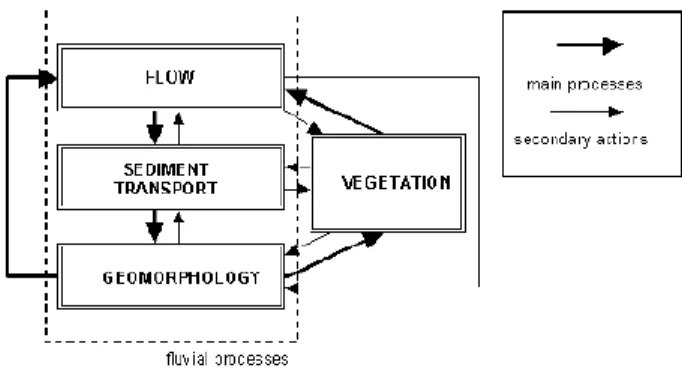
Figure 2. The influence of vegetation on fluvial processes (Baptist, 2005).

2.1 Flow through vegetation

2.2.1 Emergent vegetation

An emergent canopy fills the entire water depth H and typically penetrates the water surface.

This type of canopy occurs in tidal marshes, kelp forests, and seagrass meadows during periods of low tide.

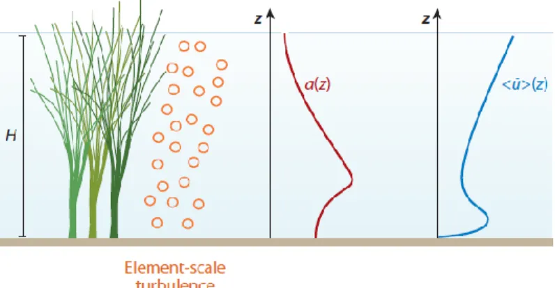
Emergent canopies impose structure on both the mean and turbulent flow over the entire water column. The canopy dissipates eddies with scales greater than the stem scales, while contributing additional turbulent energy at these stem scales (Figure 3).

As a result, the dominant turbulent length scale within a canopy is shifted downward from analogous conditions without vegetation. In a channel with rigid vegetation, the integral length scale of the turbulence, is set by the smaller of the stem diameter or the average distance to the nearest neighboring stem, regardless of the water depth (Tanino & Nepf,

(18)

16

Figure 3. Emergent canopy of marsh grass, with vertical (z) profiles of leaf area index, a,

and longitudinal velocity, <u¯>. The velocity profile varies inversely with a, creating a velocity maximum close to the bed, below the level at which branching begins.

In a square array of stems, the average spacing and the average nearest neighbor spacing are the same, but not in a random array. When the stem diameter is less than the average distance between stems, turbulence is generated within stem wakes (if the Reynolds number is sufficient) so that the length scale is equal to the stem diameter.

Otherwise, turbulence is generated within the pore channels. Even for solid volume fractions as low as 0.6%, the production of turbulence by the canopy exceeds the production by the bed shear over most of the flow depth (Nepf et al., 1997; Burke &

Stolzenbach, 1983; Lopez & Garcia, 1998).

Therefore, the turbulence level cannot be predicted from the bed-friction velocity, as it can for

open-channel flow. Instead, it is a function of the canopy drag. Vortex generation by stem wakes and/or in pore channels drains energy from the mean flow (expressed in terms of canopy drag) and feeds it into the turbulent kinetic energy. If this conversion is 100% efficient, then the rate at which turbulent energy is produced, PW, is equal to the rate at

which mean flow energy is extracted, i.e., the rate of work done by the flow against canopy drag (Raupach & Shaw, 1982):

(19)

17

𝑃𝑤=

1 2𝐶𝐷𝑎(𝑢̅)

3_{Eq. 1}

In fact, only the form drag is converted into turbulent kinetic energy. The viscous drag component is immediately dissipated to heat. For stiff canopies, i.e., most emergent canopies, and Re>200, the majority of the drag is form drag, and PW is a reasonable

approximation (Tanino & Nepf, 2008). In contrast, Nikora&Nikora (2007) suggested that for flexible canopies, which are typically submerged, the drag is predominantly viscous, and previous equation would be an overestimate of stem-scale turbulence production. The relative contributions of viscous drag and form drag depend on the morphology and alignment of the blades and stems within the canopy.

Within a homogenous emergent canopy, transport terms are negligible, and the wake production is balanced by viscous dissipation, ε, i.e., PW = ε.

In addition, for turbulent kinetic energy, k, the dissipation rate within the canopy has the scale (Tennekes & Lumley, 1972)

𝜀~(𝑘̅)3/2_𝑙−1_{Eq. 2}

Connecting the equations, the turbulent intensity in the canopy is

√(𝑘̅ ) (𝑢̅) ~(𝐶𝐷𝑎𝑙)

1/3_{Eq. 3}

The turbulence length scale, l is set by the smaller of the stem diameter, d, and the nearest-neighbor stem spacing, Sn. In a canopy of low solid volume fraction, or specifically Sn > d,

the turbulence intensity increases rapidly with increasing canopy density because l= d, and thus al ≈ d2_/S_n2_{. In a canopy of high solid volume fraction, S}_n_{< d, the turbulence intensity}

increases more slowly because l= Sn, and thus al ≈ d/Sn.

Within an emergent canopy, the momentum equation will generally simplify to a balance between potential forcing and canopy drag. Viscous stress is negligible compared to

(20)

18

vegetative drag over most of the depth, excluding a thin layer near the bed of a scale comparable to the stem diameter, d (Nepf & Koch, 1999). Then, the eddy length scale is small compared to the water depth, which limits the turbulence flux of momentum; i.e., the turbulence stresses are typically negligible. For example, from numerical experiments, the eddy scales are 1%–3% of the water depth, and turbulent stresses are only 2% of the total drag for aH = 0.1 (Burke & Stolzenbach, 1983). Similar ratios have been measured in model emergent canopies (Nepf & Vivoni, 2000). A notable exception occurs near the surface, as wind-generated stress can sometimes play a role in the momentum balance (Jenter & Duff,

1999). Third, we assume that dispersive fluxes are negligible because the canopy density

is commonly above the threshold ah > 0.1 suggested by Poggi et al. (2004). For steady, uniform flow, the momentum equation then reduces to

𝑔 (𝜕𝐻 𝜕𝑥+ sin 𝜃) = − 1 2 𝑎𝐶𝐷 1−𝜑(𝑢̅)|(𝑢̅)| = − (𝑢̅)|(𝑢̅)| 𝐿𝑐 Eq. 4

The hydrostatic pressure and potential gradients that drive the flow are not functions of the vertical coordinate, z. The right-hand side then must also be independent of z so that the velocity varies inversely with the frontal area, a, and in proportion to the canopy drag length scale, Lc.

For plants with a distinct basal stem, this produces a velocity maximum close to the bed because a is reduced below the level at which branching begins. A near-bed velocity maximum is often observed in the marsh grass Spartina alterniflora (Leonard & Luther,

1999;, Leonard & Croft, 2006). In contrast, the more vine-like Atriplex portulacoides has

leaves that are more evenly distributed over depth, and the resulting velocity profile is uniform over depth (Leonard & Reed, 2002).

The velocity profile within an emergent canopy has a similar form.

When the velocity is normalized by its value at an arbitrary reference depth, denoted by the subscript ref, the normalized profiles collapse together, regardless of the absolute magnitude of the current. The shape of the normalized profile depends on the vertical distribution of Lc: (𝑢̅) (𝑢̅)𝑟𝑒𝑓= √ 𝐿𝑐 𝐿𝑐−𝑟𝑒𝑓~√ (𝐶𝐷𝑎)𝑟𝑒𝑓 (𝐶𝐷𝑎) Eq. 5

(21)

19

where the right-most approximation holds in most salt- and freshwater wetlands canopies, for which the canopy solid volume fraction is small (φ < 0.1) so that (1 − φ) ≈ 1. A similar velocity structure was confirmed by measurements in a coastal marsh (Lightbody

& Nepf, 2006) and in the freshwater wetlands of the Everglades (Huang et al., 2008). The

normalization provides an important tool for extrapolating a full velocity profile from records at a single vertical position.

An interesting nonlinear behavior emerges comparing flow conditions under different canopy densities but with the same potential and/or pressure gradient.

To include the no-canopy limit (i.e., bare bed), one must incorporate the bed resistance into the momentum balance.

Because the vegetation offers additional resistance, the velocity within the canopy is always less than that over a bare bed, and the velocity ratio, (𝑢̅)/𝑢𝑏 , decreases as the

vegetation density increases. Changes in turbulent kinetic energy with increasing vegetation density reflect the competing effects of the reduced velocity and the additional turbulence production in stem wakes. These opposing tendencies produce a nonlinear response in which the turbulence levels initially increase with increasing canopy density but decrease as a increases further. This nonlinear response was predicted numerically for flow through emergent vegetation (Burke & Stolzenbach, 1983) and within submerged roughness elements (Eckman, 1990). It has been observed in flume studies of flow through real stems of Zostera marina (Gambi et al., 1990). The enhanced turbulence levels in sparse canopies have important implications for canopy ecology.

It is commonly expected that dense patches of vegetation, because they damp flow and turbulence, are associated with muddification, an increase in fine particles and organic content of the underlying sediment relative to adjacent bare-bed conditions. Recently, van Katwijk et al. (2010) observed that sparse patches of vegetation are associated with sandification, a decrease in fine particles and organic matter, and they attribute this to higher levels of turbulence within the sparse patch, relative to adjacent bare regions. A transition from a tendency for sandification (elevated turbulence) to a tendency for muddification (diminished turbulence intensity) with increasing canopy density is consistent with the nonlinear model.

(22)

20

2.2.2 Submerged vegetation

The velocity within a submerged canopy has a range of behavior depending on the relative depth of submergence, defined as the ratio of flow depth H, to canopy height, h. The flow within the canopy is driven by the turbulent stress at the top of the canopy as well as by the gradients of pressure and gravitational potential (bed slope).

The relative importance of these driving forces varies with the depth of submergence (Nepf

& Vivoni, 2000):

𝑡𝑢𝑟𝑏𝑢𝑙𝑒𝑛𝑡 𝑠𝑡𝑟𝑒𝑠𝑠 𝑝𝑟𝑒𝑠𝑠𝑢𝑟𝑒 𝑔𝑟𝑎𝑑𝑖𝑒𝑛𝑡~

𝐻 ℎ− 1

Three classes of canopy flow can be defined: deeply submerged or unconfined (H/h > 10), shallow submergence (H/h < 5), and emergent (H/h = 1).

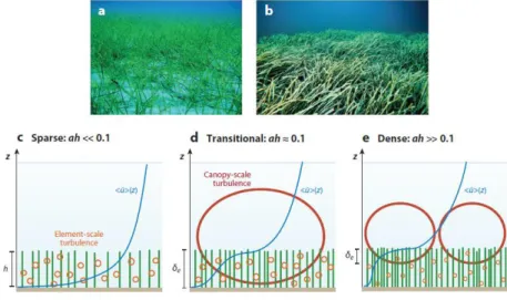
Figure 4. (a) The seagrass Cymodocea nodosa at low stem density. (b) The seagrass

(23)

21

profiles of longitudinal velocity and dominant turbulence scales are shown for (c) a sparse canopy (ah<<0.1), (d) a transitional canopy (ah ≈ 0.1), and (e) a dense canopy (ah>>0.1), where h is the submerged canopy height. For ah ≥ 0.1, a region of strong shear at the top of the canopy generates canopy-scale turbulence. Element-scale (stem-scale) turbulence is generated within the canopy.

A great deal is known about unconfined canopy flow based on work in terrestrial canopies (Raupach et al., 1996; Finnigan, 2000; Belcher et al., 2012). When unconfined, the flow within a canopy is driven by the turbulent stress at the top of the canopy, i.e., by the vertical turbulent transport of momentum from the overflow, with negligible contribution from pressure gradients. The terrestrial canopy model can be applied to aquatic canopies that are deeply submerged. However, because of the limitation of light penetration, most submerged aquatic canopies occur in the range of shallow submergence H/h<5 (Chambers&Kalff, 1985; Duarte, 1991), for which both turbulent stress and potential gradients are important in driving flow in the canopy. For emergent conditions (H/h=1), flow is driven by the potential gradients, as described in the previous section. For a submerged canopy, there are two limits of behavior, depending on the relative importance of the bed drag and the canopy drag. If the canopy drag is small compared with the bed drag, then the velocity follows a turbulent boundary-layer profile, with the vegetation contributing to the bed roughness (sparse canopy; Figure 4c). If the canopy drag is large compared to the bed drag, the discontinuity in drag that occurs at the top of the canopy (z = h) generates a region of shear resembling a free shear layer with an inflection point near the top of the canopy (dense canopy; Figure 4d,e). From scaling arguments, Belcher et al. (2003) predicted that the transition between the sparse and dense regimes occurs at the roughness density λf = ah = 0.1. Numerical simulations by Coceal & Belcher (2004) suggest

that the transition occurs at Lc/h = 5, which corresponds to λf = 0.15, for their parameter

set (CD = 2, φ = 0.25). On the basis of measured velocity profiles in aquatic systems (Nepf

et al., 2007), the profile exhibits a boundary-layer form with no inflection point if

CDah<0.04. A pronounced inflection point appears at the top of the canopy for CDah>0.1.

Because CD ≈ 1 in most of the studies considered, these limits are consistent with the scaling

and numerical estimates given above.

For dense canopies, Raupach et al. (1996) demonstrated a similarity between canopy shear layers and free shear layers. In a free shear layer, the velocity profile contains an inflection

(24)

22

point, which triggers a flow instability that in turn leads to the generation of Kelvin-Helmholtz vortices (Brown & Roshko, 1974; Winant & Browand, 1974). These structures dominate the transfer of momentum between the high-speed and low-speed streams, and their size sets the length scale of the shear layer. For dense submerged canopies (ah≥0.1), the momentum absorption by the canopy is sufficient to produce an inflection point in the velocity profile, which, as in free shear layers, leads to the generation of Kelvin-Helmholtz vortices (Figure 4d,e). These vortices are called canopy-scale turbulence to distinguish it from the much-larger boundary-layer turbulence, which may form above a deeply submerged or unconfined canopy, and the much smaller stem-scale turbulence.

Over a deeply submerged canopy (H/h>10), the canopy-scale vortices are highly three-dimensional owing to their interaction with the larger boundary-layer turbulence, which stretches the canopy-scale vortices, enhancing secondary instabilities (Fitzmaurice et al.,

2004, Finnigan et al., 2009). However, with shallow submergence (H/h≤5), which is

common

in aquatic systems, larger-scale boundary-layer turbulence is not present, and the canopy-scale vortices dominate the turbulence field, both within and above the canopy (Ghisalberti

& Nepf, 2005; 2009). For shallow submergence, the canopy-scale turbulence is also more

coherent than that observed with deeply submerged conditions. However, in both cases, the canopy-scale vortices dominate the vertical transport at the canopy interface (Gao et

al., 1989; Finnigan, 2000; Ghisalberti & Nepf, 2002).

In a free shear layer, the vortices grow continually downstream, predominantly through vortex pairing (Winant&Browand, 1974). In canopy shear layers, however, the vortices reach a fixed scale and a fixed penetration into the canopy (δe in Figure 4d,e) at a short

distance from the canopy’s leading edge (Ghisalberti & Nepf, 2004). On the basis of measurements with a flexible model of the seagrass Z. marina (a = 5.7 m−1), a fixed shear-layer scale is reached at a distance of 10h from the leading edge of the meadow (Ghisalberti,

2000). The fixed vortex and shear-layer scale is reached when the shear production that

feeds energy into the canopy-scale vortices is balanced by dissipation by canopy drag. This energy balance predicts the following length scale, which has been verified by laboratory observations (Nepf et al., 2007):

𝛿𝑒=0.23±0.6_𝐶

(25)

23

In the range CDah = 0.1 to 0.23, the shear-layer vortices penetrate to the bed, δe=h, creating

a highly turbulent condition over the entire canopy height (Figure 4d). At higher values of CDah, the canopy-scale vortices do not penetrate to the bed, δe <h (Figure 4e).

The scaling δe ∼ a−1 has been observed in flows near porous layers over a wide range of

physical scales, from granular beds to terrestrial forests and urban canopies (Ghisalberti,

2009). However, the scale relation must break down when (CDa)−1 approaches the scale of

the canopy elements, d, because a is defined only as an average over multiple elements. For rigid cylinders, when (CDa)−1 is less than 2d, the penetration scale transitions to a constant

δe ≈ 2d (White & Nepf, 2007). The depth of submergence, H/h, can also affect the

penetration length scale. For H/h < 2, δe is diminished, as interaction with the water

surface diminishes the strength and scale of the vortices (Nepf & Vivoni, 2000; Okamoto &

Nezu, 2009).

The penetration length, δe, segregates the canopy into an upper layer of strong turbulence

and rapid renewal and a lower layer of weak turbulence and slow renewal (Nepf & Vivoni,

2000). Flushing of the upper canopy is enhanced by the canopy-scale vortices that

penetrate this region (Figure 4e). In contrast, turbulence in the lower canopy (z < h − δe) is generated in stem wakes and has a significantly smaller scale, set by the stem diameters and spacing. Canopies for which δe/h<1 (Figure 4e) shield the bed from strong turbulence

and turbulent stress.

Because turbulence near the bed plays a role in resuspension, these dense canopies are expected to reduce resuspension and trap sediment. Consistent with this, Moore (2004) observed that resuspension within a seagrass meadow was reduced, relative to bare-bed conditions, only when the above-ground biomass per unit area was greater than 100 gm−2

(dry mass). This biomass corresponds to ah = 0.4 (Luhar et al., 2008). The transition in near-bed turbulence and resuspension does not occur abruptly at CDah = 0.23 but occurs

gradually with increasing CDah above this value, as the canopy-scale vortices are

progressively pushed further from the bed (Nepf, 2011). Because of the reduced near bed turbulence, dense canopies can promote sediment retention. In sandy regions, which tend to be nutrient poor, the preferential retention of fines and organic material (muddification) enhances the supply of nutrients to the canopy so that dense canopies provide a positive feedback to canopy health in sandy regions. In contrast, in regions with muddy substrate,

(26)

24

sparse meadows (CDah≤0.23) may be more successful because the enhanced near-bed

turbulence removes fines, leading to a sandier substrate.

2.2.3 Velocity profile

Sufficiently far above a submerged canopy (z > 2h), the velocity profile is logarithmic (Kaimal & Finnigan, 1994):

(𝑢̅) =𝑢∗

𝑘𝑙𝑛 (

𝑧−𝑧𝑚

𝑧0 )

Eq. 7

with κ = 0.4 (von Karman constant). The horizontal average is not strictly needed above the canopy but is retained for consistency with the equations within the canopy. The friction velocity, u∗, is related to the Reynolds stress at the top of the canopy, 𝑢∗2=< 𝑢′𝑤′̅̅̅̅̅̅ > ℎ .

The parameters zm and zo are the displacement and roughness heights, respectively, both

of which depend on the canopy roughness density, ah. On the basis of studies with both model and real vegetation, a simple estimate for friction velocity is u* = [gS(H − h)]0.5, with

S=∂H/∂x +sinθ (Murphy et al., 2007). If the vegetation is flexible, then h is the mean deflected height of the canopy ( Jarvela, 2005). However, if the depth of submergence is small, compared to the displacement height, the following estimator is more accurate: u*=[gS(H−zm)]0.5 (Nepf & Vivoni, 2000).

Remembering that the penetration length scale, δe, describes the distance over which

turbulent stress penetrates the canopy from above., similarly, the displacement height is the centroid of momentum penetration into the canopy (Thom, 1971). This similarity suggests the physically intuitive scaling

𝑧𝑚 ℎ ~1 − 1 2 𝛿𝑒 ℎ = 1 − 0.1 𝐶𝐷𝑎ℎ Eq. 8

(27)

25

which has been confirmed for ah ≈ 0.2 to 3 (Luhar et al., 2008). For ah > 1, the displacement thickness tends toward zm ≈ h, indicating that essentially the entire canopy is cut off from

the overflow. In addition, zm goes to zero at ah = 0.1. When zm = 0, the velocity profile has no

inflection point (Figure 4c), consistent with the observation that ah > 0.1 is required to produce an inflection point in measured velocity profiles (Figure 4d, e).

The dependency of the roughness height, zo, on the canopy density, ah, differs significantly

above and below the threshold of ah = 0.1 (Raupach et al., 1980; MacDonald et al., 1998;

Jimenez, 2004; Luhar et al., 2008).

In the sparse-canopy range (ah < 0.1), the roughness height increases with increasing ah. In sparse canopies, the flow penetrates the full canopy so that zo is proportional to the drag

imparted by the full canopy, CDah, i.e., zo/h ∼ CDah.

In contrast, for dense canopies (ah > 0.1), the roughness height decreases with increasing ah. The effective height of the canopy, as seen by the overflow, is the penetration scale, δ

e. The roughness height depends on this effective height, rather than the canopy height, so

that zo∼δe ∼ a−1. For example, data summarized by Luhar et al. (2008) suggest that for ah

> 0.1, zo= (0.04±0.02)a−1.

The logarithmic profile form is based on equilibrium turbulence such that dissipation and production are locally in balance (Tennekes & Lumley, 1972). Largely because of the vertical transport provided by the shear-layer structures, this condition is not met for some distance above the canopy, called the roughness sub-layer. For very shallow submergence, H/h ≤ 1.5, the roughness sub-layer extends to the surface, and a logarithmic structure is not observed above the canopy.

The flow within a submerged canopy is driven by a combination of the turbulent, dispersive, and viscous stresses generated by the overflow, as well as the potential gradient associated with the hydrostatic pressure gradient and the bed slope. Below the penetration of turbulent and dispersive stress (z < h − δe), conservation of linear momentum reduces

to a balance between potential gradients and the sum of the canopy and the bed drag. Assuming that the canopy drag is much larger than the bed drag, this balance yields the following mean velocity:

(28)

26 (𝑢̅) = 𝑈1= √ 2𝑔(𝜕𝐻 𝜕𝑥+sin 𝜃) 𝐶𝐷𝑎 Eq. 9

This is the same momentum balance observed for emergent canopies. So, if the canopy density a or drag coefficient CD is a function of z, the velocity will vary inversely; i.e., the

velocity will be highest where CDa is lowest.

In the upper canopy (h − δe < z < h), flow is driven by both potential gradients and

turbulent stress. The stress-driven component is derived by simplifying the momentum equation to a balance of the canopy drag and turbulent stress and modeling the turbulent stress with a mixing length model, (𝑤_{̅̅̅̅̅̅) = 𝑙}′_𝑢′

𝑚2(𝜕 < 𝑢̅ > 𝜕𝑧)2 (Inoue, 1963).

This yields the exponential velocity profile observed in terrestrial canopies. In aquatic canopies, the potential-driven component is also important in the upper canopy. Combining the stress driven and potential-driven components, the upper canopy velocity profile is

(𝑢̅) = 𝑈1+ (𝑈ℎ− 𝑈1) exp[−𝐾𝑢(𝑏 − 𝑧)] Eq. 10

with Uh = (𝑢̅) at the top of the canopy, and constant Ku = β/lm, with β = u∗ /Uh. It is

physically intuitive that the mixing length should be related to the penetration of shear-layer vortices into the canopy.

For rigid canopies in water, β = 0.24 ± 0.02 (Ghisalberti & Nepf, 2005), which predicts Ku

= (8.7 ± 1.4)CDa. This predicted value agrees with the observed decay scale constant, Ku =

(9 ± 2)CDa, extracted from measured velocity profiles in Ghisalberti (2005). In the dense

canopy limit, β has no dependency on the canopy density (Ghisalberti & Nepf, 2005), but it declines as the transition to the sparse canopy limit (ah<0.1) is approached, i.e., as the canopy-scale vortices diminish and eventually disappear (Poggi et al., 2004b). Flexible canopies display a lower value, β = 0.17 ± 0.01 (Ghisalberti & Nepf, 2005), consistent with the less efficient momentum transfer noted in Figure 5. Belcher et al. (2003) proposed the alternative Ku=(2lm2Lc )−1/3, with the approximation lm  h.

(29)

27

Figure 5. Measured velocity (dots) from Ghisalberti (2005). Predicted velocity (solid line)

with confidence limits (dashed lines): H = 46.7 cm, h = 13.9 cm, S = 2.5 × 10−5_{, a = 0.034}

cm−1_{, and C}_D_{= 0.77 (measured). Above the meadow, the velocity is predicted from the}

logarithmic profile, with u∗ = [gS(H − h)]0.5, zm = h − (1/2) δe , and zo = (0.04 ± 0.02)a−1.

Inside the meadow, the velocity is predicted with Uh taken from logarithmic fit.

To model the full velocity profile, both within and above the bed, researchers have combined the models for above-canopy and in-canopy profiles by matching the velocity at the top of the canopy (Carollo et al., 2002; Abdelrhman, 2003). Although this ignores the roughness sub-layer, for practical purposes the resulting profile is reasonably accurate. First, the velocity profile above the meadow (z>h) is estimated from the logarithmic profile. The logarithmic

profile provides the velocity at the top of the meadow, Uh, which is used to predict the

velocity within the meadow (z < h). Other models for the complete velocity profile in regions with submerged aquatic vegetation have utilized different turbulence closure schemes (Shimizu & Tsujimoto, 1994; Lopez & Garcia, 2001; Poggi et al., 2004; Defina & Bixio,

2005), and some reflect the bending response of flexible vegetation (Abdelrhman, 2007; Dijkstra & Uittenbogaard, 2010).

2.2 Density and spatial distribution

Under natural conditions, plants often form spatially heterogeneous communities— patches which together with non-colonized spaces, or spaces colonized by different types

(30)

28

of vegetation, form irregular mosaics. Although the patchiness of aquatic vegetation is presently an important topic of ecological research (Nikora, 2010a; Vandenbruwaene et al.,

2011; Zong and Nepf, 2011).

The occurrence of patches in channels may transform relatively two-dimensional open channel flow into complex three-dimensional flows (Sukhodolov and Sukhodolova, 2010;

Siniscalchi et al., 2012). In fact, the flow patterns must be considered taking into account

the large-scale turbulence associated with flow separation and wakes at the patch scale (pattern #7, Fig. 6), boundary layers and mixing layers developing at the patch side (pattern #8, Fig. 6b), as well as interacting vertical (pattern #9, Fig. 6a) and horizontal boundary layers at the patch mosaic scale (Nikora, 2010; Zong and Nepf, 2010; Sukhodolov

and Sukhodolova, 2012).

Studies with submerged patches spanning the channel width showed that the upstream part of the patch diverts the flow upwards over the patch resulting in decelerating flow velocities in the canopy and flow acceleration above the patch.

This velocity difference contributes to the formation of a shear layer (Ghisalberti and Nepf,

2004; Sukhodolova and Sukhodolov, 2012) enhancing vertical turbulent transport of

momentum (Okamoto and Nezu, 2013; Zeng and Li, 2014). Moreover, such a flow feature suggests that plants at patch edges experience significantly larger drag than plants in the middle of the patch as they are exposed to larger flow velocities (Nikora, 2010; Siniscalchi

(31)

29

Figure 6. Flow patterns at patch scale: (a) side view considering patch mosaic structure

and (b) plan view at patch scale (from Nikora, 2010)

The patch density and geometry are dominating factors for the turbulent flow field in and around the patches (Green, 2005; Sukhodolov and Sukhodolova, 2012). Increasing the vegetation density results in faster development of velocity and turbulence inside the patch due to the larger resistance compared to sparse densities (Soulioutus and Prinos, 2011). Moreover, these in-canopy flow features develop faster than the flow characteristics above the canopy (Zeng and Li, 2014).

Vegetated patches represent porous patches and this porosity affects the wake flow conditions. For example, the resulting wake from a porous patch is much longer compared to the wake generated by a similar solid obstruction as the bleed flow delays the onset of the von Karman vortex street (Nepf, 2012).

In the case of emergent patches, the flow is deflected sideways from the patch and a shear layer develops at the interface between the patch and the free flow (pattern #8 in Fig. 6b). The resulting horizontal mixing layer eddies dominate mass and momentum exchange and affect both the open channel and canopy turbulent flow features (Nepf, 2012). The horizontal penetration depth of these eddies depends, as for the submerged canopy case, on canopy density. However, due to the significant differences in flow geometry, both cases cannot be directly compared (Nepf, 2012a). The presence of more than one patch, patch mosaics, can result in a hydrodynamic interaction so that the upstream patch affects the flow features of the downstream patch. Flow interaction between vegetated patches such as flow acceleration depends on the ratio of patch size and distance between patches (Vandenbruwane et al., 2001).

2.3 Sediment transport in vegetated flows

Few studies have examined the influence of vegetation on flow and morphological changes. Bennett et al. (2008) extended their research (Bennett et al., 2002) by performing experimental and numerical simulations to investigate channel responses to finite patches, which consisted of emergent and circular cylinders. They showed that channel alterations

(32)

30

caused by both bank erosion opposite the patches and local scour pools near the patches were affected significantly by vegetation density. However, the authors did not measure bed elevation within the patch because of limitations in the experimental conditions. Furthermore, Bouma et al. (2007) investigated spatial sedimentation patterns within patches in an intertidal flat. The patches comprised bamboo canes and two patch densities (low and high) were tested. Following 2 years of field monitoring, they observed that higher rates of erosion occurred in the high-density patch near its leading and lateral edges; sediment was deposited just beyond the scoured area observed near the leading edge. In contrast, there were no pronounced spatial patterns for erosion and deposition in the low-density patch, except for minor rates of erosion in the vicinity of the bamboo canes in the patch.

To investigate optimal stream restoration methods, Rominger et al. (2010) conducted a field experiment in a stream with sand substrate and meandering bends. Vegetation was added to point bars at the convex parts of the meandering channel. The authors observed that erosion occurred near the lateral edge of the vegetation, and it removed some of the added vegetation.

In addition, Follett and Nepf (2012) conducted laboratory experiments based on flow structures described by Zong and Nepf (2012) to investigate erosion patterns related to a circular patch of emergent vegetation placed mid-channel under flow conditions that were above the sediment motion threshold. The authors considered two patch densities and diameters that were much smaller than the channel width (i.e. the ratio of patch width to channel width was 0.08 to 0.18). Scour was observed within and around the patch and the degree of scouring increased with increasing patch density. This trend was significantly associated with turbulent kinetic energy within the patch.

2.4 An overview on technological development and numerical modeling

Models of physical processes in coastal environments have seen significant advances in the past two decades owing to increases in computational power and improved numerical methods including unstructured grids, model nesting, data assimilation, and model coupling.

(33)

31

In principle, a coastal model could directly compute the turbulent scales of motion and eliminate the need for a turbulence model if it were nonhydrostatic (since the turbulent scales are nonhydrostatic) and the grid resolution was sufficient to resolve the turbulent scales of

motion.

This could be accomplished with a direct-numerical simulation (DNS), for which the grid must resolve all of the turbulent scales of motion. However, DNS is not feasible in coastal flows given that the grid spacing must be on the order of the Kolmogorov dissipative scale which implies the need for an unrealistic number of grid points (Pope, 2000).

The computational cost can be alleviated with a large-eddy simulation (LES) in which the energy-containing eddies are resolved by the grid and the small, or subgrid-scale eddies, are parameterized with a so-called subgrid-scale (SGS) or subfilter-scale (SFS) model. The degree to which the computational cost is reduced for LES when compared to DNS depends on the flow of interest. Near boundaries, the computational cost of LES is still extremely high because of the need to resolve the small near-wall turbulent scales that are proportional to the viscous wall unit.

To avoid the computational cost of resolving boundary layers, the LES can simulate the region away from the wall and parameterize the nearwall region and the associated stress with so-called wall-layer modeling (Piomelli and Balaras, 2002). Avoiding simulation of the near-wall region decreases the needed grid resolution roughly by a factor of 10 in each direction, leading to substantial savings in computational cost and the ability to simulate higher Reynolds numbers (Piomelli and Balaras, 2002).

The coastal models in use by the community today have been parallelized to some degree, either using distributed memory message passing techniques such as MPI and/or shared memory tools such as OpenMP.

It is well recognized that models that employ explicit methods in time or have simple matrix solves (e.g. symmetric and diagonally dominant) are typically easier to parallelize as they avoid the solution of potentially ill-conditioned systems of linear and nonlinear equations commonly found in implicit methods. However, implicit solvers have become much more sophisticated in recent years, with open-source packages, making them competitive for large-scale parallel computing.

(34)

32

Typical coastal models running large scale applications can scale to 100s or 1000s of cores on today’s supercomputers.

As supercomputer architectures evolve, with Graphical Processing Unit (GPU) machines becoming more prevalent, and hybrid CPU/GPU machines coming online, the algorithmic techniques must also evolve.

Typical lower-order methods in use today in most codes will probably not scale well on these machines, due to low memory access to compute ratios. Higher-order methods may actually perform better, since more work is performed per cell, meaning more local memory access.

Another high-performance computing (HPC) arena that is rapidly evolving is the use of cloud computing. Cloud computing, at least as it pertains to physics-based simulations, is still in its infancy. Cloud computing opens up entirely new frontiers in making computing resources available and more affordable to a larger community and will most certainly have a larger role in the future of HPC.

2.5 Numerical models of flow-vegetation interactions

Several numerical models have previously been developed in order to represent flows through vegetation.

One of the most widely used approaches involves a canopy-scale momentum sink term, based upon the drag force exerted by the vegetation (Fischer-Antze et al., 2001; Defina and

Bixio, 2005). This method requires prior knowledge of properties such as canopy density,

projected plant area and a drag coefficient, and is therefore not suitable for investigating canopy-flow dynamics as it requires a priori assumptions regarding their nature. Such techniques are not suitable for investigating stem-scale turbulent energy dynamics. To investigate the effect of turbulence production at the wake and leaf scales on turbulence structure and momentum transport, vegetation elements must be modelled at a scale where the vegetation diameter exceeds the spatial grid resolution of the model. This constraint on model resolution has meant that to date, most stem-scale models have

(35)

33

focused on high-resolution analysis of smaller-scale canopy properties and have not fully considered large or highly submerged canopies.

Stoesser et al. (2006) performed large eddy simulation (LES) experiments on an array of submerged cylinders using a spatially variable very fine grid resolution in order to fully capture the stem-scale turbulence. Their results agreed well with previous experimental results, as well as replicating the classical vortex regimes known to be present (horseshoe, von Karman, rib and roller vortices as well as trailing vortices from the vegetation tops). Subsequent work has developed this analysis and begun to use larger domains, enabling larger patch-scale analysis at stem-scale resolution.

Stoesser et al. (2010) undertook LES experiments on a patch of emergent vegetation using a combination of high-resolution Cartesian and curvilinear grids. They used a range of different vegetation densities and were able to investigate the structural changes to wake turbulence patterns caused by changes in vegetation density and found that these changes had a significant effect on turbulence statistics and flow resistance.

Whilst these stem-scale models can capture the fine turbulence structure with great accuracy, they do not include any treatment of flexible vegetation.

Submerged vegetation exhibits four different motion characteristics when exposed to a flow: (i) erect with no movement; (ii) gently swaying; (iii) strong, coherent swaying and (iv) prone (Nepf and Vivoni, 2000). Rigid models are therefore unable to capture the complex feedbacks between flow and vegetation, which influence canopy processes (Nepf

and Ghisalberti, 2008; Okamoto and Nezu, 2009).

The first study to include flexible stems was conducted by Ikeda et al. (2001). They developed a biomechanical plant model for semi-rigid vegetation such as grasses and reeds (Phragmites australis) within a two-dimensional LES framework. However, as the model was only two-dimensional, it was not capable of capturing the full three-dimensional stem-scale energy dynamics.

Li and Xie (2011) extended this modeling approach to account for highly flexible vegetation, however, the spatial resolution of the model was sufficiently low that stems were not explicitly resolved and thus the model relied upon a priori assumptions regarding plant–flow interaction.

Abdelrhman (2007) developed a model for highly flexible stems, based on an N-pendula model to represent plant motion. However, this model had several limitations. Notably, it

(36)

34

used a simplified flow model which calculated the velocity at different heights based upon known

velocity profiles. Therefore, energy loss from the flow was represented by introducing a simple force balance into the flow equation, like that used to drive the plant model. The model was therefore able to replicate the familiar mean velocity profile but could not predict turbulent properties of the flow with accuracy.

This approach was further extended by Dijkstra and Uittenbogaard (2010) who included a parameterization of rigidity within the plant equations, allowing the model to be used more widely for plants exhibiting a range of flexibilities. The model was also used in conjunction within a one-dimensional Reynolds-averaged Navier–Stokes (RANS) flow model. The results showed that this vegetation model offered a significant improvement over rigid vegetation approximations, predicting plant positions and time-averaged flow characteristics. However, the model was very sensitive to the rigidity parameter, which is difficult to parameterize. Furthermore, the model was RANS-based and therefore unable to predict fully time-dependent turbulence characteristics.

Gac (2014) implemented a flexible vegetation model within a large eddy-based lattice Boltzmann model framework, which used a static version of the Euler–Bernoulli beam equation to calculate plant deflection (Kubrak et al., 2008). This method reproduced mean velocity profiles well, however, the treatment of plant motion did not account for inertial terms, solving only for a steady, static case at each time-step.

It is clear from the above discussion that, yet, a numerical model does not exist that can predict the time dependent interaction between flow and plant movement within a high-resolution, three-dimensional framework. Consequently, none of the above models are suitable for evaluating temporal vortex dynamics within vegetated flows.

(37)

35

3. Method

Delft 3D is used in this work to model numerically a river mouth bar evolution with and without submersed vegetation, using different vegetation heights and density. Delft 3D (Roelvink and Van Banning, 1994; Lesser et al., 2004) is an open-source computational fluid dynamics package that simulates fluid flow, waves, sediment transport, and morphological changes at different timescales.

An advantage of Delft3D is the full coupling of the hydrodynamic and morphodynamic modules so that the flow field adjusts in real time as the bed topography changes. The equations of fluid motion, sediment transport and deposition are discretized on a 3D curvilinear, finite-difference grid and solved by an alternating direction implicit scheme. In this study, I used the three-dimensional formulation of the hydrodynamic and morphodynamic models implemented in Delft3D. Below the essential governing equations of the model are presented, and further details can be found in Lesser et al. (2004).

3.1 Governing equations

Delft 3D solves the Navier-Stokes equations for an incompressible fluid with the

assumptions of shallow water and Boussinesq approximation. The mass-balance equation in Cartesian coordinates is:

𝜕𝑈 𝜕𝑥+ 𝜕𝑉 𝜕𝑦+ 𝜕𝑊 𝜕𝑧 = 0 Eq. 11

(38)

36

where U, Vand W are the averaged fluid velocity (m/s) along the x, y and z directions. The conservation of momentum equations for unsteady, incompressible, turbulent flow along the x-direction are given by:

(𝜕𝑈 𝜕𝑡+ 𝑈 𝜕𝑈 𝜕𝑥+ 𝑉 𝜕𝑈 𝜕𝑦+ 𝑊 𝜕𝑈 𝜕𝑧) − 𝑓𝑉 = − 1 𝜌[ 𝜕𝑝 𝜕𝑥+ ( 𝜕𝜏𝑥𝑥 𝜕𝑥 + 𝜕𝜏𝑦𝑥 𝜕𝑦 + 𝜕𝜏𝑧𝑥 𝜕𝑧)] + 𝑔𝑥 Eq. 12 (𝜕𝑉 𝜕𝑡+ 𝑈 𝜕𝑉 𝜕𝑥+ 𝑉 𝜕𝑉 𝜕𝑦+ 𝑊 𝜕𝑉 𝜕𝑧) − 𝑓𝑈 = − 1 𝜌[ 𝜕𝑝 𝜕𝑦+ ( 𝜕𝜏𝑥𝑦 𝜕𝑥 + 𝜕𝜏𝑦𝑦 𝜕𝑦 + 𝜕𝜏𝑧𝑦 𝜕𝑧)] + 𝑔𝑦 Eq. 13 (𝜕𝑊 𝜕𝑡 + 𝑈 𝜕𝑊 𝜕𝑥+ 𝑉 𝜕𝑊 𝜕𝑦+ 𝑊 𝜕𝑊 𝜕𝑧) = − 1 𝜌[ 𝜕𝑝 𝜕𝑦+ ( 𝜕𝜏𝑥𝑧 𝜕𝑥 + 𝜕𝜏𝑦𝑧 𝜕𝑦 + 𝜕𝜏𝑧𝑧 𝜕𝑧)] + 𝑔𝑧 Eq. 14

where p, f, , τxx and g are respectively the fluid pressure (N/m2), Coriolis parameter (1/s), density (kg/m3_{), fluid shear stress (N/m}2_{) and gravity acceleration (m/s}2_{). The vertical} momentum equation is reduced to a hydrostatic pressure equation because of the shallow-water assumption. The standard k-ε closure model (Rodi, 1984) is used for the vertical eddy viscosity, and the horizontal eddy viscosity is computed with a large eddy simulation technique.

In its sediment transport and morphology modules, Delft3D calculates the amount of bed load and suspended load transport of non-cohesive and cohesive sediment, considering the interchange of sediment between the bed and water column. The suspended load transport is calculated by solving the three-dimensional diffusion-advection equation:

𝜕𝑐𝑖 𝜕𝑡 + 𝜕𝑈𝑥𝑐𝑖 𝜕𝑥 + 𝜕𝑈𝑦𝑐𝑖 𝜕𝑦 + 𝜕(𝑤−𝑤𝑠𝑖)𝑐𝑖 𝜕𝑧 = 𝜕 𝜕𝑥(𝜀𝑠,𝑥 𝑖 𝜕𝑐𝑖 𝜕𝑥) + 𝜕 𝜕𝑦(𝜀𝑠,𝑦 𝑖 𝜕𝑐𝑖 𝜕𝑦) + 𝜕 𝜕𝑧(𝜀𝑠,𝑧 𝑖 𝜕𝑐𝑖 𝜕𝑧) Eq. 15

where ci_{is the mass concentration of the i-th sediment fraction (kg/m}3_{), and w} s i_{is the} hindered sediment settling velocity of the i-th sediment fraction (m/s). εs,xi , εs,yi and εs,zi are the sediment eddy diffusivities of the i-th sediment fraction (m2_{/s) in the horizontal (x, y)}