2015
Publication Year
2020-03-25T15:45:20Z
Acceptance in OA@INAF
A Radio-Polarisation and Rotation Measure Study of the Gum Nebula and Its
Environment
Title
Purcell, C. R.; Gaensler, B. M.; Sun, X. H.; CARRETTI, ETTORE; BERNARDI,
GIANNI; et al.
Authors
10.1088/0004-637X/804/1/22
DOI
http://hdl.handle.net/20.500.12386/23548
Handle
THE ASTROPHYSICAL JOURNAL
Journal
804
A RADIO-POLARIZATION AND ROTATION MEASURE STUDY OF
THE GUM NEBULA AND ITS ENVIRONMENT
C. R. Purcell1, B. M. Gaensler1, X. H. Sun1, E. Carretti2, G. Bernardi3,4, M. Haverkorn5, M. J. Kesteven2, S. Poppi6, D. H. F. M. Schnitzeler7, and L. Staveley -Smith8,9
1
Sydney Institute for Astronomy(SIfA), School of Physics, The University of Sydney, NSW 2006, Australia;[email protected]
2
ATNF, CSIRO Astronomy and Space Science, PO Box 76, Epping, NSW 1710, Australia 3
SKA SA, 3rd Floor, The Park, Park Road, Pinelands, 7405, South Africa 4
Department of Physics and Electronics, Rhodes University, PO Box 94, Grahamstown, 6140, South Africa 5
Department of Astrophysics/IMAPP, Radboud University Nijmegen, PO Box 9010, NL-6500 GL Nijmegen, The Netherlands 6
INAF Osservatorio Astronomico di Cagliari, St. 54 Loc. Poggio dei Pini, I-09012 Capoterra(CA), Italy 7
Max-Planck-Institut für Radioastronomie, Auf dem Hügel 69, D-53121 Bonn, Germany 8
International Centre for Radio Astronomy Research, M468, University of Western Australia, 35 Stirling Highway, Crawley, Western Australia 6009, Australia 9
ARC Centre of Excellence for All-sky Astrophysics(CAASTRO), M468, University of Western Australia, 35 Stirling Highway, Crawley, Western Australia 6009, Australia
Received 2014 October 6; accepted 2015 February 21; published 2015 April 24 ABSTRACT
The Gum Nebula is 36°-wide shell-like emission nebula at a distance of only ∼450 pc. It has been hypothesized to be an old supernova remnant, fossil HIIregion, wind-blown bubble, or combination of multiple objects. Here we
investigate the magneto-ionic properties of the nebula using data from recent surveys: radio-continuum data from the NRAO VLA and S-band Parkes All Sky Surveys, andHadata from the Southern H-Alpha Sky Survey Atlas. We model the upper part of the nebula as a spherical shell of ionized gas expanding into the ambient medium. We perform a maximum-likelihood Markov chain Monte Carlofit to the NVSS rotation measure data, using the aH data to constrain average electron density in the shell ne. Assuming a latitudinal background gradient in rotation
measure, we findne=1.3-+0.40.4 cm-3, angular radiusfouter=22 .7◦ -+0.1
0.1, shell thickness = -+
dr 18.5 1.41.5pc, ambient magnetic field strengthB0=3.9-+2.2μG
4.9 , and warm gasfilling factor = -+
f 0.3 0.1
0.3. We constrain the local,
small-scale (∼260 pc) pitch-angle of the ordered Galactic magnetic field to + 7 Ã+ 44 , which represents a significant deviation from the median field orientation on kiloparsec scales (∼−7◦. 2). The moderate compression
factor X=6.0-+2.5
5.1at the edge of the a
H shell implies that the“old supernova remnant” origin is unlikely. Our results support a model of the nebula as a HIIregion around a wind-blown bubble. Analysis of depolarization in
2.3 GHz S-PASS data is consistent with this hypothesis and our best-fitting values agree well with previous studies of interstellar bubbles.
Key words: ISM: individual objects (Gum Nebula) – magnetic fields – radio continuum: general – radio continuum: ISM– surveys – techniques: polarimetric
1. INTRODUCTION
Observations of atomic HI, molecular clouds, and
photo-dissociation regions in the Galaxy have shown that gas in a wide range of environments is gathered into spheres, bubbles, or shell-like structures (e.g., Churchwell et al. 2006; Jackson et al. 2006; McClure-Griffiths et al. 2009). Most of these objects are formed by physical processes associated with the evolution of high-mass stars >( 8M). During their time on the
main-sequence, such stars emit high fluxes of ultra-violet photons and fast winds of particles that ionise expanding HIIregions, evacuate low-density cavities and sweep gas into
shells in a“snow-plow” effect. At the end of their lives the stars eject their outer layers, before exploding as supernovae, driving strong shocks into the interstellar medium (ISM). OB-type stars generally form in clusters, so the combined action of stellar winds and coeval supernova explosions can give rise to “supershells,” hundreds of parsecs in size (e.g., Moss et al. 2012). Supernovae and supershells are thought to power the circulation of material into the Galactic halo(Dove et al.2000; Reynolds et al. 2001; Pidopryhora et al. 2007) and play a leading role in sculpting the fractal structure of gas in the Galactic disk. With energies greater than ~1051ergs,
super-novae are also believed to be the main driver of turbulence in
the disk (McCray & Snow 1979) and have been shown to trigger new episodes of star-formation when shocks overrun and compress pre-existing clumps of molecular gas(Reipurth 1983; Oey et al.2005).
Spheres or bubbles of plasma also present an excellent opportunity to probe conditions in the ISM. Studies of individual objects can yield information on the conditions in the medium into which they are expanding and on their progenitors. Of particular interest are recent works that have used observations of Faraday rotation to derive the magneto-ionic properties of bubbles and their local ISM (e.g., Kothes & Brown 2009; Whiting et al. 2009; Harvey-Smith et al. 2011; Savage et al. 2013). As the bubbles expand they interact with the ordered magneticfield of the Galaxy, compressing the ambient medium and the field parallel to the shock front. The resulting field geometry is a function of the pre-existingfield configuration and the rate of expansion, leading to a unique rotation measure(RM) signature on the sky. While observations of RMs from extra-galactic point sources yield only the average line of sight(LOS) field strength, modeling the RM signature of a supernova remnant(SNR) or HIIregion is one of the few ways to measure
the local magneticfield on scales of a few hundred parsecs. Such measurements are essential anchor-points for studies of the large-scale Galacticfield (e.g., Kothes & Brown2009).
The Astrophysical Journal, 804:22 (26pp), 2015 May 1 doi:10.1088/0004-637X/804/1/22
If the LOS magnetic field strength is known, Faraday rotation is a good tool to measure density jumps in the ionized ISM as neµRM. The density jump present at the shell boundary is a key indicator of the type of object powering the expansion. For example, mass and momentum conservation in the radiatively cooling shock-fronts of old supernova remnants (SNRs) are expected to lead to very high density jumps at their boundaries (Shull & Draine 1987, pp. 283–319). In contrast, the ionization front of an evolved HIIregion created by a
cluster of B-type stars would expand at the local sound speed (typically ∼10 km s−1), creating only a slight density jump. The
level of compression and magneticfield strength in the ionized gas have profound implications for whether star formation is triggered or suppressed by the passing shock.
In this paper we present a study of one of the most prominent bubbles in the southern sky: the Gum Nebula. We start in Section 1.1 by reviewing the literature on the nebula, summarizing its properties and theories of origin. In Section 2 we introduce the datasets and images used in this work. We go on to describe our ionized shell model and analysis techniques in Section3. We present the results offitting the model to the RM data in Section4, where we derive strength and direction of the magnetic field, and the density jump across the edge of the nebula. Discussion and further analysis of depolarization at radio wavelengths are presented in Section 5. Finally, we present our conclusions in Section6and suggest future avenues of investigation.
1.1. The Gum Nebula
The Gum Nebula is one of the largest optical emission nebulae in the southern sky (Gum 1952). It has an approximately circular morphology with an angular diameter of∼36°(Chanot & Sivan1983), its center is thought to lie at a distance of ∼500 pc from the Sun and its radius is ∼130 pc (Woermann et al. 2001). Originally discovered in large-area photographic plates by Gum(1952), it dominates modern aH maps of the southern Galactic plane(e.g., Dennison et al.1998; Gaustad et al. 2001; Haffner et al.2003).
1.1.1. The Environment of the Gum Nebula
Considerable controversy exists in the literature on the origin and evolution of the Gum Nebula. In part, this is because the nebula straddles the mid-plane of the Galaxy and its footprint encompasses a large number of overlapping objects: HIIregions, SNRs, OB-associations, and molecular clouds.
Early investigations of the nebula(e.g., Gum1956; Alexander et al. 1971; Brandt et al. 1971; Beuermann 1973; Reynolds 1976b; Weaver et al. 1977; Vallee & Bignell 1983) were limited by the paucity of observations covering the entire region; however, more recent work has begun to form a clear picture (e.g., Sahu & Sahu 1992, 1993; Duncan et al. 1996; Reynoso & Dubner 1997; Woermann et al. 2001; Stil & Taylor2007). Figure1presents an annotatedHaimage of the nebula in Galactic coordinates (Finkbeiner 2003) illustrating the principal structures identified to-date. The upper third of the nebula is relatively free of confusing sources except at
» +
l b
( , ) (268 , 13 ) where theHashell overlaps the Antlia SNR(McCullough et al.2002; Iacobelli et al.2014). The lower two-thirds contain the majority of confusing objects, only some of which are directly associated with the Gum Nebula.
The energy budget of the nebula is dominated by the output of early-type stars: ζ Puppis; an O4f star, and g2 Velorum; a
Wolf–Rayet star of type WC 8 with an O7.5 I companion (de Marco & Schmutz1999). g2Velorum is embedded in the Vela
OB2 association, which contains a further 81 B-type stars at a mean distance of 415± 10 pc (de Zeeuw et al. 1999). The combinedflux from ζ Pup and g2Vel is capable of maintaining
the ionization state of the Gum Nebula(Weaver et al. 1977), however, Vela OB2 also appears to be creating a smaller bubble within the Gum Nebula—the IRAS Vela Shell (IVS). The IVS was identified by Sahu & Sahu (1993) as a radius = 7◦. 5 ring-like structure in the 100μm IRAS Sky
Survey Atlas centered on Vela OB2. It is associated with a thick shell of HI(Dubner et al.1992) and swept-up molecular
gas (Churchwell et al. 1996), and has been interpreted as a wind-blown bubble driven by Vela OB2(Sahu & Sahu1993). Two further OB-stars are in thefield: the O6 star CD-47 4551 lies well beyond the Gum Nebula at a distance of∼1300 pc, too far to be significantly interacting with the nebula. The star HD 49798 is a sub-dwarf O6 binary(Bisscheroux et al.1997) located just outside the nebula (d = 600 ± 100 pc) and is observed to be emitting a wind that is distorting the lower shell of the Gum Nebula(Reynoso & Dubner1997).
A string of HIIregions(e.g., RCW 19, RCW 27 & RCW 33;
Rodgers et al.1960) are visible in Figure1bisecting the nebula along the Galactic plane. Most of these are associated with the Vela molecular ridge (VMR), a concentration of molecular clouds beyond the Gum Nebula at a distance of 1–2 kpc (May et al.1988; Murphy & May1991). Reynoso & Dubner (1997) discovered a massive(1.4´105M) HIgas disk
correspond-ing to the optical outline of the Gum Nebula and speculate that this may be the signature of the expanding rear wall of the nebula on the VMR.
The bulk gas motions and excitation conditions of the Gum Nebula shell have been measured via spectroscopy of optical emission lines. Spectra ofHa, [NII]l6584, [OII]l5007, and
[HeI] l5876 taken by Reynolds (1976a) suggested that much
of the emitting gas is confined to a shell of radius = 125 pc with an expansion velocity ∼20 km s−1, a thickness L » 15–30 pc, and a temperature of 11,300 K. The expansion velocity was later updated to a value ∼10 km s−1and the excitation conditions in the Gum shell measured to be consistent with an HIIregion (Wallerstein et al. 1980;
Srini-vasan et al.1987).
The kinematics of the Gum Nebula have also been studied via observations of cometary globules: dense accretions of molecular gas and dust (Hawarden & Brand 1976; Sandq-vist1976; Zealey1979; Reipurth1983; Sahu et al.1988; Sahu & Sahu1992,1993). The most comprehensive analysis of the nebula kinematics was carried out by Woermann et al.(2001) who found that the best-fitting model of the neutral gas (including OH masers and molecular clouds) was an asym-metric expanding shell whose front face is expanding faster than the rear(14 km s−1versus 8.5 km s−1). The runaway O-star ζ Puppis was within < ◦
0 .5 of the expansion center( =l 261 , = - ◦
b 2 .5) approximately ∼1.5 Myr ago, leading to specula-tion that its companion star exploded, ejected ζ Puppis, and created the Gum Nebula. Woermann et al. (2001) question whether the arc of Ha emission at b>10 is part of the nebula, as it lies offset in Galactic latitude from the best-fitting neutral shell. However, we note that the upper part of the nebula is not well sampled by any of the datasets used. Only
one data-point from that study(from a diffuse molecular cloud) lies at b >10 , so fits to the upper nebula are poorly constrained.
Duncan et al.(1996) estimated that synchrotron emission is responsible for only 10–20% of the total-power from the nebula in their 2.4 GHz single-dish map, which covered the interior region (∣ ∣b < 5 ). The hydrogen radio recombination lines H156α and H139α were detected by Woermann et al. (2000) at four positions confirming that bremsstrahlung is the dominant radio emission mechanism in the upper shell.
1.1.2. Origin of the Gum Nebula
Four different models have been proposed in the literature to explain the origin and evolution of the Gum Nebula:
1. A large and moderately evolved (~106yr) HIIregion,
i.e., a Strömgren sphere excited by ζ Puppis and g2
Velorum(Gum 1956; Beuermann 1973).
2. An old(>1 Myr) SNR that has now cooled and whose shell is subsequently being ionized by the early type stars in the interior(Alexander et al.1971; Brandt et al.1971). 3. A stellar wind bubble blown byζ Puppis with help from g2 Velorum and the Vela OB2-association (Reynolds
1976b; Weaver et al.1977).
4. A supershell resulting from the combination of multiple supernova explosions and photoionizing effects powered by a single stellar association(Reynoso & Dubner1997). Any successful model must explain the thin ionized shell
~ R dr
( 15), low expansion velocity(∼10 km s−1), and optical spectra consistent with low excitation conditions (Srinivasan et al. 1987; Sahu & Sahu 1993). Classical Strömgren sphere
HIIregions expand at approximately the observed velocity
(∼4 km s−1 Lasker1966) but do not produce a shell structure.
A scaled version of the supernova model of Chevalier(1974) can produce a bubble of the correct size, but we would then expect to see significant radio synchrotron emission from the edge of the nebula and this is not detected in observations to date(Haslam et al. 1982). The old SNR model also predicts that the cavity should be filled with »Te 40,000 K electrons giving rise to soft X-ray emissions. Leahy et al. (1992) detected X-ray emitting plasma with Te»6 ´105K toward the interior of the Gum Nebula, but we note that this could also be explained by the wind-blown-bubble model of Weaver et al. (1977). The wind-blown-bubble model also naturally explains the ionized shell structure.
The consensus in the literature to date favors the old SNR model of the nebula, however, this is not universally accepted (e.g., Choudhury & Bhatt2009; Urquhart et al. 2009).
1.2. This Work
One way to differentiate between models of the Gum Nebula is to examine the density profile at the edge of the shell and the effect the nebula has on the magnetic field of the ISM. Supernovae and wind-blown-bubbles drive strong shocks into the ISM, compressing the gas at their leading edge. At the same time the gas inside the nebula may be ionized by the passing shock-front(in the supernova case) or by the central stars (in the case of wind-blown-bubbles) leading to a corresponding increase in electron density and magnetic field strength. Non-radiative shocks (for example in young supernovae less than ∼20000 yr old) expand adiabatically and we would expect to see a density compression factorX4 at the edge of the shell. If the swept-up-shell has begun to cool radiatively (e.g., for snow-plow phase SNRs older than∼20000 yr) then X can be much greater—up to several hundreds. Alternatively, if the bubble is due to a slow ionization front moving into the medium, we would expect little compression and would measure X»1.
The expansion of the bubble into the ISM should also imprint a clear signature on the Galactic magnetic field. The total field can be visualized as a superposition of an ordered large-scale component and a random small-scale component. Thefield lines are frozen into the gas, hence compression at the bubble edge can lead to an amplification of the field parallel the shock front. Faraday rotation is an especially sensitive probe of thefield strength along the LOS and this amplification is best observed as a RM enhancement toward the limb of the shell. RMs also constitute an excellent probe of turbulence in the ISM. Unresolved random motions in the ionized gas can producefluctuations in the random field that increase the scatter between adjacent RM samples and depolarize diffuse back-ground polarized emission.
In this work we combine point source measurements of RMs from background, radio galaxies, emission measures (EMs) fromHaimages and polarized 2.3 GHz radio-continuum data to build a self-consistent picture of the Gum Nebula. Using a simple geometric model we derive the ambient electron density and magneticfield strength. We fit for the compression factor in the shell, probe the geometry of the ordered Galactic field and shed light on the likely origin of the nebula.
Figure 1. AnHaimage of the Gum Nebula(Finkbeiner2003) annotated with
significant objects identified in the literature. OB-type stars are marked with “+” symbols, the Vela pulsar with a square and the kinematic center of the nebula derived by Woermann et al.(2001) with a triangle. Boundaries of
gas-disks or shells are marked using colored circles. See Section1.1for details. References for the annotated objects are as follows: Antlia SNR: McCullough et al.(2002), Giant HIGas Disk: Reynoso & Dubner(1997), HIGas Shell: Dubner et al. (1992), IRAS Vela Shell: Sahu & Sahu (1993),
RCW-HIIregions: Rodgers et al.(1960), Vela Pulsar: Radhakrishnan & Manchester
(1969), CD-474551: Reed (2003), HD49798, and ζ Puppis: van Leeuwen
2. DATASETS AND IMAGES
We draw on data from several publicly available sky surveys. We make use of the Taylor et al.(2009) RM catalog, which is derived from the 1.4 GHz NRAO VLA Sky Survey (NVSS, Condon et al. 1998). We estimate EMs using the Southern Ha Sky Survey (SHASSA, Gaustad et al. 2001; Finkbeiner 2003) and dispersion measures (DMs) from the Australia National Telescope Facility Pulsar Catalogue10 (APC, Manchester et al. 2005), and we examine the polarization properties of the 2.3 GHz radio-continuum maps from the S-band Parkes All Sky Survey (S-PASS, Carretti 2011; Carretti et al. 2013b). Below we introduce each of the surveys and describe the processing necessary to isolate the Gum Nebula from contaminating data.
2.1.HaEmission
The n= 3–2 Balmer series aH recombination transition of neutral atomic hydrogen is commonly used to derive EMs of ionized gas in the ISM. EM is directly related to the electron density nevia =
ò
¥
n dl
EM 0 e
2 , meaning that the intensity of
a
H emission can be used to estimate the LOS electron density (see Section3.3for a full explanation). The Southern H-Alpha Sky Survey Atlas(Gaustad et al.2001) currently provides the highest spatial resolution(qFWHM= ¢6) coverage of the whole Gum Nebula in theHaemission line. We use the reprocessed SHASSA data published by Finkbeiner(2003), who subtracted point-source emission from stars, corrected for imaging artifacts and calibrated the amplitude scale to the stable zero-point of the Wisconsin H-Alpha Mapper (WHAM, Haffner et al. 2003) survey. The Ha image of the Gum Nebula is presented in Figure 1. The nebula describes a roughly circular shell of emission centered on the Galactic Plane. Below the mid-plane the structure of the Ha data is very complicated, displaying arcs and filaments associated with overlapping HIIregions, SNR and other shells. The lower border of the
Gum Nebula appears tenuous. Above latitudes b> 5 the structure of the Gum Nebula is much less confused. The only obvious contaminating feature is the Antlia SNR(McCullough et al. 2002), which overlaps at ( , )l b »(268 , + 12 ). The northern arc of the Gum Nebula is particularly prominent, showing a sharp edge and a shell-like structure of width ∼2°.
2.1.1. Extinction Correction
a
H emission is affected by extinction due to intervening dust along the LOS, characterized by the optical depthτ. If all of the dust responsible for the extinction is in the foreground, then the intrinsic intensityIHais reduced by a factore to givet
the observed intensityIH ,obsa . Since the location of the dust is
unknown, the value IHa=IH ,obsa et can be considered a lower limit on the intensity (i.e., the maximum correction possible) and that ofIHa=IH ,obsa an upper limit. If the dust is uniformly
mixed with the source then the intrinsic intensity is given by t
= - -t
a a
IH IH ,obs (1 e )(Reynolds1976a).
In practice τ may be determined from the extinction observed in the optical band, as it is related to theEB-V color by t =2.44´EB-V(Finkbeiner2003). We corrected the aH data for extinction using the EB-V map created by Schlegel et al.(1998) from the Cosmic Background Explorer and IRAS
surveys. These EB-V maps provide an estimate of the total column of dust in the Galaxy along the LOS; however, toward higher latitudes it is reasonable to assume that most of the dust is nearby. Dust in the plane has a scale-height of ∼130 pc (Drimmel & Spergel2001) and at a latitude of =b 10 , sight- lines exit the dusty disk at a distance of∼800 pc.
Upon inspection, images ofIHaproduced assuming all dust
is in front of the Gum Nebula appear over-corrected for prominent dust features. For example, afilament in theEB-V map at(l b, ) = (250 .4, 14 .5) and a circular feature at (l b◦ ◦ , ) = (257 .0, 11 .9) turn from absorption features in◦ ◦
a
IH ,obs to
emission features in IHa. Thus, our best estimate for IHa
assumes that the dust is uniformly mixed with theHaemitting gas. At latitudes of b> 5 the values of τ range over
t < <
0.20 0.93, corresponding to corrections of t
< -e-t <
1.1 (1 ) 1.5. Reynolds (1976a) found τ = 0.15 toward z Puppis, corresponding to Av= 0.19. This lower value
of optical depth is consistent if we consider that the star lies just inside the front face of the Gum nebula.
2.1.2. Galactic Background
Large-area Ha images show that emission from discrete Galactic objects(e.g., HIIregions and SNRs) is superimposed
on a diffuse background that rises to a peak at the Galactic mid-plane. As seen in Figure1 this is a particular problem for the Gum Nebula due to its large angular size and position straddling the plane. We have isolated theHaemission from the nebula by estimating and subtracting a diffuse emission profile as a function of Galactic latitude. To calculate the profile we identified and masked-out all foreground objects in the image, took the minimum of the pixels in the longitudinal direction and smoothed the resultant profile to a resolution of ∼1◦. 6. We initially created a background-correctedHamap by
subtracting a scaled version of this profile from each column of pixels in the original image. This simple scheme assumes that the background emission is constant with longitude across the 36° nebula; clearly not the case since aH emission in the right hemisphere of the nebula is over-subtracted using this method. To further correct the background gradient, wefit an additional polynomial surface of order 2 to the residual large-scale emission. After background correction, the brightness of the Gum Nebula’s shell varies between 30 R and 170 R away from the mid-plane (1 Rayleigh = 10 46 π photons s−1cm−2sr−1), compared to a mean background level of 2–7 R. These values are comparable with previous estimates made using pointed spectral observations capable of separating the Galactic and Gum Nebula components in velocity space(Reynolds1976b). The background-correctedHadata are used in Section3.3to estimate nealong the LOS.
2.1.3. Uncertainties
The formal uncertainty in theHa intensity is a quadrature sum of the intrinsic measurement uncertainty s(IHa)»0.3 R, and uncertainty due to the extinction correction sdust. As we do
not explicitly know where the dust lies along the LOS, we assume the worst case scenario and set the error to the likely range of correction values, typically sdust» 0.25. For values of
a
IH observed toward the northern arc of the Gum Nebula the
absolute uncertainty is order 10%, or s(IHa)»12 R in the shell.
10
2.2. Rotation Measures
RMs of polarized background radio galaxies provide a convenient method of measuring the LOS magneticfieldB in∣∣
local Galactic structures, if the electron density ne and the
distribution of the ionized gas are known. Each extragalactic point source is effectively at infinity and the measured difference between RMs of adjacent sources is dominated by local changes inB∣∣or nealong the LOS path. The effective RM
contribution of a Galactic HIIregion, for example, can be
found by measuring the RMs of radio galaxies behind the HII
region and subtracting an average off-source RM, determined from the radio galaxies in the surrounding sky (e.g., Harvey-Smith et al. 2011).
At the present time the best sampled and most accurate large-scale RM grid covering a large part of the Gum Nebula is the catalog created by Taylor et al. (2009) from the NVSS (Condon et al. 1998). NVSS radio-continuum observations were conducted on the Very Large Array(VLA) at a frequency of 1.4 GHz and extend south to a declination of -40 . The original survey combined simultaneous snapshot observations in two 42 MHz-wide bands (1364.9 and 1435.1 MHz) into a multi-frequency synthesis image of the sky in Stokes I, Q, U, and V. Taylor et al. (2009) reprocessed the NVSS visibility data into individual images of the bands and calculated two-channel RMs for 37,543 polarized sources.
2.2.1. RMs through the Gum Nebula
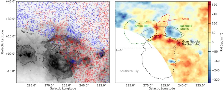
Figure2 (left) presents RMs from the Taylor et al. (2009) catalog over-plotted on the Ha image of the Gum Nebula. Although the lower left of the nebula is not covered by the NVSS, there are RM measurements toward the upper right with source densities varying between 1.2 and 6.6 deg−2 (Stil & Taylor 2007). It is easier to visualize RM features in the smoothed map created by Oppermann et al. (2012) mainly from the Taylor et al. (2009) catalog and plotted in Figure 2 (right). Using the Ha and radio continuum maps as a guide, we identify structures in the RM map likely associated with Galactic objects. The RM signature of the Gum Nebula is
clearly different from the background and matches the morphology of the excited hydrogen gas well. The distinctive upper arc of the nebula displays consistently positive RMs, which decrease in magnitude toward the geometric center, reminiscent of a limb-brightened shell. The net positive RM signal in the upper Gum Nebula implies a coherent magnetic field on scales of ∼260 pc, the projected diameter of the nebula at the adopted distance of d = 450 pc. The region along the Galactic mid-plane (∣ ∣ b 5) is highly confused, containing several HIIregions and SNRs (see Figure1), while the lower
part of the nebula also contains the IVS, which may be a separate foreground object. In contrast, the upper part of the Gum Nebula appears relatively free of obscuring objects and we focus on this region for the remainder of the paper. The gray wedge-shaped box in Figure 2 outlines the data selected for analysis. The selected region includes the upper arc of the nebula, the interior above b= 5 and a section of off-source RMs outside of the nebula’s border.
2.2.2. Isolating the RM signature of the Gum Nebula
Any analysis of the RM data relies on isolating the RM signature of the Gum Nebula from discrete regions of magneto-ionic material along the LOS (e.g., overlapping SNRs or HIIregions) and from the bulk of the Galaxy in the
background. We have identified three other sets of discrete Galactic objects toward the upper Gum Nebula that have Faraday rotation signatures in the Taylor et al. (2009) RM catalog. The Antlia SNR(McCullough et al. 2002) annotated in Figure 2) is adjacent to the nebula on the upper left. The edge of the SNR is traced by sources with RM values 10–15
-rad m 2more positive than their surroundings. This excess RM
signal is comparable to the formal error in the catalog (∼12
-rad m 2) and is negligible compared to RMs through the rim of
the Gum Nebula(∼300rad m-2). RMs through the interior of
the Antlia SNR are consistent with the background, except for a patch directly bordering the Gum Nebula, which is more negative than the large scale background by approximately −30.0rad m-2. This patch lies inside our selection box so we
Figure 2. Left: the RM catalog of Taylor et al. (2009) plotted over the aH map of the Gum Nebula(Finkbeiner2003). Red circles indicate positive RMs, while blue
indicate negative and their diameter is proportional to ∣RM . The solid∣ Hacontour at a level of 25 R defines the outline of the nebula. Right: prominent RM features are easier to visualize in the map produced by Oppermann et al.(2012) using the Taylor et al. (2009) catalog. Polygons and lines annotate significant features. We
subtract this offset from RMs inside the patch to correct the catalog. The second obvious feature in the data is a pair of shells discovered by Iacobelli et al. (2014) in 2.3 GHz radio continuum data, seen in polarization and lying to the upper-right of the Gum Nebula. The border of the shells seen in the radio data corresponds exactly to the morphology of a negative patch of RMs in Figure 2. We again correct the catalog by subtracting the median background offset(−77.2rad m-2) from
RMs inside the shell boundaries. The final feature of note is a “stalk” of positive RMs extending from the center of the upper arc to higher Galactic latitudes. The“stalk” has a counterpart in HIemission identified by Reynoso & Dubner (1997), lies
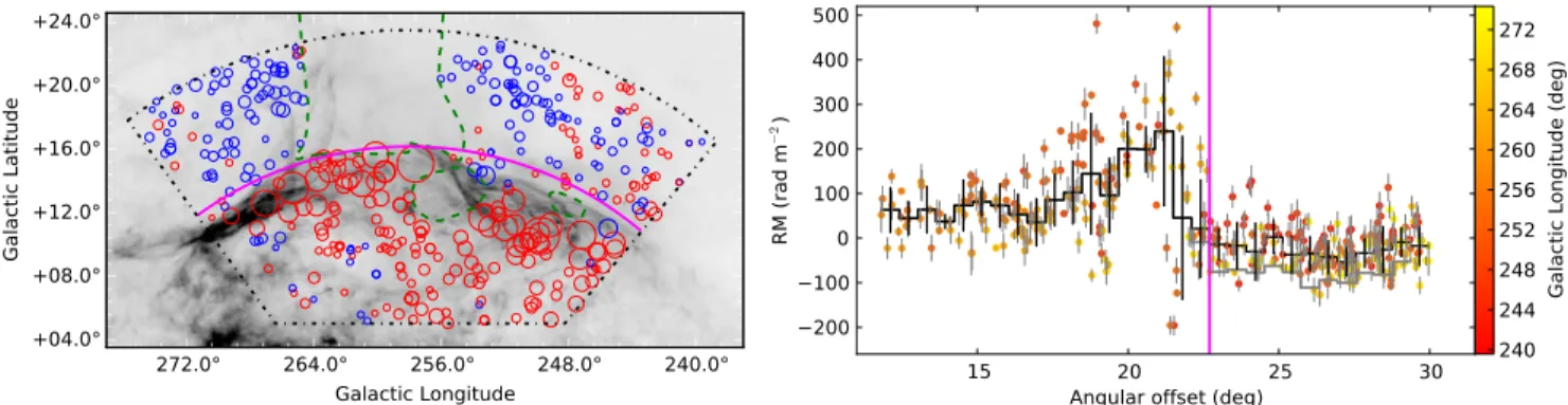
above a hole in the Ha image and is hypothesized by the authors to be a “blowout” in the shell wall leading to ionized gas streaming into the Galactic halo. Modeling and subtracting the signature of this feature is beyond the scope of this work, so we simply mask off the RM data within its boundary. Figure3 (left) presents the corrected RM catalog within the selection box, plotted over the Ha image. The azimuthally-averaged RM profile is shown in Figure3(right). The black histogram shows a version of the profile binned in 0◦. 6 increments.
Outside of the nebula border (offsets 22 ) the RMs are relatively constant but rise rapidly to a peak just inside the border. At smaller offsets the RM values fall slowly, approaching an interior level that is higher than the back-ground. The gray histogram, shows the same binned profile prior to correcting for discrete contaminating sources. Note that the RM data shown here have not yet been corrected for large-scale gradients due to diffuse thermal electrons distributed throughout the bulk of the Galaxy in the background.
The distribution of electrons within the Galaxy and the strength, and geometry, of the ordered Galactic magnetic field result in a unique pattern of RMs over the whole sky. In the all-sky RM map compiled by Oppermann et al. (2012) the dominant signal is quadrupolar in shape, with negative RMs above and positive below the Galactic mid-plane in the vicinity of the Gum Nebula. In recent years several authors have modelled the ordered Galactic field by combining data from extra-galactic RMs and radio-synchrotron emission (Sun et al. 2008; Jansson et al. 2009; Jaffe et al. 2010; Mao et al. 2010; Sun & Reich2010; van Eck et al.2011; Jansson & Farrar
2012), and explain the pattern as being due to the toroidal field in the halo. Within the Galactic disk the magnetic field and thermal electron density follow the spiral arms, increasing toward the mid-plane, leading to steep gradients in RM at low Galactic latitudes (Simard-Normandin & Kronberg 1980; Cordes & Lazio 2002; Gaensler et al. 2008). The sparse sampling of the Taylor et al.(2009) RM catalog and confusion toward the mid-plane mean that accurately removing the large-scale RM signal due to the Galaxy is challenging. We initially attempted tofit a 2D polynomial surface to the off-source RMs, but this proved to be highly unreliable in practice. Instead we consider two classes of potential RM backgrounds. In thefirst case we assume a simpleflat background at the median level of the selected RMs outside the boundary of the Gum Nebula: −26.4rad m-2. This assumption is the simplest correction
possible and consistent with the high-latitude RM data. However, we know that the volume-averaged electron density decays exponentially with height above the mid-plane(Cordes & Lazio 2002; Gaensler et al. 2008), thus the RMs must decrease correspondingly. Sun et al. (2008) and Jansson & Farrar(2012) have modelled the large scale RMs distribution of the Galaxy starting from the NE2001 electron density distribution and applying the scale height corrections of Gaensler et al. (2008). Both models have similar latitude profiles, illustrated for =l 258 in Figure 4(top). The bottom panel of Figure 4 shows the effect of subtracting each 2D model from the selected RM data-points. The resulting azimuthal profile is essentially the same for both models, but offset in RM as the models differ in their absolute calibration. Both models act to decrease the value of RMs toward the interior of the nebula. Neither model correctly predicts the absolute zero-level exterior to the Gum Nebula, likely because the best-fitting models are constrained over the whole sky and by other, sometimes contradictory, datasets. The authors also had limited knowledge of local contaminating objects. We adopt the RM models of Sun et al.(2008) and Jansson & Farrar (2012) as the best available estimates of the large-scale background variation in RM and apply offsets of −64.0 and −36.6rad m-2, respectively, so as to correct their calibration to
the zero-point exterior to the Gum Nebula. In our analysis of Figure 3. Left: positions of polarized extragalactic sources selected for analysis from the Taylor et al. (2009) catalog. Red and blue circles indicate positive and
negative RMs, respectively, and the radius of each circle is scaled to the absolute value of the RM. The green dashed lines enclose regions where sources have been excised from the sample because they likely probe a contaminating region, or are obvious outliers( s>3 ). Right: RMs plotted as function of angular offset from the center of the nebula. The formal uncertainties in the catalog are represented by vertical gray lines(scaled ´2 for clarity) and each point is color-coded for Galactic longitude. The solid black histogram represents a median-binned version of the plot, with bin-sizes of0 .6. The solid gray histogram illustrates the level of the RMs◦ exterior to the nebula before the discrete object correction was applied. Vertical black error-bars illustrate the1sscatter in each bin. The magenta line in both panels indicates the outer boundary of the nebula. In both panels the RMs are plotted assuming aflat background, i.e., no correction has been made for a large-scale RM gradient due to the Galaxy in the background(or foreground). The effect of subtracting different model backgrounds is illustrated in Figure4and discussed in Section2.2.1.
the RMs through the Gum Nebula we compare the results derived with each of these backgrounds separately.
2.3. 2.3 GHz Radio Continuum
Radio continuum at centimeter wavelengths traces gas emitting via both synchrotron and thermal processes. If information on the polarization state of the radiation is available, analysis of the Stokes Q and U parameters can constrain conditions in the gas along the LOS, e.g., depolarization due to afluctuating component of the magnetic field.
The S-PASS has imaged the entire southern sky (decl.< - 1 ) in polarization at a frequency of 2.3 GHz. The observations have been conducted with the Parkes Radio Telescope, NSW Australia, a 64 m telescope operated by CSIRO Astronomy and Space Science. A description of S-PASS observations and analysis is given in Carretti et al. (2010,2013b). Here we report a summary of the main details. The standard S-band receiver of the observatory(Galileo) was used with a system temperature Tsys=20 K, beam width FHWM = 8′.9 at 2300 MHz and a circular polarization front-end ideal for linear polarization measurements with a single-dish telescope. Data have been detected with the Digital Filter
Banks mark 3(DFB3) with full Stokes capabilities recording the two autocorrelation(RR and LL) and the complex cross-correlation products of the two circular polarizations(RR, LL, LR, RL*). Flux calibration was done with PKS B1934-638, secondary calibration with PKS B0407-658 and polarization calibration with PKS B0043-424. Data were binned in 8 MHz channels and, after RFI flagging, 23 sub-bands were used, covering the ranges 2176–2216 and 2256–2400 MHz, for an effective central frequency of 2307 MHz and bandwidth of 184 MHz.
The observing strategy is based on long azimuth scans taken toward the east and the west at the elevation of the south celestial pole at Parkes (EL = 33°) to realize absolute polarization calibration of the data. Final maps are convolved to a beam of FWHM= 10′.75 . Stokes I, Q, and U sensitivity is better than1.0 mJy beam-1per beam-sized pixel everywhere in
the covered area. Details of scanning strategy, map-making, andfinal maps obtained by binning all frequency channels are presented in Carretti et al.(2010) and E. Carretti et al. (2015, in preparation). The confusion limit is 6 mJy in Stokes I (Carretti et al. 2013a) and much lower in polarization (average polarization fraction in compact sources is lower than 2%, Tucci et al. 2004). The instrumental polarization leakage is 0.4% on-axis(Carretti et al.2010) and less than 1.5% off-axis. For diffuse emission, the latter is generally not important because of cancellation effects at scales larger than the beam (e.g., Carretti et al.2004; O’Dea et al.2007).
2.3.1. The Polarized Signature of the Gum Nebula
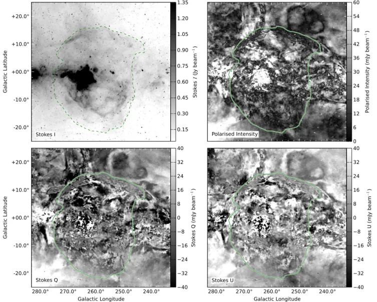
Figure5presents the 2.3 GHz radio-continuum image of the Gum Nebula in Stokes I, Q, U and polarized intensity P. The morphology of the nebula in total intensity is broadly similar to theHamap presented in Figure1, implying that the radio- and optical-emission are coming from the same gas. When viewed in P, Q, and U, the upper shell of the nebula is seen to depolarize background emission in a∼2° wide arc. This band of depolarization is set against the smooth Galactic back-ground, visible in the upper-right quadrant of the image, above
=
b 12 . At high latitudes the background is also depolarized by two thin shells(Iacobelli et al. 2014see Section2.2.1and Figure 2) and by the Antlia SNR in the upper-left quadrant. The shell of the Antlia SNR is similarly characterized by a band of depolarization that overlaps the Gum Nebula at
» +
l b
( , ) (268 , 13 ). The interiors of the Gum Nebula and Antlia SNR appear fractured, exhibiting patches of homo-geneous polarized intensity interspersed with depolarized “canals.” The Vela SNR at( , )l b =(267 , - 3 ) is the brightest object in thefield, (I and P), while the rest of the Galactic plane is seen as a mix of polarized foreground and depolarized background emission.
2.4. Pulsars
The ATNF Pulsar Catalogue(APC, Manchester et al.2005) collates the properties of more than 2300 rotation-powered pulsars and is continually revised as new discoveries are made. Of primary interest to us are the DMs, RMs, and distances to the pulsars. These parameters can be combined with EMs and a geometric model to derive the average electron density,filling factor, and magneticfield strength along the LOS.
We utilize version 1.49 of the APS, which lists 158 pulsars within a 30°radius of the kinematic center of the Gum Nebula Figure 4. Top: sample profiles at =l 259 from the models of Sun et al.
(2008) and Jansson & Farrar (2012) illustrating the predicted RM gradient
with Galactic latitude. Bottom: the light-gray histogram is the azimuthally averaged RM profile of the Gum Nebula uncorrected for discrete contaminating sources or large-scale RM background(also plotted in Figure3). The black
histogram is the equivalent with discrete corrections applied and a flat background of -26.4 rad m-2subtracted. The red(dashed) and green (dotted– dashed) histograms illustrate the effect of subtracting the 2D Sun et al. (2008)
and Jansson & Farrar(2012) RM models, respectively, from each point source
select from the Taylor et al.(2009) catalog. Note that the discrete corrections
have previously been applied. In both cases the large-scale gradient correction acts to decrease the RMs in the interior of the nebula relative to the exterior.
( =l 261 .0,◦ b = -2 .5; Woermann et al.◦ 2001). Of these we
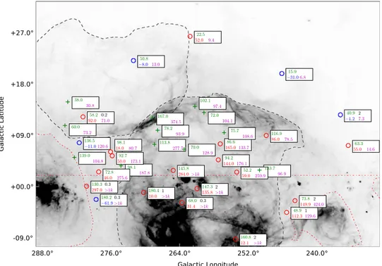
have chosen 35 for analysis, most of which lie within the upper Gum region. Figure 6and Table1 present this sample, which contains all pulsars aboveb= 2 and a handful below, chosen because they have accurately determined distances or lie on unconfused sight-lines adjacent to the Gum Nebula.
Accurate distances to pulsars are difficult to obtain: a handful of precise values have been calculated via annual parallaxes and these are limited to relatively nearby pulsars (<3 kpc). Kinematic distances accurate to ∼1 kpc can be derived for some pulsars associated with HIabsorption, while the distance
to pulsars located in globular clusters can be estimated to ∼15% reliability via analysis of color–magnitude diagrams. Most of the pulsars detected toward the Gum Nebula default to a distance derived from the dispersion measure. Such DM-distances are often highly inaccurate because they rely on a model of the Galactic free-electron distribution (Taylor & Cordes1993; Cordes & Lazio2002), which was itself created in part using the Taylor et al.(1993) pulsar catalog. Distances are particularly ill-determined toward the Gum Nebula, which was included in the Cordes & Lazio(2002) model as a pair of overlapping spheres of diameter 50 pc. It is not clear that this is
an improvement on the older Taylor & Cordes (1993) model which treated the nebula a simple Gaussian of FWHM 50 pc truncated at r = 130 pc. The Cordes & Lazio (2002) model does, however, account for the scatter broadening tsc, which
was measured by Mitra & Ramachandran(2001) for 40 pulsars between250 < <l 290 . They found that t scwas greater than
expected for a smooth Gaussian, implying a more inhomoge-neous distribution of ne. Based on the observed scattering they
concluded that pulsars in the vicinity of the Gum Nebula should be 2–3 times closer than predicted by Taylor & Cordes (1993). Within the area of the Gum Nebula only four pulsars have both DM measurements and accurate distances. The Vela pulsar(J0835-4510) is known to be at a distance of287-+17
19pc
(Dodson et al.2003), placing it just inside the front wall of the nebula. The remaining three (J0738-4042, J0837-4135 and J0908-4913) lie at distances greater than 1 kpc (see the bottom of Table1), behind the Gum Nebula.
3. ANALYSIS
Our analysis aims to answer the questions: What is the likely origin of the Gum Nebula? and What are the magnetic Figure 5. 2.3 GHz radio-continuum maps of the Gum Nebula from the S-PASS project. The data are calibrated in Janskys and may be converted to a main-beam brightness temperature scale in Kelvin by multiplying by 0.55. The border of the nebula traced by the green line is the same as in Figure2.
properties of the nebula and how do they affect ambient conditions in this part of the Galaxy? To address these questions we construct a simple model of the nebula as an ionized shell situated in the near field. We present the model below and explain the maximum-likelihood method used tofit the model to RMs on the sky. The model assumes a uniform density distribution plus a jump in ionization fraction from 0 to 100% within the shell of the Gum Nebula, which we derive from the Ha data and include as a prior in our fitting procedure. The resultingfits will be presented in Section4.
3.1. RMs as Magnetic Probes
Faraday rotation causes the polarization angle of a linearly polarized wave traversing a magnetized ionized medium to rotate by an angle D . The change in polarization angle isy given by
y l
D = RM 2 rad, (1)
where RM is the rotation measure in radians m−2. The observed RM depends on the LOS component of the magneticfield B∣∣
(in μG), the thermal electron density ne(incm-3) and the path
length dl(in pc) according to
ò
= n B dl -RM 0.81 e rad m . (2) src obs 2Note that the integral in Equation(2) is taken from the source of the polarized emission to the observer, so that a positive RM indicates an average magnetic field pointing toward the observer. If the ionized material along the LOS contains clumps of uniform ne threaded by the same B , then the∣∣
medium is characterized by a volume filling factor f.
Equation(2) becomes
= n B fL
-RM 0.81 e rad m ,2 (3)
where L is the total path length through the ionized medium and fL is known as the occupation length. L can generally be estimated from the geometry of the object under consideration (e.g., a slab, sphere or shell).
3.2. A Near-field Magnetic Bubble Model
Models of RMs through spherical ionized shells have recently been used to derive magnetic properties of Galactic SNRs and HIIregions, and to probe the magnitude and
orientation of the ordered Galactic magneticfield, e.g., Kothes & Brown(2009), Whiting et al. (2009), Harvey-Smith et al. (2011), and Savage et al. (2013). These phenomena ionise their surroundings and illuminate the ambient magnetic field via Faraday rotation. As they expand into the ISM they may also compress thefield, imprinting a specific signature on the RMs. Previous investigations have focused on distant objects (>1 kpc) whose small angular diameters (< 5 ) mean that they intercept fewer RM sight-lines compared to the nearby Gum Nebula. Because these bubbles lie in the far field, their RM profiles may be integrated in azimuth under the assumption of spherical symmetry. However, for a near-field bubble like the Gum Nebula, the sign and shape of the RM profile can vary with azimuth, depending on the orientation of the ordered magneticfield.
In a similar way to Whiting et al.(2009) and Savage et al. (2013), we model the Gum Nebula as a spherical ionized shell of radius R and thickness dr, threaded by a uniform, parallel magnetic field B0. We assume that the electron density ne is
constant within the shell and zero elsewhere (i.e., the Figure 6. Selection of pulsars with known DM values toward the Gum Nebula. All pulsars with > b 2 are shown alongside a selection of pulsars with accurate distances belowb= 2 . Red dotted–dashed lines outline confusing parts of the Galactic plane and pulsars in these regions have been omitted. “◦” symbols represent
pulsars with both DM and RM measurements, and“+” symbols pulsars with only DM measurements. Each pulsar is annotated with its DM inpc cm-3(top-left number, colored green), RM inrad m-2(bottom-left number, colored red or blue signifying positive or negative RM, respectively), independently determined distance in kpc, where known(top-right number, colored black) and EM inpc cm-6(bottom-right number, colored magenta).
background has been removed as in Section 2.1 and the electron density in the interior of the shell is negligible). The observer is located in the nearfield and the magnetic field lines make an angle Q to the plane of the sky in the direction of the bubble center. The tilt angle11of the magneticfield is assumed fixed along the y-axis, representing the Galactic plane, and the angle ζ describes the orientation of the sight-line to the yz-plane. The edge of the shell subtends an angular radius of f =sin (- R D)
outer 1 , where D is the distance from the observer
to the geometric center of the shell. A full description of the adopted geometry can be found in Appendix, including a detailed schematic.
If the shell is expanding supersonically into the ISM then the gas, and hence the magnetic field, will be compressed at the external boundary. If the expansion has slowed to sub-sonic speeds then the gas will simply move out of the way. To model the compression (or lack of) we assume the electron density behind the expansion front is given byne=X n0, where X is
the compression factor and n0 is the electron density in the
ambient medium. At each point on the sphere the component of the magnetic field tangent to the shell (B^) is amplified by X
while the normal component(Bn) is unaffected. The
contribu-tion to the observed magneticfield by one hemisphere is simply the vector sum ofX B and B^ nprojected along the LOS. The
measured RM is then proportional to the sum of the ingress(far hemisphere) and egress (near hemisphere) components. Equation (3) becomes a function of polar coordinate (ϕ,ζ), compression factor X, electron density ne, magnetic field
Table 1
Properties of Selected Pulsars Towards the Gum Nebula
(1) (2) (3) (4) (5) (6) (7)
Name l b DM RM D Notes
(deg.) (deg.) (cm−3pc) (rad m−2) (kpc)
Pulsars toward the upper Gum Nebula:
J0758-1528 234.464 07.224 63.327± 0.003 55± 7 3.72 Out J0818-3049 249.983 02.908 133.7± 0.2 L 4.17 Gum J0820-1350 235.890 12.595 40.938± 0.003 −1.2 ± 0.4 1.9† Out J0828-3417 253.965 02.561 52.2± 0.6 59± 3 0.5 Gum J0838-2621 248.807 08.981 116.9± 0.1 86± 13 4.6 Gum J0846-3533 257.190 04.710 94.16± 0.11 144± 8 1.4 Gum J0855-3331 256.847 07.517 86.635± 0.016 165± 10 1.2 Gum J0900-3144 256.162 09.486 75.702± 0.010 L 0.8 Gum J0904-4246 265.075 02.859 145.8± 0.5 284± 15 4.4 Gum J0908-1739 246.119 19.850 15.888± 0.003 −31 ± 4 0.6 Out J0912-3851 263.165 06.584 70± 1 L 0.6 Gum J0923-31 259.697 13.003 72± 20 L 1.0 Gum J0932-3217 261.277 14.069 102.1± 0.8 L 3.8 Gum J0934-4154 268.361 07.411 113.79± 0.16 L 3.2 Gum J0941-39 267.795 09.904 78.2± 2.7 L 1.3 Gum J0945-4833 274.199 03.674 98.1± 0.3 L 2.7 Out J0952-3839 268.702 12.033 167± 3 L 8.4 Gum,Ant J0959-4809 275.742 05.418 92.7± 1.2 50± 6 3.0 Out J1000-5149 278.107 02.603 72.8± 0.3 46± 9 2.3 Out J1003-4747 276.037 06.117 98.1± 1.2 18± 4 3.4 Out J1012-2337 262.131 26.377 22.51± 0.09 52± 9 1.3 Out J1032-5206 282.354 05.128 139± 4 L 4.3 Out J1034-3224 272.050 22.117 50.75± 0.08 −8 ± 1 4.7 Ant J1036-4926 281.518 07.727 136.529± 0.010 −11 ± 6 8.7 Out J1045-4509 280.851 12.254 58.166± 0.001 92± 1 0.23† Ant J1057-4754 284.007 10.739 60± 8 L 3.0 Ant J1105-43 283.511 14.886 38.000± 0.001 L 2.2 Ant
Pulsars below b= 2° with accurate distances:
J1001-5507 280.226 00.085 130.32± 0.17 297± 18 0.3† Out J0737-3039 B 245.236 −4.505 48.920± 0.005 112.3± 1.5 1.1† Out J0738-4042 254.194 −9.192 160.8± 0.7 12.1± 0.6 1.6† Gum J0742-2822 243.773 −2.444 73.782± 0.002 149.9± 0.1 2.0† Out J0835-4510 263.552 −2.787 67.99± 0.01 31.4± 0.1 0.28† Gum J0837-4135 260.904 −0.336 147.29± 0.07 135.8± 0.3 1.5† Gum J0908-4913 270.266 −1.019 180.37± 0.04 10.0± 1.6 1.0† Gum J0942-5552 278.571 −2.230 180.2± 0.5 −61.9 ± 0.2 0.3† Out
Notes. This table presents the properties of the pulsars displayed in Figure6. Pulsars marked with a † in column(6) have independent distance measurements; other entries default to the DM-derived distance. The code in column(7) notes whether the pulsar falls on a sightline toward the Gum Nebula (Gum), toward the Antlia SNR(Ant) or outside of the border of either object (Out).
11
The tilt angle is the angle the magneticfield makes to the Galactic disk at the position of the nebula.
strength B0and the angle of the magneticfield to the plane of the sky Q f z f = æ è çç çç Q ö ø ÷÷÷ ÷÷ æ è ççç öø÷÷÷ æ è çç ç ö ø ÷÷÷ ÷
-(
)
f B B X μ n L dr RM 0.81 , , , , G cm ( , ) pc . (4) e 0 3The model implicitly assumes that the same B∣∣ applies
everywhere along the half-chord between the outer surface and mid-plane of the shell (but different for ingress and egress). This assumption will only be realistic for a thin shell; a more sophisticated analysis is outside the scope of this paper. The model also assumes a constant value for the electron density within the shell and, because ne, Blos and f are degenerate in
Equation (3), the electron density and filling factor must be estimated from independent data, if possible(see Section 3.3, below).
Figure 7 presents a grid of near-field bubble models, illustrating how the RM observed on the sky changes as Q and X are varied. In the far-field case, the RM profile is spherically symmetric, i.e., constant withζ (the angle between
the profile sampling line and the Galactic plane, see Figure A1). However, in the near-field case the profile shape depends on bothζ and Q (the orientation of the ordered magnetic field vector). As Q increases from 0° (B0in the plane of the sky) to
90° (B0 pointing toward observer) the large scale distribution
of RMs changes from being anti-symmetric to symmetric around the central latitude axis. Increasing X leads to an overall increase in the magnitude of the RM and a large difference in RM between the center and inner-edge of the shell. The shape of the profile edge also becomes more rounded because of limb brightening, although this would be much more noticeable in far-field bubbles.
In Section 3.4, below, we present a maximum-likelihood method used to fit the model to RMs from the Taylor et al. (2009) catalog. We incorporate estimates of nefromHadata
as a prior, assuming Gaussian errors. 3.3. nefromHaData
From Equation(2) we see that neandB∣∣are degenerate and
cannot be determined individually from observations of RM Figure 7. Grid of models showing how changes in the angle of the magnetic field Q and the compression factor X affect the distribution of RMs across a simple ionized shell. The geometry of the model is described in theAppendix(see FigureA1.) and the parameters are set to: D = 450 pc, f =22 .7◦
outer , dr= 25.0 pc,
=
-ne 1.7 cm 3,B0=8.6 Gμ , and f= 0.5. Each model is presented in two panels: the upper panel presents a map of RM in offset Galactic coordinates and the lower panel displays radial RM profiles extracted over a range of angles Υ to the Galactic plane ( 0 ⩽¡⩽180).
alone. However, a separate observation of the EM provides an independent estimate of the electron density along the LOS. EM is related to nevia
ò
= ¥ n dl -EM e pc cm . (5) 0 2 6Assuming the same clumpy medium and geometry as presented in Section3.1this becomes
=n f L
-EM e2 pc cm ,6 (6)
with filling factor f and path length L as before. EM may be calculated directly from the intensity of theHa(3 -2) line via the equation of Reynolds(1988)
= æ è ççç öø÷÷÷ æ è çç ç ö ø ÷÷÷ ÷ -a T I K EM 2.75 10 K R cm pc, (7) e 4 0.9 H 6
where Teis the electron temperature in K,IHais the intensity of
the Ha emission in Rayleighs, and K=t (1-e-t) is a correction term to account for dust extinction between theHa emission and the observer(see Section2.1.1).
Most estimates of Te for the Gum Nebula within the
literature vary between 6500 and 11500 K. Electron tempera-tures derived by Reynolds(1976a) from a comparison of aH to[NII] linewidths are consistent with a uniform temperature of
11300 K throughout the nebula. However, Vidal (1979) determined the electron-temperature to be Te = 6500 K from
existing optical emission-line data. We adopt a uniform value of 8000 K for this analysis.
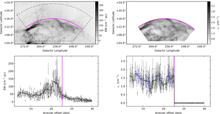
Figure8 (top-left) presents the EM map of the upper Gum region derived from the Finkbeiner (2003) Ha data using Equation (7). Azimuthally averaged EM values peak at
-220 pc cm 6 (see Figure 8, bottom-left), falling to
~80 pc cm-6 in the interior and 30 pc cm-6 outside the
nebula. Our values are largely consistent with those of previous authors. Reynolds(1976a) measured the EM via pointed aH spectral observation and found it varied from 100 pc cm-6
interior to the nebula to 240 pc cm-6 in the upper arc. Scans
across the region by Reynolds(1976a) at =l 240 determined the Galactic background to be <10 pc cm-6 rising to
-28 pc cm 6 at the mid-plane.
Assuming the geometry L( ,f dr) from the best-fit to our shell model(presented in Section4, below) and best-fit filling factor f = 0.3 we use Equations (6) and (A2) to derive the electron density ne inside the clumpy shell. The electron
density map and azimuthally averaged profile are presented in Figure8(right). The fitting procedure takes the value of neas a
prior(see Section3.4) altering the most likely shell geometry and filling factor f, requiring a new estimate of ne. To correct
for this inconsistency we re-calculated ne using the new
f
L( ,dr) and f, and iterated over thefitting loop until all values converged. The final electron density was determined to be
=
-ne 1.4 0.4 cm 3, which compares well with Reynolds (1976b) who found ne»1 cm-3 in the fainter parts of the nebula, assuming fixed physical parameters (fouter=18, D= 450 pc and15dr30 pc).
3.4. Maximum Likelihood Analysis
We use a Markov Chain Monte Carlo(MCMC) algorithm to fit the model shell to the RM data in the upper Gum region. The de-facto algorithm for performing MCMC fitting is the Metropolis–Hastings algorithm (Metropolis et al.1953; Hast-ings 1970), which randomly samples over parameter space, accepting or rejecting models based on their likelihood (i.e., the probability of the data given the model parameters). New positions with greater than previously are always accepted, while those with smaller are occasionally accepted. Our code Figure 8. Left: EM map and azimuthally averaged profile of the upper Gum region. The individual gray points in the bottom panel show the EM values at the positions of the RM samples while the black points with error bars show the azimuthal average and standard deviation in 0◦. 2 bins. Right: electron density map and azimuthal averaged profile derived assuming the best-fit parameters in Table2. The magenta line shows the edge of the shell model.
makes use of the efficient affine-invariant sampler (Goodman & Were 2010) implemented in the EMCEE12python module by Foreman-Mackey et al.(2013). EMCEE controls a number of parallel samplers, referred to as “walkers,” each of which corresponds to a vector of free parameters within the model. The walkers are initialized to a point in n-dimensional parameter space and are iteratively updated to map out the probability distribution. At each iteration the likelihood is calculated assuming Gaussian errors according to =e-c22
, where c2is the standard chi-squared goodness-of-fit statistic. If
priors with measured uncertainties exist for any model parameter, we incorporate them into the likelihood calculation by summing their chi-squared valuesc =c + åi c i
2 model 2 prior 2 .
Thefitter is started by generating 300 walkers initialized to random values of the free parameters. The MCMC code is initially run for 400“burn-in” iterations to allow the walkers to settle in a clump around the peak in likelihood space. The fitting routine is then run for 10,000 iterations to produce a well-sampled likelihood distribution. We determine the best fitting model from the mean of the marginalized posterior distribution for each free parameter. The1 uncertainties ares calculated as the fractional positions at1 -erf (1 )s =0.1572 and erf (1 )s =0.8427 on the normalized cumulative distribu-tion. Our results are presented in Section4.2
3.4.1. Scatter in RM as a Hyperparameter
The median measurement uncertainty on the selected RM data is s(RM)=12 rad m-2, considerably smaller than the
scatter evident in Figure 3 (right). The error-bars reflect only the uncertainty in the measurement and do not take into account systematic scatter, e.g., due tofluctuations in B or n∣∣ e
on scales much smaller than the sampling grid, or systematic errors in RM determination. We characterize this additional variation using a term d (RM) added in quadrature to the measurement uncertainty. This new scatter term is included in the model as a free parameter, however, it is treated slightly differently when calculating the likelihood function.
Lahav et al. (2000) and Hobson et al. (2002) present a formalism for performing joint analysis of cosmological datasets by introducing hyperparameter weighting terms, the values of which are determined directly from the statistical properties of the data. This approach is easily adapted to find the self-consistent uncertainties for data with ill-determined error-bars. Using Equations (29) and (30) of Hobson et al. (2002) we calculate a likelihood function using the modified chi-squared statistic
å
c s s = é ë ê ê ê -+ ù û ú ú ú(
)
(
)
π RM RM (RM) ln 2 (RM) , (8) i i i 2 i mod 2 tot, 2 tot, 2whereRMi-RMmodis the difference between the ith RM and
the model at that position. The second term inside the parentheses is required to correctly normalize the likelihood and the total uncertainty on the RMiis given by
s(RM)2tot,i=s(RM)i2 +exp 2 lnëé
(
d(RM)i)
ûù. (9)Here we solve forln ( (RM)) rather than directly for d (RM) sod as to enforce positivity in the scatter term (i.e., uncertainties cannot be negative).
4. RESULTS
4.1. General Comparison of Model and Data
Before presenting the results of the MCMC analysis, it is useful to visually compare the RM data shown in Figure3with the simple shell models illustrated in Figure 7. Two key discriminators stand out in the behavior of the models. First, the difference in RM between the interior and the peak of the shell (DRM, illustrated by the black line in Figure 7) is a strong function of the compression factor X, assuming other parameters are fixed. From Figure 3 (right) we see that the measured DRM in the profile of the northern Gum Nebula is ~350 rad m-2, restricting the compression factor to X4.
Models with higher values of X result in much greater DRM for all reasonable values of ne, f, B0, and Q. second, the
longitudinal RM gradient is directly related to the pitch angle of the magnetic field. This behavior is due to the close proximity of the nebula, so that sight-lines from opposite sides are not parallel and intersect a uniformfield at different angles. If the ordered magneticfield is directed along the plane of the sky at the nebula’s center (Q = 0 ), we would expect to measure equal positive and negative RMs on either side of the central longitude. For a magneticfield pointing directly toward (Q =90) or away (Q = - 90 ) from the Sun the RMs would display symmetric positive or negative patterns, respectively. We see mostly positive RMs toward the Gum Nebula, with a slight positive gradient toward lower Galactic longitudes (see Figure3). From an examination of the grid of models shown in Figure7, we can conservatively state that the ordered magnetic field is pointing toward the Sun at an angle Q 20 . This is because the negative peak in RMs at positive Galactic longitudes is absent from models with Q 20 , and from the Taylor et al.(2009) RMs. In Section4.2below we quantify these assertions usingfits to the data.
4.2. Fits to the Model Shell
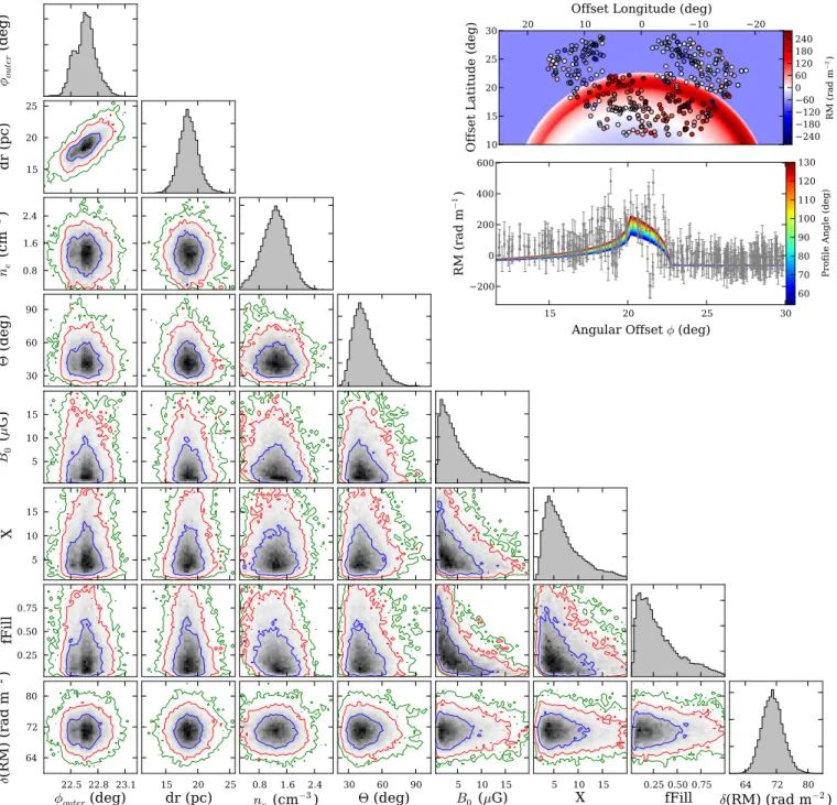
Here we present the results offitting the model described in Section3.2to a subset of the Taylor et al.(2009) RM catalog. The RM data included in the fit are outlined by the wedge-shaped box in Figure3 (left) and was selected to bracket the nebula above b > 5 (excluding the “stalk” region and a handful of negative outliers—see Section2.2.1). We fixed the center of the model to l b = ◦ - ◦
( , ) (258 .0, 6 .6) so that the circumference of the shell corresponds to the sharp outer edge seen in the Ha data (see Figure 1). The mean of the marginalized likelihood distribution is a good estimator of the best fitting value for each parameter; these are reported in Table2and described below.
We initially ran our MCMC fitting procedure assuming a flat, large-scale background of RM = -26.4 rad m
-bg 2 and
with all other parameters free, except distance, which wasfixed at D = 450 pc and electron density, for which a prior of
=
-ne 1.4 0.4 cm 3 was set (see Section 3.3). Likelihood distributions and plots of RM are presented in Figure9. The triangular matrix of confidence contour plots illustrates how the free parameters interrelate, while the histograms on the diagonal show the marginalized likelihood distributions for individual parameters. Of particular note are the distributions
12