Multi-view learning and data integration for omics data

(1)

UNIVERSITA’ DEGLI STUDI DI SALERNO DOTTORATO IN INFORMATICA E INGEGNERIA

DELL’INFORMAZIONE

CURRICULUM INFORMATICA

COORDINATORE: Ch.mo. Prof. Alfredo De Santis Ciclo XV N.S.

Multi-View Learning and Data Integration for omics Data

Relatori

Candidato

Ch.mo. Prof. Roberto Tagliaferri Angela Serra

Ch.mo. Prof. Dario Greco Matr. 8888100002

(2)

(3)

How to reach a goal? Without haste but without rest Goethe

(4)

(5)

Acknowledgements

During my PhD in the NeuRoNeLab I met wonderful friends whom I warmly thank: Luca, Paola, Massimo, thanks for the constant support, the countless

discussions and above all for the entertainment of the past three years.

A big thank you goes to the the special people I met in Helsinki: they never let me feel alone! Many thanks to Vittorio, Veer, Marit and Pia.

A special thank goes to my family who always support me.

I really do want to thank my mentors, Prof. Roberto Tagliaferri and Prof. Dario Greco, for the patient, the constant support and for the valuable advice

of the last three years.

Finally, the biggest thanks goes to Michele, without him I would not have come so far.

(6)

(7)

Abstract

In recent years, the advancement of high-throughput technologies, combined with the constant decrease of the data-storage costs, has led to the produc-tion of large amounts of data from diﬀerent experiments that characterise the same entities of interest. This information may relate to specific aspects of a phenotypic entity (e.g. Gene expression), or can include the comprehensive and parallel measurement of multiple molecular events (e.g., DNA modifications, RNA transcription and protein translation) in the same samples.

Exploiting such complex and rich data is needed in the frame of systems biology for building global models able to explain complex phenotypes. For example, the use of genome-wide data in cancer research, for the identification of groups of patients with similar molecular characteristics, has become a standard approach for applications in therapy-response, prognosis-prediction, and drug-development.ÂăMoreover, the integration of gene expression data regarding cell treatment by drugs, and information regarding chemical structure of the drugs allowed scientist to perform more accurate drug repositioning tasks.

Unfortunately, there is a big gap between the amount of information and the knowledge in which it is translated. Moreover, there is a huge need of computational methods able to integrate and analyse data to fill this gap.

Current researches in this area are following two diﬀerent integrative meth-ods: one uses the complementary information of diﬀerent measurements for the

(8)

study of complex phenotypes on the same samples (multi-view learning); the other tends to infer knowledge about the phenotype of interest by integrating and comparing the experiments relating to it with respect to those of differ-ent phenotypes already known through comparative methods (meta-analysis). Meta-analysis can be thought as an integrative study of previous results, usually performed aggregating the summary statistics from different studies. Due to its nature, meta-analysis usually involves homogeneous data. On the other hand, multi-view learning is a more flexible approach that considers the fusion of dif-ferent data sources to get more stable and reliable estimates. Based on the type of data and the stage of integration, new methodologies have been developed spanning a landscape of techniques comprising graph theory, machine learn-ing and statistics. Dependlearn-ing on the nature of the data and on the statistical problem to address, the integration of heterogeneous data can be performed at different levels: early, intermediate and late. Early integration consists in concatenating data from different views in a single feature space. Intermediate integration consists in transforming all the data sources in a common feature space before combining them. In the late integration methodologies, each view is analysed separately and the results are then combined.

The purpose of this thesis is twofold: the former objective is the definition of a data integration methodology for patient sub-typing (MVDA) and the latter is the development of a tool for phenotypic characterisation of nanomaterials (INSIdEnano). In this PhD thesis, I present the methodologies and the results of my research.

MVDA is a multi-view methodology that aims to discover new statistically relevant patient sub-classes. Identify patient subtypes of a specific diseases is a challenging task especially in the early diagnosis. This is a crucial point for the treatment, because not all the patients aﬀected by the same disease will have the same prognosis or need the same drug treatment. This problem is usually solved by using transcriptomic data to identify groups of patients that share the same gene patterns. The main idea underlying this research work is that to combine more omics data for the same patients to obtain a better characterisation of their disease profile. The proposed methodology is a late integration approach

(9)

based on clustering. It works by evaluating the patient clusters in each single view and then combining the clustering results of all the views by factorising the membership matrices in a late integration manner. The eﬀectiveness and the performance of our method was evaluated on six multi-view cancer datasets related to breast cancer, glioblastoma, prostate and ovarian cancer. The omics data used for the experiment are gene and miRNA expression, RNASeq and miRNASeq, Protein Expression and Copy Number Variation.

In all the cases, patient sub-classes with statistical significance were found, identifying novel sub-groups previously not emphasised in literature. The ex-periments were also conducted by using prior information, as a new view in the integration process, to obtain higher accuracy in patients’ classification. The method outperformed the single view clustering on all the datasets; moreover, it performs better when compared with other multi-view clustering algorithms and, unlike other existing methods, it can quantify the contribution of single views in the results. The method has also shown to be stable when perturbation is applied to the datasets by removing one patient at a time and evaluating the normalized mutual information between all the resulting clusterings. These ob-servations suggest that integration of prior information with genomic features in sub-typing analysis is an eﬀective strategy in identifying disease subgroups.

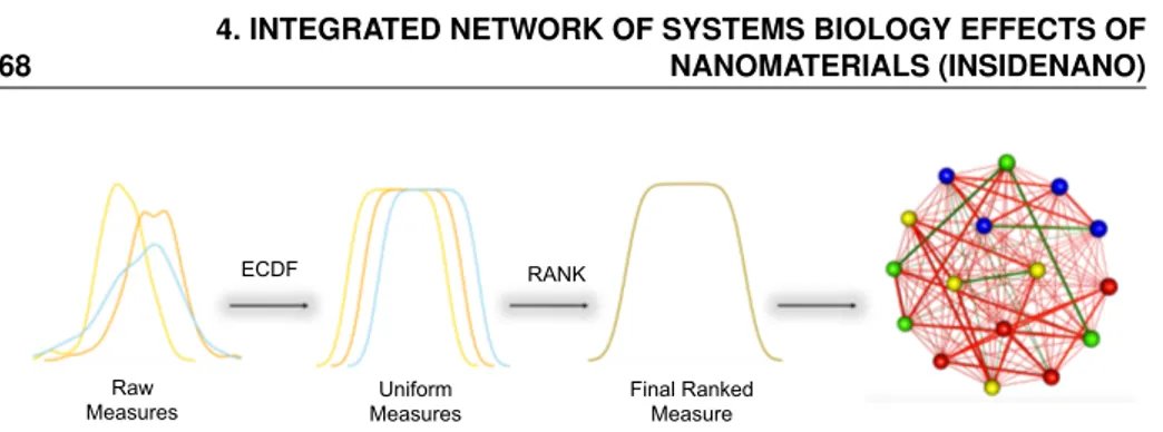
INSIdE nano (Integrated Network of Systems bIology Effects of nanomater-ials) is a novel tool for the systematic contextualisation of the effects of engin-eered nanomaterials (ENMs) in the biomedical context. In the recent years, omics technologies have been increasingly used to thoroughly characterise the ENMs molecular mode of action. It is possible to contextualise the molecu-lar effects of different types of perturbations by comparing their patterns of alterations. While this approach has been successfully used for drug reposition-ing, it is still missing to date a comprehensive contextualisation of the ENM mode of action. The idea behind the tool is to use analytical strategies to con-textualise or position the ENM with the respect to relevant phenotypes that have been studied in literature, (such as diseases, drug treatments, and other chemical exposures) by comparing their patterns of molecular alteration. This could greatly increase the knowledge on the ENM molecular effects and in turn

(10)

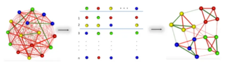
contribute to the definition of relevant pathways of toxicity as well as help in predicting the potential involvement of ENM in pathogenetic events or in novel therapeutic strategies. The main hypothesis is that suggestive patterns of similarity between sets of phenotypes could be an indication of a biological association to be further tested in toxicological or therapeutic frames. Based on the expression signature, associated to each phenotype, the strength of similar-ity between each pair of perturbations has been evaluated and used to build a large network of phenotypes. To ensure the usability of INSIdE nano, a robust and scalable computational infrastructure has been developed, to scan this large phenotypic network and a web-based eﬀective graphic user interface has been built. Particularly, INSIdE nano was scanned to search for clique sub-networks, quadruplet structures of heterogeneous nodes (a disease, a drug, a chemical and a nanomaterial) completely interconnected by strong patterns of similarity (or anti-similarity). The predictions have been evaluated for a set of known associations between diseases and drugs, based on drug indications in clinical practice, and between diseases and chemical, based on literature-based causal exposure evidence, and focused on the possible involvement of nanomaterials in the most robust cliques. The evaluation of INSIdE nano confirmed that it high-lights known disease-drug and disease-chemical connections. Moreover, disease similarities agree with the information based on their clinical features, as well as drugs and chemicals, mirroring their resemblance based on the chemical struc-ture. Altogether, the results suggest that INSIdE nano can also be successfully used to contextualise the molecular eﬀects of ENMs and infer their connections to other better studied phenotypes, speeding up their safety assessment as well as opening new perspectives concerning their usefulness in biomedicine.

(11)

4.2.4 Nanomaterials characterisation . . . 70 4.3 Results . . . 76 4.3.1 Network Description . . . 76 4.3.2 Nanomaterials Sub-network . . . 79 4.3.3 Nanomaterials-Drugs connections . . . 81 4.3.4 Nanomaterials-Disease connections . . . 81 4.3.5 Connections Validation . . . 81 4.3.6 Relevant cliques . . . 84 4.3.7 Use-case study . . . 85 4.4 Discussion . . . 89 5 Discussion 95 6 Conclusions and future work 101 Appendices 105 A Diﬀerentially expressed genes analysis 107 B Nanomaterials 111 C Complex Network Theory 117 C.0.1 Network properties . . . 120

(13)

List of Figures 147

(14)

(15)

List of Original Articles

Part of the work described in this thesis has been published in:

• A. Serra, M. Fratello, V. Fortino, G. Raiconi, R. Tagliaferri, and D. Greco, MVDA: a multi-view genomic data integration methodology, BMC bioin-formatics, vol. 16, no. 1, p. 261, 2015.

• Fratello, M., Serra, A., Fortino, V., Raiconi, G., Tagliaferri, R., and Greco, D. A multi-view genomic data simulator. BMC bioinformatics, vol 16, no,.1, 2015.

• A. Serra, D. Greco, and R. Tagliaferri (2015, July). Impact of diﬀerent metrics on multi-view clustering. In 2015 International Joint Conference on Neural Networks (IJCNN) (pp. 1-8). IEEE.

• A. Serra, M. Fratello, D. Greco, and R. Tagliaferri (2016, July). Data integration in genomics and systems biology. In 2016 World Congress on Computational Intelligence (WCCI). IEEE.

• A. Serra, I. Letunic, V. Fortino, B. Fadeel, R. Tagliaferri and D. Greco. Integrated network analysis links metal nanoparticles and neurodegener-ation. Manuscript Submitted

(16)

(17)

Chapter

1

Introduction

Cells are the basic structural, functional, and biological units of life and can be considered as the building block of all living beings [1].

They carry precise instructions in DNA concerning how they grow and func-tion. Complexity arose in the study of the cell phenotype, when it comes to study the dynamic aspects of the DNA at the level of genes, RNA transcripts, proteins, metabolites and their interactions.

In fact, the components of a biological system (for example, genes, proteins, metabolites and so on) function in networks and these networks interact with each other [2]. This gave birth to systems biology science whose main idea is that the molecular level of cells must be studied together organically and comprehensively, rather than separately. Since the objective of systems biology is to model the interactions in a system, the experimental techniques need to be system-wide and be as complete as possible. Therefore, there is a need to collect and to integrate diﬀerent kinds of data that are used to develop new approaches for the contextualisation of the behaviour of biological networks and to design and validate models [3–5].

Thanks to the technological advances in omics technologies and the decrease of storage costs, diﬀerent types of omics data have become available, among

(18)

them, there are gene expression, microRNA expression (miRNA), protein ex-pression, copy number variation (CNV) etc. Each of these experimental data provides potentially complementary information about the whole studied organ-ism.

Integrating these different sources is an important part of current systems biology research, since it is necessary to understand the whole biological system while the information coming from a single experiment is not sufficient. For ex-ample, the goal of functional genomics is to define the function of all the genes in the genome under a given condition. This is a difficult task that requires the integration from different experiments in order to be achieved [6]. Lanck-riet et al.[7] for example, aimed at classifying proteins as membrane proteins or not. They demonstrated that the integration of genomic data, amino acid se-quences and protein-protein interactions increase the classification performance compared to the use of only protein sequencing information.

Data integration methodologies arise in a wide range of clinical applications as well. Recently, new data integration techniques have been proposed to in-crease the clinical relevance of patients’ sub-classifications. Wasito et al. [8] proposed a kernel based integration method for lymphoma cancer sub-typing. They demonstrated that using the integration of DNA microarray and clinical data using Support Vector Machines (SVM) and Kernel Dimensionality Reduc-tion (KDR) improves the accuracy in the identificaReduc-tion of cancer subtypes. Sun et al. [9] employed multi-view bi-clustering to subtype cocaine users. They pro-posed a matrix decomposition approach that integrates already known genetic markers with clinical features to identify significant subtypes of the disease. Data integration also plays an important role in toxicogenomics, when research-ers want to undresearch-erstand the interaction between the genome and the environment to investigate the response of the genes to toxins and how they modify the gene expression function. Patel et al.[10] describes the contribution of diﬀerent data sources in advancing this field. The goals of data integration are to obtain higher precision, better accuracy, and greater statistical power than those provided by single datasets. Moreover, integration can be useful in validating results from diﬀerent datasets, under the assumption that if information from independent

(19)

data sources agrees, it is more likely that the information is more reliable than information from a single source. Unfortunately, there is a big gap between the amount of information and the knowledge in which it is translated. Even though many computational strategies have been developed to pre-process and analyse gene expression data, there is still a huge need of computational methods able to integrate and analyse gene expression data with other omics data.

1.1 Gene expression

The gene expression is the process by which the information contained in a gene is used to obtain a gene product that is often represented by proteins [11]. In a non-protein coding genes, such as the tRNA and small nuclear RNA (snRNA) genes, the final product is a functional RNA. It is worth mentioning that it is a common assumption to take the gene expression level as proportional to the amount of proteins translated. Indeed, several studies show that there exists a strong correlation between expression levels and protein abundance [12–14]. However, it is well known that there exist situations where the opposite is also true [15], [16]. In these cases, it is said that a post-transcriptional activity occurred.

This makes the role of gene expression of paramount importance in the study of the molecular profile of the cells. In fact, considering the existent relationship between gene expression and protein translation, the level of mRNA can provide indirectly knowledge on the state of the cell [17]. For example, by comparing the level of gene expression in healthy and diseased subjects, the molecular basis of the disease can be determined. Furthermore, by measuring the level of gene expression as a function of serial processes, the molecular changes over time (cell cycle), or the response to a specific drug or metabolite, can be identified.

Three are the options available for investigating the molecular dynamics of the cell, that give rise to three diﬀerent approaches: (1) proteomics, where the set of proteins in the cell are analysed, (2) transcriptomics, where the set of mRNA transcripts that lead to the production of proteins are analysed, (3) metabolomics, where the set of metabolites generated by the proteins are

(20)

ana-lysed. Research in proteomics and metabolomics has been ongoing for many years, but there is still a lack of standardised methodologies and poor reprodu-cibility of the experiments. On the other hand, the DNA microarray technology is a well-established tool for transcriptomic studies [18], [19]. DNA microarrays are not the only tool available to study the gene expression, new technologies such as RNA Sequencing, is becoming widely used for transcriptomic data ana-lysis.

1.2 1.2 High-throughput omics technology

Technological advancement allows simultaneous examination of thousands of genes with high-throughput techniques. Two of the major technologies used for transcriptomic analyses are DNA microarray and RNA sequencing. They both allow to measure gene expression but their protocol is substantially diﬀerent. Zhao et al.[20] demonstrate that RNA-Seq has some advantages with respect to DNA microarray. RNA-Seq technology has a higher capability in detecting low abundance transcripts. It also has a broader dynamic range than microar-ray, that allows to detect more diﬀerentially expressed genes with higher fold-changes. However, despite the benefits of RNA-Seq, microarrays are still widely used by researchers to conduct transcriptional profiling experiments. This is probably because microarrays are better known, data is easier to analyse and they are less expensive that RNA-Seq.

1.2.1 1.2.1 DNA microarrays

DNA microarrays have been proposed by Shena et al. in 1995 as a techno-logy able to simultaneously monitor the level of mRNA transcript for tens of thousands genes [21]. Even if the microarrays are used for a variety of diﬀerent purposes, such as comparative genomics hybridisation (CGH) [22] or CHIP-on-CHIP [23], their most popular application is still the large scale gene expression analysis. Microarrays have been also used to study several diseases, the cell cycle of various organisms as well as the regulation of many biological mechanisms.

(21)

Figu re 1.2.1: M ic roarr ay E xp erim en t: (a) Sp otte d m ic roarra y exp erim en tal se t-up . m RNA ex trac ts (tar-gets) from cells un der tw o distin ct ph ysiological con dition sare rev erse tran scrib ed to cDNA an d th en lab elled wi th di ﬀe re nt flu or es ce nt dy es e. g. Cy 3 an d Cy 5. E qu al am ou nt s of th e dy e-la be lle d ta rg et s ar e co m bi ne d an d ap pl ie d to a gl as s su bs tr at e on to wh ic h cD N A am pl ic on s or ol ig om er s (p ro be s) ar e im m ob ili se d. (b ) Sca nned ima ge of an A tl an ti c sa lmo n cD N A mi cr oa rr ay . F ig ue fr om T obi as et al .

(22)

Microarrays are small slides to which DNA molecules are bound. From the samples of each experimental condition the mRNA present in the cells is ex-tracted and manipulated (reverse transcription) to obtain complementary DNA (cDNA). At the same time, it is also labelled with fluorescent compounds (Cy3 green fluorescence, Cy5 red fluorescence) to mark each class of sample. The cDNA sequences hybridised with complementary sequences are positioned on the microarray spots. The slide is then scanned with a laser light at diﬀerent wavelengths. For each spot the fluorescence intensity is recorded. The spots that respond to green light correspond to genes expressed only in first exper-imental condition, whereas spots responding to red light correspond to genes expressed only in the second experimental condition; finally, the spots respond-ing to both lights (i.e. yieldrespond-ing a yellow fluorescence) indicate genes expressed in both experimental conditions. The intensity of the expression level is given by the intensity average of the corresponding spots in the image. This process is illustrated schematically in Figure 1.2.1.The expression values derived from measurements made on the microarray are noisy and need to be pre-processed, corrected with respect to the background [24] and normalised [25], [26].

1.2.2 1.2.2 RNA Sequencing

Another technology used to quantify gene expression is based on next-generation sequencing (NGS) to reveal the presence and quantity of RNA in a biological sample at a given moment in time [27], [28]. Classical DNA sequencing tech-niques aims to identify the order of the four bases in a DNA strand. NGS, also called high-throughput sequencing technologies, allows to parallelize the sequencing process, producing thousands or millions of sequences concurrently [29], [30]. The main diﬀerences between Microarray technology and RNA-Seq is that with the Microarray only a limited number of genes, those bound on the spots, can be studied. On the other hand, with RNA-Seq methodology a scanning of the whole genome is performed, allowing to investigate both known transcripts and exploring new ones. Therefore, RNA-seq is ideal for discovery-based experiments [28]. For example, 454-discovery-based RNA-Seq has been used to sequence the transcriptome of the Glanville fritillary butterfly [31]. Moreover,

(23)

RNA-Seq has very low background signal, in fact, DNA sequences can been mapped to unique regions of the genome [28].

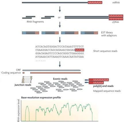
The standard work-flow of an RNA-seq analysis is composed of three steps (see Figure 1.2.2): (1) the RNAs in the sample of interest are fragmented and reverse-transcribed to create a library of complementary DNAs fragments (cD-NAs). (2) The obtained cDNAs are then amplified (i.e. duplicated millions of times [32]) and subjected to NGS to obtain short sequences. (3) The short reads generated can then be mapped on a reference genome. The number of reads aligned to each gene are called counts and gives a digital measure of gene expression levels in the investigated sample [33].

There are multiple methods for computing counts. The most used method considers the total number of reads overlapping the exons (i.e. the portion of a gene that is transcribed by RNA polymerase during the transcription process) of a gene [34].

However, it can happen that a fraction of reads maps outside the boundaries of known exons [35]. Thus, alternatively, the whole length of a gene can be considered, also counting reads from introns (i.e. non-coding region of the genes that are transcribed by RNA polymerase). The ’Union-Intersection gene’ model considers the union of the exonic bases that do not overlap with the exons of other genes [36].

After computing the counting, two kinds of biases have to be removed [37– 39]. The former to be taken into account is the sequencing depth of a sample, defined as the total number of sequenced or mapped reads. For two given RNA-seq experiments A and B, if A generates twice the number of reads than the experiment B, it is likely that the counts from experiment A will be doubled. To solve this problem, a common practise is to scale counts in each experiment by the sequencing depth estimated for the sample [40].

The latter is related to gene length [36, 41]; in fact, the expected number of reads mapped into a gene is proportional to both the abundance and length of the isoforms transcribed from that gene. Indeed, longer genes produce more reads than shorter ones. To reduce this bias, Mortazavi et al. [42] proposed to summarise the reads with the "Reads Per Kilobase of exon model per Million

(24)

systems have already been applied for this purpose. The Helicos Biosciences

tSMS system has not yet been used for published RNA-Seq studies, but is also appropriate and has the added advantage of avoiding amplification of target cDNA. Following sequencing, the resulting reads are either aligned to a reference genome or reference transcripts, or assembled de novo without the genomic sequence

example, 454-based RNA-Seq has been used to sequence the transcriptome of the Glanville fritillary butterfly27_{. This} makes RNA-Seq particularly attractive for non-model organisms with genomic sequences that are yet to be determined. RNA-Seq can reveal the precise location of transcription boundaries, to a single-base resolution. Furthermore, 30-bp short reads from RNA-Seq give information

signal because DNA sequences can been unambiguously mapped to unique regions of the genome. RNA-Seq does not have an upper limit for quantifica-tion, which correlates with the number of sequences obtained. Consequently, it has a large dynamic range of expres-sion levels over which transcripts can be detected: a greater than 9,000-fold range was estimated in a study that analysed 16 million mapped reads in Saccharomyces cerevisiae18_{, and a range spanning five} orders of magnitude was estimated for 40 million mouse sequence reads20_{. By} contrast, DNA microarrays lack sensitivity for genes expressed either at low or very high levels and therefore have a much smaller dynamic range (one-hundredfold to a few-hundredfold) (FIG. 2). RNA-Seq

has also been shown to be highly accurate for quantifying expression levels, as deter-mined using quantitative PCR _(qPCR)18_and

spike-in RNA_{controls of known}

concentra-tion20_{. The results of RNA-Seq also show} high levels of reproducibility, for both technical and biological replicates18,22_. Finally, because there are no cloning steps, and with the Helicos technology there is no amplification step, RNA-Seq requires less RNA sample.

Taking all of these advantages into account, RNA-Seq is the first sequencing-based method that allows the entire transcriptome to be surveyed in a very high-throughput and quantitative man-ner. This method offers both single-base resolution for annotation and ‘digital’ gene expression levels at the genome scale, often at a much lower cost than either tiling arrays or large-scale Sanger EST sequencing.

Challenges for RNA-Seq

Library construction. The ideal method

for transcriptomics should be able to directly identify and quantify all RNAs, small or large. Although there are only a few steps in RNA-Seq (FIG. 1)_{, it does}

involve several manipulation stages dur-ing the production of cDNA libraries,

Nature Reviews | Genetics

Base-resolution expression profile Exonic reads or Nucleotide position RNA expr ession le ve l

Coding sequenceORF

Junction reads

Mapped sequence reads Short sequence reads

EST library with adaptors

RNA fragments cDNA

mRNA AAAAAAAA AAAAAAAA TTTTTTTT ATCACAGTGGGACTCCATAAATTTTTCT CGAAGGACCAGCAGAAACGAGAGAAAAA GGACAGAGTCCCCAGCGGGCTGAAGGGG ATGAAACATTAAAGTCAAACAATATGAA ... ...AAAAAA ...AAAAAAAAA

poly(A) end reads

Figure 1 | A typical RNA-Seq experiment. Briefly, long RNAs are first converted into a library of cDNA fragments through either RNA fragmentation or DNA fragmentation (see main text). Sequencing adaptors (blue) are subsequently added to each cDNA fragment and a short sequence is obtained from each cDNA using high-throughput sequencing technology. The resulting sequence reads are aligned with the reference genome or transcriptome, and classified as three types: exonic reads, junction reads and poly(A) end-reads. These three types are used to generate a base-resolution expression profile for each gene, as illustrated at the bottom; a yeast ORF with one intron is shown.

P E R S P E C T I V E S

Figure 1.2.2: A typical RNA-seq experiment. Briefly, long RNAs are first converted into a library of cDNA fragments through either RNA fragmenta-tion or DNA fragmentafragmenta-tion (see main text). Sequencing adaptors (blue) are subsequently added to each cDNA fragment and a short sequence is obtained from each cDNA using high-throughput sequencing technology. The resulting sequence reads are aligned with the reference genome or transcriptome, and classified as three types: exonic reads, junction reads and poly(A) end-reads. These three types are used to generate a base-resolution expression profile for each gene, as illustrated at the bottom; a yeast ORF with one intron is shown. Figure and Legend from [28].

(25)

mapped reads" (RPKM) measure, that is computed by dividing the number of reads aligned to a gene exon, by the total number of reads mapped and by the sum of exonic bases.

microRNA expression

MicroRNAs (miRNAs) are small (approximately 18-24 nucleotides) non-coding RNA molecules of single-stranded DNA, which bind to mRNAs and regulate protein expression, either promoting degradation of the mRNA target and/or by blocking translation [43, 44], or alternatively by increasing translation [45]. miRNA are mainly active in the regulation of gene expression at the transcrip-tional and post-transcriptranscrip-tional levels. They have been found to be involved in numerous cell functions such as proliferation, diﬀerentiation, death [46, 47]. The aberrant expression of miRNAs has been implicated in the onset of many diseases [48, 49] and they can be used for therapeutic purposes [50]. Profiles of miRNAs in various types of tumors have been shown to contain potential diagnostic and prognostic information [51]. The study of mirna expression is slightly more complicated than the study of gene expression. Several technical variables must be taken into account in problems related to microRNA isolation, the stability of stored miRNA samples and microRNAs degradation [52]. As for gene expression, microRNA expression can be quantified by hybridization on microarrays, slides or chips with probes to hundreds or thousands of miRNA targets, so that relative levels of miRNAs can be determined in diﬀerent samples [53]. microRNAs can be both discovered and profiled by high-throughput se-quencing methods (microRNA sese-quencing) [54].

1.3 Biological Databases

Given the large number of omics data produced, there have been many eﬀorts made to collect the results of the experiments and make them available to the research community. In fact, many are the biological available online databases, which contain the experimental data (either in raw form that pre-processed) and the knowledge produced by such experiment (i.e. the connection between

(26)

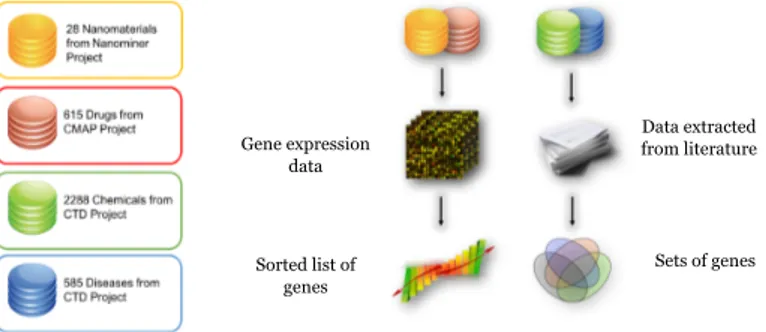
the gene and disease). Examples of database that provide experimental data are The Cancer Genome Atlas (TCGA - [55]), the Gene Expression Omnibus (GEO [56]) databases, the Connectivity Map (CMAP - [57]) and the NanoMiner ([58] ) databases.

The TCGA is a public repository that collects samples related to more that 30 diﬀerent tumours. It makes available the clinical information of the samples, metadata regarding technicalities of the experiments, histopathology images and molecular diﬀerent information such as mRNA/miRNA expression, protein expression, copy number, etc. GEO is a public repository that collect array and sequence-based data coming from the scientific community and makes them available to the public. It provides tool to help the user to query and download experiments and curated gene expression profiles. CMAP is a collection of transcriptional expression data from human cells treated with drugs. The main goal of the project was to discover functional connections between drugs, genes and diseases through the transitory feature of common gene-expression changes. NanoMiner database contains in-vitro transcriptomic data on human samples exposed to nanoparticles.

On the other side, some examples of database collecting knowledge extracted from the experiments are the Comparative Toxicogenomics Database (CTD [59] ), the Medicaton Indication dataset (MEDI [60]) and the Molecular Signature Database (MSigDB [61]).

CTD is a robust, publicly available database that aims to advance under-standing about how environmental exposures aﬀect human health. It provides manually curated information about chemicalâĂŞgene/protein interactions, chem-icalâĂŞdisease and geneâĂŞdisease relationships. These data are integrated with functional and pathway data to aid in development of hypotheses about the mechanisms underlying environmentally influenced diseases. MEDI is an ensemble resource of electronic medical record (EMR) data. It contains inform-ation related to the drugs that have been prescribed to treat certain diseases. The MSigDB is a collection of annotated gene sets, that are useful for the GSEA analysis or to evaluate the biological meaning of clusters of genes. All these data can be used to perform integrative analysis both with multi-view and

(27)

meta-analysis techniques.

1.4 Data Integration

Data integration (or data fusion) methodologies integrate multiple datasets in order to increase the accuracy, to reduce the noise and to extract more accurate information from multi modal datasets by finding correlation across them. Fig-ure 1.4.1 reports a classification of the integration methodologies based on the statistical problem, the type of analysis to be performed, on the type of data to be integrated and on the integration stage as described in [62].

Type of Analysis

The analysis to be performed is somehow limited by the type of data involved in the experiment and by the desired level of integration. Analyses can be di-vided into two categories: meta-analysis and integrative analysis. Meta-analysis can be thought as an integrative study of previous results, usually performed aggregating the summary statistics from diﬀerent studies [63, 64]. Due to its nature, meta-analysis can only be performed as a step of late integration in-volving homogeneous data. On the other hand, integrative analysis is a more flexible approach that considers the fusion of diﬀerent data sources to get more stable and reliable estimates. Based on the type of data and on the stage of integration, new methodologies have been developed spanning a landscape of techniques comprising graph theory, machine learning and statistics.

Type of Data

Data integration methodologies in systems biology can be divided into two cat-egories based on the type of data: integration of homogeneous or heterogeneous data types. Usually biological data are thought to be homogeneous if they assay the same molecular level, for gene or protein expression, copy number variation, and so on. On the other hand if data is derived from two or more diﬀerent molecular levels they are considered to be heterogeneous. Integration of this

(28)

F ig ur e 1.4 .1 : D at a In te gr at io n T ax on om y

(29)

kind of data poses some issues: first, the data can have different structure, for example they can be sequences, graphs, continuous or discrete numerical values. Moreover, data coming from different sources is subject to different noise levels depending on the platform and on the technologies used to generate data. The integration process must include a step, called batch effect removal where the noise and the random or systematic errors between the different views become comparable [65].

Integration Stage

Depending on the nature of data and on the statistical problem to address, the integration of heterogeneous data can be performed at diﬀerent levels: early, intermediate and late. Early integration consists in concatenating data from diﬀerent views in a single feature space, without changing the general format and nature of data. Early integration is usually performed in order to create a bigger pool of features by multiple experiments. The main disadvantage of early integration methodologies is given by the need to search for a suitable distance function. In fact, by concatenating views, the data dimensionality considerably increases, consequently decreasing the performance of the classical similarity measures [66]. Intermediate integration consists in transforming all the data sources in a common feature space before combining them. In classification problems, every view can be transformed in a similarity matrix that will be combined in order to obtain better results. In the late integration methodolo-gies each view is analysed separately and the results are then combined. Late integration methodologies have some advantages over early integration tech-niques: (1) the user can choose the best algorithm to apply to each view based on the data; (2) the analysis on each view can be executed in parallel.

(30)

F ig ur e 1.4 .2 : D at a in te gr at io n sta ge pr op os ed by P av lid is et al [6 7]. Th ey pr op os ed an SV M ke rn el fu nc tio n in or de r to in te gr at e m icr oa rra y da ta . In ea rly in te gr at io n m eth od olo gie s SV M s ar e tra in ed wi th a ke rn el ob ta in ed fro m th e co nc at en at io n of all th e vie ws in th e da ta se t (a ). In in te rm ed ia te in te gr at io n, fir st a ke rn el is ob ta in ed fo r ea ch vie w, an d th en th e co m bin ed ke rn el is us ed to tra in th e SV M (b ). In th e la te in te gration me th od ology a sin gle SVM is train ed on a sin gle ke rn el for eac h vie w an d th en th e fin al re su lts are com bin ed (c).

(31)

Chapter

2

Aim of the study

The aim of this work is to provide new data integration tools to help the scientific community. Particularly, I have focused on two main objectives:

• The definition of a methodology that integrates multiple omics feature sets to find statistical relevant patient subtypes.

• The development of a tool for phenotypic characterisation of nanomateri-als mode-of-action with respect to human diseases, drugs treatments and chemicals exposures.

(32)

(33)

Chapter

3

Multi View Learning for Patient

Subtyping

In this chapter the multi-view genomic data integration methodology (MVDA) is described. MVDA is a clustering based methodology proposed to identify patient sub-types by combining multiple high-throughput molecular profiling data. It is a late integration approach where the views are integrated at the levels of the results of each single view clustering iterations. By using MVDA, patient sub-classes with statistical significance were retrieved, identifying novel sub-groups previously not emphasised in literature. The content of this chapter is published in [68].

3.1 Introduction

Many diseases - for example, cancer, neuropsychiatric, and autoimmune dis-orders - are diﬃcult to treat because of the remarkable degree of variation among aﬀected individuals [69]. Trying to solve this problem a new discipline emerged, called precision medicine or personalized medicine [70]. It tries to individualize

(34)

the practice of medicine by considering individual variability in genes, lifestyle and environment with the goal of predicting disease progression and transitions between disease stages, and targeting the most appropriate medical treatments [71].

A central role in precision medicine is played by patients subtyping, that is the task of identifying subpopulations of similar patients that can lead to more accurate diagnostic and treatment strategies Identify disease subtypes can help not only the science of medicine, but also the practice. In fact, from a clinical point of view, refining the prognosis for similar individuals can reduce the uncer-tainty in the expected outcome of a treatment on the individual. Traditionally, disease subtyping research has been conducted as a by-product of clinical exper-ience, wherein a clinician noticed the presence of patterns or groups of outlier patients and performed a more thorough (retrospective or prospective) study to confirm their existence.

In the last decade, the advent of high-throughput biotechnologies has provided the means for measuring diﬀerences between individuals at the cellular and mo-lecular levels. One of the main goals driving the analyses of high-throughput molecular data is the unbiased biomedical discovery of disease subtypes via unsu-pervised techniques. Using statistical and machine learning approaches such as non-negative matrix factorization, hierarchical clustering, and probabilistic lat-ent factor analysis [72], [73], researchers have idlat-entified subgroups of individuals based on similar gene expression levels. For example, the analysis of multivari-ate gene expression signatures was successfully applied to discriminmultivari-ate between disease subtypes, such as recurrent and non-recurrent cancer types or tumour progression stages [74]. To improve the model accuracy for patient stratifica-tion, in addition to gene expression, other omics data type can be used, such as miRNA (microRNA) expression, methylation or copy number alterations. For example, somatic copy number alterations provide good biomarkers for cancer subtype classification [75]. Data integration approaches to eﬃciently identify subtypes among existing samples has recently gained attention. The main idea is to identify groups of samples that share relevant molecular characteristics. Strategies of data integration of multiple omics data types poses several

(35)

compu-tational challenges, as they deal with data having generally a small number of samples and diﬀerent pre-processing strategies for each data source. Moreover, they must cope with redundant data as well as the retrieval of the most relevant information contained in the diﬀerent data sources. When the integrated data are high dimensional and heterogeneous, defining a coherent metric for cluster-ing becomes increascluster-ingly challengcluster-ing. A number of data integration approaches for patients subgroups discovery were recently proposed, based on supervised classification, unsupervised clustering or bi-clustering [76–79]. Moreover, multi-view clustering methodologies have been intensively used also if in few cases on omics data

3.2 Materials and Methods

3.2.1 Clustering

Clustering is an unsupervised learning technique, able to extract structures from data without any previous knowledge on their distribution. It is one of the main exploratory techniques in data mining and it is used to group a set of objects in such a way that objects in the same group (called a cluster) are more similar to each other than to those in other clusters.

Clustering have been widely applied in bioinformatics. Two of the main problems addressed by clustering are: (1) identify groups of genes that share the same pattern across diﬀerent samples [80]; (2) identify groups of samples with similar expression profiles [81]. The number of diﬀerent clustering tech-niques proposed in literature is huge. Two of the most common approaches are hierarchical clustering or partitive clustering [82].

The former methods start having each object in diﬀerent clusters and then they, iteratively, join couple of similar clusters until they reach a stop criterion. This kind of methodology creates a hierarchy of the clusters that is called dendrogram. The crucial point in hierarchical clustering is the evaluation of the measure between two clusters. Diﬀerent measures have been proposed such as: the single-linkage, where the distance between two clusters is defined as the

(36)

minimum distance between each couple of points between the two clusters; the complete linkage computes the distance between two clusters as the maximum distance between each couple of points. In the average linkage the distance between two clusters is computed as the mean of the distances between all the couples of objects between the two clusters. Ward’s minimum variance linkage aims to minimise the total within-cluster variance. All these methods produce a hierarchy of the samples, in order to clustyer data, this hierarchy must be cut at a certain height that is arbitrary chosen by the user. To solve this problem the Pvclust [83] algorithm have been proposed. It is a hierarchical clustering algorithm that applies a multi-scale bootstrap re-sampling procedure to the dataset, to compute a p-value that is used to cut the tree to obtain clusters that are statistically supported by data.

The latter methods, conversely, start from a group of initial points, called centroids, that represent the clusters and in an iterative manner, assign each sample in the dataset to a centroid and if necessary update the centroids. The whole process aims to minimise an objective function, and the algorithm runs until convergence or until a stop criterion is reached. Examples of this kind of algorithms are Kmeans [84], Partitional Around Medoids (PAM) [85] and SOM [86].

Given a set of observations (x1, x2, . . . , xn), where each observation is a

d-dimensional real vector, k-means clustering [84] aims to partition the n obser-vations into k( n) sets S = S1, S2, . . . , Sk so as to minimise the within-cluster

sum of squares (WCSS) In other words, its objective is to find:

arg min x K X i=1 X x2Si ||x µi||2 (3.2.1)

where µi is the mean of the points in Si. The optimal solution is obtained

iterating two diﬀerent steps: the former in which each point is assigned to the nearest centroid, and the latter in which the centroids are updated to minimise the equation 3.2.1.

Partitional Around Medoids [85] is a clustering algorithm related to the K-means algorithm and the medoids shift algorithm. Both the K-means and

(37)

K-medoids algorithms are partitional (breaking the dataset up into groups) and both attempt to minimise the distance between points assigned to a cluster and a point designated as the centre of that cluster. Contrary to the K-means algorithm, K-medoids chooses data points as centres (medoids or exemplars) and works with an arbitrary matrix of distances between data points;

SOM [86], is a type of artificial neural network (ANN) that is trained using unsupervised learning to produce a low dimensional (typically two-dimensional), discretised representation of the input space, called a map. Self-organising maps are diﬀerent from other artificial neural networks in the sense that, during the training phase, they use a neighbourhood function to preserve the topological properties of the input space. A self-organizing map consists of components called nodes or neurons. Associated with each node there are a weight vector of the same dimension of the input data vectors (prototype), and a position in the map space. The usual arrangement of nodes is a two-dimensional regular spacing in a hexagonal or rectangular grid. The self-organising map describes a mapping from a higher-dimensional input space to a lower-dimensional map space. The procedure for placing a vector from input space onto the map is to find the node with the closest (smallest distance metric) weight vector to the data space vector. This makes SOMs also useful for obtaining low-dimensional views of high-dimensional data, akin to multidimensional scaling.

The SOM is trained iteratively. At each training step, a sample vector x is randomly chosen from the input data set. Distances between x and all the prototype vectors are computed. The best-matching unit (BMU), which is denoted here by b, is the map unit with prototype closest to x

||x mb|| = mini||x mi||. (3.2.2)

Next, the prototype vectors are updated. The BMU and its topological neighbours are moved closer to the input vector in the input space. These two iterations are repeated until convergence. At the end, all the points assigned to the same neuron in the SOM will be allocated in the same cluster.

A clustering algorithm diﬀerent from these two families is the spectral clus-tering [87]. The general approach to spectral clusclus-tering starts from a similarity

(38)

matrix, then computes the relevant eigenvector of its Laplacian. In the space of these eigenvectors, a classical clustering algorithm, such as K-means is executed. Traditional state-of-the-art spectral methods [87] aim to minimise RatioCut [88], by solving the following optimisation problem:

min

Q2Rn⇥cT race(Q

T_L+_Q) _s.t.QT_{Q = I} _(3.2.3)

where Q = Y (YT_{Y )} 1/2 _{is a scaled partition matrix, L}+ _{denotes the}

nor-malised Laplacian matrix L+_{= I} _D 1/2_{W D} 1/2 _{given the similarity matrix}

W.

When performing a clustering analysis, the first problem is to choose the algorithm that best fits the problem. There are many different clustering al-gorithms and the application of each one will usually produce different results. Moreover the results of the algorithms strongly depend on the input parameters (such as the number of clusters). Without additional evaluation, it is difficult to determine which solutions are better. To solve this problem some indexes have been proposed to asses the clustering solutions [89]. Usually algorithms are executed with different parameters and then solutions that reach the best values of the evaluation indexes are selected.

3.2.2 Multi-View Clustering

The main difference between traditional and multi-view clustering is that the former takes multiple views as a flat set of variables without taking into account differences among different views, while the latter exploits the information from multiple views and takes the differences among the views into consideration in order to produce a more accurate and robust data partitioning. Multi-view clustering has been widely applied in machine learning by using different variants of existing single view clustering methodologies [90–95]. Moreover, it has been widely applied to integrate different genome-wide measurements in order to identify cancer-subtypes [76–78, 93, 96].

Chen et al. [91] proposed the early integration method Two-level variable Weighting k-means (TW-kmeans) clustering for multi-view data. This method

(39)

extends the classical k-means algorithm by incorporating the weights of the views and of the variables into the distance function that identifies clusters of objects. The algorithm is able to identify the set of k clusters, the important views and the relevant variables for each view. The authors evaluated the per-formance of the TW-k-means algorithm for classification of real life data, by testing it on three data sets from UCI Machine Learning Repository.

The algorithm proposed by Long et al. [94] exploits the intuition that the optimal clustering is the consensus clustering shared across as many views as possible. This can be reformulated as an optimisation problem where the op-timal clustering is the closest to all the single view clusterings under a certain distance or dissimilarity measure. Clusterings are again represented as mem-bership matrices. Formally the model can be described as follow: given a set of clustering membership matrices M = [M1, . . . , Mh]2 Rn⇥l+ , a positive integer k

and a set of non-negative weights {wiR+}mi=1, the optimal clustering membership

matrix B 2 Rn⇥k

+ and the optimal mapping matrices P = [P1, . . . , Ph]2 Rk⇥l+

are given by the minimisation:

min

B,P h

X

i=1

wiGI(M(i)||BP(i))

s. t. P 0

B 0, B1 = 1

(3.2.4)

where GI(M||BP ) is the generalised Kullback-Leibler divergence such that

GI(X_{||Y ) =}X ij (logXijlog Xij Yij Xij+ Yij)

subject to the constraint that both P and B must be non-negative and that each row of B must sum to one. The method has been evaluated on both synthetic and two real data sets: the former is a web page advertisement data-set and the latter is a newspaper dataset. They executed the multi-view clustering algorithm ten times on each dataset by imposing the number of clusters equal to the number of real classes and evaluated the final multi-view clustering with

(40)

respect to the real class labels with the Normalised Mutual Information. They demonstrated that the integration methodology gives better results compared to those obtained with the use of single view separately and the experiments showed that the algorithm eﬃciently learns robust consensus patterns from multiple view data with diﬀerent levels of noise.

Green et al. [95] proposed a meta-analysis technique for multi-view cluster-ing in a late integration manner. The main idea is to use the matrix factorisation approach to combine clustering results on each single view expressed in form of membership matrices.The method first transposes all the membership matrices and stacks them vertically in order to obtain the cluster matrix X in R l×n where l is the total number of clusters in C and n is the number of samples. Then, it iteratively finds the best approximation of X such that X ⇡ P H and P 0, H 0 by measuring the error with the Frobenius norm and the update rules proposed by Lee et al. [97]. The results of the factorisation are two matrices,

P _{2 R}{l⇥k} _{that projects the clusters into a new set of k meta-clusters and}

H _{2 R}{k⇥n} _{whose columns can be viewed as the membership of the original}

objects in the new set of meta-clusters. Starting from the values of P , a matrix

T _{2 R}{v⇥k} _{is computed, with v being the number of views. T}

hf indicates the

contribution of the view Vhto the fth meta-cluster. The method has been

eval-uated on both synthetic and real-world document datasets. In both settings it produced more informative clusterings with respect to the single view clustering counterparts. It turned out that the method can eﬀectively take advantage of cases when a variety of diﬀerent clusterings are available for each view and in fact out-performed popular ensemble clustering algorithms.

Yang et al. [98] proposed a biclustering algorithm, based on matrix factor-isation, for module detection in multi-view genomic data sets. Their method, called iNMF is a modification of the jSNF algorithm [99]. Both methods are able to factorise multi-view datasets but, while jSNF considers all the views as having the same eﬀect on the resulting factorisation, iNMF allows each view to bring its own contribute to the factorisation process. The method was tested on a real ovarian cancer dataset coming from TCGA. The dataset was composed of three views: DNA methylation, gene expression and miRNA expression. The

(41)

method was able to detect multi-modal modules and sample clusters that agree with the ones already in the literature.

iCluster [96] uses a joint latent-variable model to identify the grouping struc-ture in multi omics data. This method simultaneously achieves data integration and dimension reduction, by reporting all the views to a common space, that has a number of latent variables significantly smaller than the originals ones, and clustering patients in that space. The optimal space is identified in an optimiz-ation process that uses the EM algorithm and a Lasso model that penalises the norm of the coefficient vectors and continuously shrinks the coefficients associ-ated with non-informative genes toward zero, to ensure the data sparseness. The method was tested by simultaneously clustering gene expression, genome-wide DNA copy number and methylation data derived from the TCGA Glioblastoma Multiforme samples. The authors compared their method with a naive integ-ration obtained by concatenating the views and applying PCA. Their results showed that iCluster had better capability to stratify patients by integrating different omics views.

On the other hand, SNF [93] is an intermediate integration network fusion methodology able to integrate multiple genomic data (e.g., mRNA expression, DNA methylation and microRNA expression data) to identify relevant patients’ subtypes. The method first constructs a patients’ similarity network for each view. Then, it iteratively updates the network with the information coming from other networks in order to make them more similar at each step. At the end, this iterative process converged to a final fused network. The authors tested the method combining mRNA expression, microRNA expression and DNA methyl-ation from five cancer data sets. They showed that the similarity networks of each view have diﬀerent characteristics related to patients similarity while the fused network gives a clearer picture of the patients’ clusters. They compared the proposed methodology with iClust and the clustering on concatenated views. Results were evaluated with the silhouette score for clustering coherence, Cox log-rank test p-value for survival analysis for each subtype and the running time of the algorithms. SNF outperformed single view data analysis and they were able to identify cancer subtypes validated by survival analysis.

(42)

MEREDITH [77] is an intermediate late integration approach methodology to discover cancer sub-typing by integrating multiple omics feature sets. This methodology is composed of several steps comprising data normalisation, data integration, clustering and validation. Since, it is a gene centred method, as a first step, all the features in the diﬀerent views are mapped to the corres-ponding genes. Then, a PCA analysis is performed to reduce the dimension-ality of each view. The first 50 PCs per dataset with the highest eigenvalues are retained and then scaled and concatenated to construct a single integrated dataset. A mapping into a two-dimensional space is performed by means of the t-distributed stochastic neighbourhood embedding. The clustering analysis and survival analysis is performed. The method was tested on more that 4000 patients coming from the The Cancer Genome Atlas (TCGA)across 19 cancer-types and four views: gene expression, DNA-methylation, copy-number vari-ation and microRNA expression. The performed DBSCAN clustering was able to identify 18 clusters significantly over-represented by a cancer type (p < 0.001). MEREDITH was then able to identify known cancer types and subtypes. This results suggest that data integration methodologies could enable novel insight in patients characterization.

The proposed methodology for the analysis of multi-view biological datasets takes in input n matrices Mi2 RFi⇥P for i = 1, . . . , n where Fiis the number of

features (genes, miRNAs, CNV, methylation, clinical information, etc.) and P is the number of patients and a vector cl of classes labels, and yields a multi-view partitioning G =Sk

i=1Giof patients. The multi-view integration methods also

return a matrix C where ci,jis the contribution of view i to the final multi-view

cluster j.

The approach consists of four main steps as shown in Figures 3.2.1 and 3.2.2: (a) Prototype Extraction; (b) Prototype ranking; (c) Single view clustering; (d) late integration.

In the prototype extraction step, the features with low variance across the samples were eliminated. Therefore, the data were clustered with respect to the patients and the cluster centroids were selected as the prototype patterns. The centroid of each cluster was selected as the most correlated element with

(43)

Figu re 3.2.1: Firs t tw o ste ps of th e M VD A m eth od ology . A dim en sion alit y re du ction is pe rf orm ed by cl us te ri ng th e fe at ur es . A pr ot ot yp e is ex tr ac te d fo r ea ch cl us te r to re pr es en t it in th e fo llo wi ng st ep s (a ) Th e pr ot ot yp es ar e ra nk ed by th e pa ti en t cl as s se pa ra bi lit y an d th e m os t si gn ifi ca nt on es ar e se le ct ed (b ).

(44)

Figu re 3.2.2: Las t tw o ste ps of th e M VD A m eth od ology . Sin gle vie w clu ste rin g m eth od s are ap plie d in eac h view to gr oup pat ien ts and obt ai n mem ber shi p mat rices (c) . A lat e in tegr at ion appr oac h is ut ilised to in te grate clu ste rin g re su lts (d ).

(45)

respect to the other elements in that cluster. Diﬀerent clustering algorithms were used such as Hierarchical clustering with Ward’s method [100], Pvclust [83], Kmeans [84], PAM [85] and SOM [86]. See section 3.2.1 for more detail on these clustering algorithms.

The idea is to evaluate several popular clustering techniques and compare their behaviour on the diﬀerent views with respect to the hierarchical method that is the standard algorithm used to cluster genes. Cluster analysis is a complex and interactive process and results change based on its parameters [101]. Therefore, each algorithm was executed for diﬀerent values of K. For each algorithm and for each K, clustering performance was evaluated according to the following evaluation function:

V AL = 1 4 ✓_{IC + 1} 2 + 1 IE + 1 2 + (1 S) + CG ◆

where IC is the complete diameter measure, representing the average sample correlation of the less similar objects in the same cluster; EC is the complete linkage measure, representing the average sample correlation of the less similar objects for each pair of clusters; S is the singleton factor and CG is the compres-sion gain. The evaluation function was defined in order to obtain the output value normalised between 0 and 1. The complete diameter and the complete linkage measures were calculated with the R "clv" package [102]. The number of singleton was normalised in a range (0,1) in order to be comparable with the correlation measure. It was defined as S = N/(K−1). The compression gain was defined as CG = 1−(K/Nelem), where K is the number of clusters and N is the number of elements to be clustered. Each clustering algorithm was executed on n diﬀerent values of K and the corresponding results were evaluated with the function V AL. Values close to 1 indicate a clustering with similar objects in the clusters, weakly linked clusters, with few singletons and with a good compres-sion rate. A numeric score was then assigned to each K value by considering the average values of the VAL function compiled over the clustering results obtained with the diﬀerent algorithms. Then, the K showing the highest score was chosen and subsequently used to identify the best clustering algorithms having the first

(46)

two highest scores with respect to the selected k value.

The V AL index is a validity index measure such as the Dunn Index or David Bouldin Index [103]. It measures the compactness and separation of the clusters. A "good" clustering should have two characteristics: compactness and separation. A clustering is compact when the members of each cluster are as close to each other as possible. The compactness is measured by the IC value. The separation is therefore measured by the EC value, the less the correlations between two diﬀerent clusters the more they are separated.

More detail on the computational procedure followed to fine-tuned the k-values for the cluster analysis can be found in the article [68].

In the prototype ranking, further dimensional reduction by feature selection was performed. Feature ranking was computed by means of the CAT-score [104] and the Mean Decreasing Accuracy index calculated by Random Forests [105]. For each rank, the cumulative sum of the ranking score was computed and four diﬀerent cuts based on the cumulative values were taken. Cuts considered all the features needed to maintain 60 %, 70 %, 80 % and 90 % of the cumulative value. These diﬀerent groups of features were used to cluster patients in each single view (single view clustering step), with the same single view clustering algorithms used in the first step. The number of clusters K was considered as the number of classes. For each clustering, the error was calculated as the dispersion obtained in the confusion matrix between class labels and clustering assignments. The clustering algorithm that reached the minimum error for each view was then selected.

These clustering results were used as the input to the late integration step to obtain the final muti-view meta clusters. The integration was performed by using both Greene [95] and Long [94] approaches. Once the multi-view clusters were obtained, a subclass was assigned to each one. For each cluster, the number of objects of each class was calculated and the class with more representative patterns was assigned as the cluster label. Then, a p-value was calculated in order to verify the statistical significance of the subclass by the Fisher’s exact test [106]. Experiments were performed in two ways: the former uses all the prototypes for classification; the latter uses only the most relevant

(47)

ones for class separability. Each one of these approaches were performed both in unsupervised and semi-supervised manners, respectively. The semi-supervised approach consists of giving a priori information as input to the techniques of late integration via a membership matrix of patients with the exact information of their classes. This information is combined with the membership of the patients compared to the single view clustering and integrated in meta-clusters. This can be a useful approach mainly when the data set is composed of unbalanced or under represented classes.

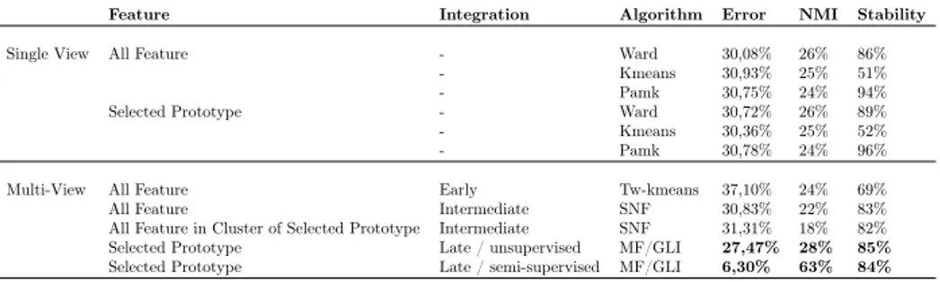
MVDA was compared with classical single view clustering algorithms (Kmeans, Hierarchical and Pam), early (TW-Kmeans) and intermediate (SNF) integration approaches. For each method clustering impurity, normalised mutual informa-tion (NMI) and cluster stability were evaluated. Cluster impurity was defined as the number of patients in the cluster whose label diﬀers from that of the cluster. Given two clustering solutions the NMI was computed as the mutual information between the two clustering normalised by the cluster entropies. The NMI was computed between clustering results and real patient classifications.

The stability of the system was tested by giving diﬀerent inputs to the al-gorithm and comparing the results. In order to perform the highest number of comparison, and avoid to have unbalanced patient classes, the dataset was altered with leave-one-out technique.

A test was run on the first step to generate a stability index for the proto-types of the obtained clusters. Then, the steps 2, 3 and 4 were evaluated jointly to assess the stability of the selected features and to evaluate the robustness of the multi-view clustering results. Furthermore, a borda-count method [107] was performed to find the final list of features selected over the leave-one-out experiments for the integration step. At the end of this process, N diﬀerent clustering assignments were obtained, one for each removed patient. An mat-rix was created, where M(i, j) was the normalised mutual information (NMI) between the clustering obtained removing patient i and the clustering obtained removing patient j. Then the mean of the matrix was calculated, indicating the stability measure of the method.

(48)

data types, such as the Cancer Genome Atlas (TCGA) data sets ([55]). The comparison experiments suggest that MVDA outperforms other existing integ-ration methods, such as Tw-Kmeans and SNF.

3.3 Dataset collection and preparation

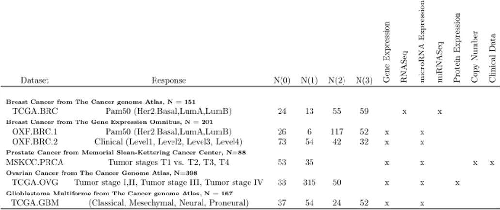
The experiments were performed on six genomic datasets (see Table 3.1). They were downloaded from The Cancer Genome Atlas (TCGA) ([55]), Memoral Sloan-Kettering Cancer Center ([108]) and from NCBI GEO ([56]) (See Table 3.1). Since all the data downloaded were already pre-process ed, only the batch eﬀect was removed by the comBat method in the R âĂĲsvaâĂİ package [109]. For the dataset TCGA.BRC, the RNASeq and miRNASeq (level 3) data re-lated to breast cancer patients, with invasive tumors, were downloaded from the TCGA repository (https://tcga-data.nci.nih.gov/tcga/ - Breast invasive carcinoma [BRCA]). Patients were subsequently divided into four classes (Her2, Basal, LumA, LumB), using PAM50 classifier [110, 111].

mRNA (GSE22219) and microRNA (GSE22220) expression data related to breast cancer patients, from a study performed at Oxford University [112], were downloaded from Gene Expression Omnibus Dataset [56]. Patients were divided into four classes (Her2, Basal, LumA, LumB), using PAM50 classifier [110, 111]. This dataset was namend OXF.BRC.1. The same patients were then classified into four classes (Level1, Level2, Level3, Level4) using clinical data also retrieved from the same source. This dataset was namend OXF.BRC.2.

For the TCGA.GBM dataset, the gene and miRNA expression (level 3) data related to patients aﬀected by Glioblastoma, were downloaded from the TCGA repository (https://tcga-data.nci.nih.gov/tcga/ - Glioblastoma multiforme [GBM ]). Also, clinical data was retrieved. The patients were divided info four classes: Classical, Mesechymal, Neural and Proneural as described in [113].

For the dataset TCGA.OVG the gene expression, protein expression, and miRNA expression (level 3) data related to patients aﬀected by ovarian cancer, were downloaded from the TCGA repository (https://tcga-data.nci.nih. gov/tcga/ - Ovarian serous cystadenocarcinoma [OV ]). Clinical data were

(49)

Table 3.1: Datasets: Description of the datasets used in this study. "N" is the number of subjects for each dataset. N(i) is the number of samples in the i-th class. An x denotes if that view (column) is available for a specific dataset (row). Dataset Response N(0) N(1) N(2) N(3) Gene E xp re ss ion RNAS eq micr oRNA Expr ession miRNASeq Prot ei n Ex pr essi on Co py N um be r Cl in ic al D at a

Breast Cancer from The Cancer genome Atlas, N = 151

TCGA.BRC Pam50 (Her2,Basal,LumA,LumB) 24 13 55 59 x x

Breast Cancer from The Gene Expression Omnibus, N = 201

OXF.BRC.1 Pam50 (Her2,Basal,LumA,LumB) 26 6 117 52 x x

OXF.BRC.2 Clinical (Level1, Level2, Level3, Level4) 73 54 42 32 x x

Prostate Cancer from Memorial Sloan-Kettering Cancer Center, N=88

MSKCC.PRCA Tumor stages T1 vs. T2, T3, T4 53 35 x x x x

Ovarian Cancer from The Cancer Genome Atlas, N=398

TCGA.OVG Tumor stage I,II, Tumor stage III, Tumor stage IV 33 315 50 x x x

Glioblastoma Multiforme from The Cancer genome Atlas, N = 167

TCGA.GBM (Classical, Mesechymal, Neural, Proneural) 37 54 24 52 x x

downloaded to classify patients in three categories. In particular patients were classified by clinical stage: first class: stage IA, IB, IC, IIA, IIB and IIC, second class: IIIA, IIIB and IIIC, third class Stage IV.

For the dataset MSKCC.PRCA, the gene expression, microRNA expression, copy number variation (CNV) and clinical data related to patients aﬀected by prostate cancer, were downloaded from the Memorial Sloan Kettering Cancer Center ([114]). Clinical data were downloaded to classify patients in three cat-egories. Patients were classified in two classes by using clinical data by the tumour stage: class one is Tumour Stage I and class two is Tumour Stage II, III and IV. Classification of patient was done according to a previous study performed on the same dataset [115].