Modelling flow and heat transfer in helically coiled pipes - Part 2: Direct numerical simulations for laminar, transitional and weacly turbulent flow in the case of zero pitch

(1)

(2)

CIRTEN

C

ONSORZIO

I

NTERUNIVERSITARIO

PER LA

R

ICERCA

T

ECNOLOGICA

N

UCLEARE

UNIVERSITA’ DI PALERMO

DIPARTIMENTO DI INGEGNERIA NUCLEARE

Modelling flow and heat transfer in

helically coiled pipes

Part 2: Direct numerical simulations for laminar, transitional

and weakly turbulent flow in the case of zero pitch

Modellazione numerica del campo di moto

e dello scambio termico in condotti elicoidali

Parte 2: Simulazioni numeriche dirette per moto laminare, transizionale e

debolmente turbolento nel caso di passo nullo

F. Castiglia, P. Chiovaro, M. Ciofalo, M. Di Liberto, P.A. Di Maio,

I. Di Piazza, M. Giardina, F. Mascari, G. Morana, G. Vella

CIRTEN-UNIPA RL-1205/2010

Palermo, Novembre 2009

Lavoro svolto in esecuzione delle linee progettuali LP2 punto G dell’AdP ENEA MSE del 21/06/07, Tema 5.2.5.8 – “Nuovo Nucleare da Fissione”

(3)

ABSTRACT

The present report comes further to a previous one on the subject (A. Caronia et al., Modellazione numerica del campo di moto e dello scambio termico in condotti elicoidali, Rapporto CIRTEN-UNIPA RL-1202/2008), which should be regarded as Part 1 of a broader study.

Here, time-dependent numerical simulation results are presented for the flow with heat transfer of a constant property fluid with Pr=1 in toroidal pipes. Two curvatures (=0.1 and 0.3) were considered. The friction Reynolds number was made to vary between 220 and 525, yielding flow Reynolds numbers (based on bulk velocity and pipe diameter) between 4531 and 14710 and Dean numbers between 1625 and 7219. A finite volume method was used and the full torus was discretized by computational grids having 3.3106_{nodes for the higher curvature (}__{=0.3) and 11.4}₁₀6 _{nodes for} the smaller one (=0.1). According to the Reynolds number, different flow regimes were predicted. For Re<5200, the flow was stationary for both curvatures. For 5200Re6000, the flow was periodic for=0.3 and quasi-periodic for=0.1; spectra exhibited isolated frequencies associated with the existence of travelling waves which were also identified and characterized by flow visualization. Proper Orthogonal Decomposition (POD) was applied to the results in order to identify different modes. For Re>6000, both curvatures exhibited chaotic flow which became fully turbulent, with a continuous frequency spectrum, for Re>10 000. In the whole range of conditions examined, heat transfer results were in good agreement with the Reynolds analogy.

Although the conditions explored in the present study are different from those expected for helical pipe steam generators under normal operation, the present results are a useful complement to more industrially-oriented studies like those reported in the previous report. A full understanding of a component’s behaviour under its prescribed nominal operating conditions may come only from considering the influence of parameters such as flow rate, curvature and torsion in a sufficiently broad interval. Moreover, at the higher end of the present Reynolds number range (Re14,000) the present simulations aim to set high-quality reference results against which to validate RANS simulations, while in the transitional range (Re4,000 - 6,000) they are aimed at clarifying the mechanisms by which low-Reynolds number, steady and laminar solutions lose stability and chaotic (turbulent) flow is eventually established, thus assisting the designers to interpret experimental friction and heat transfer results such as those reported by Cioncolini and Santini19_{. The issue of the applicability of} zero-pitch results to the case of finite pitch (helical coils) will be better discussed in the Conclusions.

(5)

NOMENCLATURE

a tube radius [m]

ai(t) time-dependent coefficients of POD

c coil radius [m]; dimensionless celerity, cˆ/

u

ˆ

_av

ˆ

c celerity of a travelling wave [m s1_] De Dean number,

Re 

f Darcy-Weisbach friction coefficient; dimensionless frequency,

f

ˆ

/

f

ˆ

₀

ˆ

f

frequency [s1_]

0

ˆ

f

frequency scale, (De) / (2a2_{) [s}1_]

K dimensionless turbulent kinetic energy, Kˆ/

u

ˆ

_av2

ˆ

K turbulent kinetic energy [m2_s2_]

k* _{number of wavelengths contained in the torus}

KDean Dean parameter,

(

p a

s2 7

) /(8



2 4

c

) (1/ 2)Re



4



L dimensionless wavelength, Lˆ/a

ˆ

L wavelength [m]

N number of control volumes (grid cells) Nu Nusselt number,

q a

w

2  

(

T T

b w

)

Pr Prandtl number,cp/

ps driving pressure gradient [Pa m1]

qw wall heat flux [W m-2]

Re bulk Reynolds number, uav2a/

Re friction Reynolds number,

u

ˆ

a/

ˆ

r radial coordinate from cross section centre [m]

r dimensionless radial coordinate from cross section centre, rˆ/a

ˆ

_p

(6)

rp dimensionless radial coordinate from torus centre,

ˆ

p

r

/a ˆ T temperature [K] T dimensionless temperature,

(

T T

ˆ ˆ ˆ ˆ



w

) /(

T

b



T

w

)

us dimensionless axial velocity,

u

ˆ

_s/

u

ˆ

_av

ˆ

_s

u

axial velocity [m s1_]

ˆ

_av

u

average velocity [m s1_]

ˆ

u

_ friction velocity [m s-1_]

z dimensionless vertical coordinate

Greek symbols

i eigenvalues of POD

i cumulative fraction of variance in POD,



_i

/





_i

 dimensionless curvature, a/c

 dissipation of turbulence energy [m2 _s3_] K Kolmogorov length scale [m]

 kinematic viscosity [m2_s-1_]

 density [kg m-3_]

 thermal conductivity [W m-1_K-1_]

 azimuthal angle [radians]

w wall shear stress [Pa]

0 equilibrium wall shear stress , (a/2)ps[Pa]

i(x,y) spatial eigenfunctions of POD

0 reference angular velocity,

2 

u

ˆ

_av



/

a

[s1]

2 dimensionless angular celerity of a travelling wave,



ˆ

₂/0

2

ˆ

_

(7)

2,fl dimensionless angular velocity of the fluid,



ˆ

_{2 ,}__fl/0

2 ,

ˆ

__fl



angular velocity of the fluid [s1_]

Subscripts

AX axial av average b bulk

cr critical (for transition to turbulence) RAD radial

RMS root mean square s straight tube sec secondary flow w wall

 azimuthal

I, II different modes (in POD)

Superscripts

MIN minimum

(8)

1. INTRODUCTION: FLOW AND HEAT TRANSFER IN CURVED

PIPES

1.1. Fundamental studies

Although curved pipes are used in a wide range of applications, flow in curved pipes is relatively less well known than that in straight ducts. Due to the imbalance between inertial and centrifugal forces, a secondary motion develops in the cross section of a curved pipe. The earliest qualitative observations on the complexity involved can be found in Boussinesq1_{; the author, in his} comprehensive analytical work which includes several prototypical flow cases, shows a clear insight of the correct leading mechanisms of the secondary flow, and predicts the presence of two symmetric secondary vortices in a curved duct. Thomson2_{noticed the erosion effects on the outer side of river} bends due to the secondary circulation. Williams et al.3_{observed that the location of the maximum} axial velocity is shifted towards the outer wall of a curved pipe, and Grindley and Gibson4_observed the effect of curvature on the fluid flow during experiments on the viscosity of air. Later, Eustice5 showed the existence of a secondary flow by injecting ink into water. Einstein6_{, in a famous short} work, revealed the physical mechanisms driving secondary flows in river bends and the formation of meanders.

A more quantitative approach to the problem was proposed by Dean7_{, who wrote the} Navier-Stokes equations in a toroidal frame of reference, and, under the hypothesis of small curvature and laminar stationary flow, derived a solution for the stream function of the secondary motion and for the main axial velocity, both expanded in power series, whose the first term corresponded to Poiseuille flow. From his analysis a new governing parameter emerged: the Dean number

De Re 



which couples together inertial and centrifugal effects. Here,is the non-dimensional curvature a/c, where a is the radius of the section and c is the radius of curvature;

Re



u

ˆ

_av

2 /

a



and

u

ˆ

_avis the average axial velocity in the pipe. Here and in the following, dimensioned flow quantities will be indicated by a caret (^) while dimensionless quantities will be indicated by symbols with no caret. Dean showed that, in curved pipes, two symmetric secondary cells develop with a characteristic velocity scale

ˆ

(9)

centrifugal and inertial force in the cross section; by applying the kinetic energy theorem, the work done by the mean centrifugal force

_ˆ

2

_/

av

u

c

equals the kinetic energy of the secondary flow: 2 2 sec sec

ˆ

av av

u

_{a u}

_u

c









(1)

The maximum of the axial velocity shifts towards the outer wall, and the unifying governing parameter becomes the Dean number. It is possible to derive, from the Dean solution, an analytical expression for the ratio of flow rates in slightly curved pipes and straight pipes under the same pressure gradient. This ratio is expressed in terms of a power series expansion of the Dean number (see Van Dyke8_{), and it is less than 1 in the range of validity of this latter. This shows that the mass} flow rate decreases with respect to straight pipes.

McConalogue and Srivastata9 _{obtained two-dimensional stationary semi-analytical solutions by} expanding the flow variables in Taylor series for the azimuthal angle and then integrating numerically the resulting ordinary differential equations in the radial coordinate. They showed that the flow field is not self-similar, but its shape changes with the Dean number: the maximum axial velocity shifts towards the outer side of the pipe, and the centre of the secondary circulation towards the inner side, as the Dean number increases.

Other analytical asymptotic studies based on power series expansions have been presented in the last decades. Larrain and Bonilla10 _{studied the asymptotic case of creeping fully developed flow in} curved pipes at low curvatures. In creeping motion, when the Reynolds number is negligibly small, there is no secondary motion, and a purely parallel flow develops. The authors found an analytical solution for the axial velocity in power series of curvature. Their solution shows that, under this condition, the mass flow rate in slightly curved pipes actually increases with respect to a straight pipe under the same pressure gradient. This is because, at these low Reynolds numbers, against the common intuition, the axial velocity maximum shifts towards the inner side of the pipe. A thorough literature review of flow in curved pipes has been presented by Berger et al.11_.

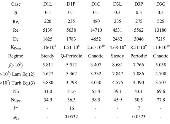
Fig. 1 shows a schematic representation of a closed torus; the torus radius, i.e. the radius of curvature, will be indicated with c, while the cross-section radius with a. The inner side will be indicated with I and the outer side with O; the cross-section azimuthal angle will be measured in a

(10)

clockwise direction looking from upstream, with(I)=-/2,(O)=/2.

A very important engineering application of curved pipes are helical coils, which are used as heat exchangers as well as steam generators in power plant because they are compact and easily accommodate thermal expansion. Several theoretical fundamental studies appeared in the last decades on this geometry (see for example Germano12_{, Chen and Yan}13_{, Jinsuo and Benzhao}14_{); these works} revealed that coil torsion, which characterizes a helical pipe with respect to a toroidal one, has only a higher order effect on flow features, and moderate torsion do not significantly affect global quantities.

1.2. Friction

Pressure drop in slightly curved pipes was first investigated analytically in the creeping region (Larrain and Bonilla10_{), and through the Dean solution (e.g. Van Dyke}8_{, McConalogue and Srivastata}9₎ in the laminar range. The extended Stokes series (ESS) method, developed by Van Dyke8_{on the basis} of the Dean solution, first suggested the friction factor ratio between curved and straight pipes to behave asDe1/4, while boundary layer techniques (Mori and Nakayama15_{) and numerical techniques} (Collins and Dennis16_{) suggested a dependence upon De}1/2 _{for high Dean numbers in the laminar} range. The discrepancy was addressed by Jayanti and Hewitt17 _{and was explained by the relevant} number of terms in the ESS method needed to achieve accurate convergence.

Experimental investigations in a wide range of curvatures and Reynolds numbers were presented by Ito18_{, who derived accurate correlations for the Darcy-Weisbach friction factor f (four times the} Fanning coefficient) in the laminar and turbulent ranges:

5.73 10

64 21.5 De

Re (1.56 log De)

f

 





(Laminar flow) (2) 0.25

0.304 Re

0.029 f

_

_



_



(Turbulent flow) (3)

valid for 5104____{0.2. Eq. (2) shows that for laminar flow the friction ratio can not be accurately} expressed by simple power law behaviour, like in Van Dyke8_{and Collins and Dennis}16_.

Eqs. (2) and (3) have recently been confirmed by the extensive experimental work of Cioncolini and Santini19_{in a wide range of curvatures (2.7}₁₀3____{0.143) and Reynolds numbers (Re=10}3_-7₁₀4_). The authors found a good agreement with Ito’s correlations both in the laminar and in the fully

(11)

turbulent range.

1.3. Transition to turbulence

As regards transition to turbulence, Cioncolini and Santini19_{, for relatively high values of the} curvature (0.04160.143), observed a smooth transition from laminar to turbulent flow; the friction coefficient decreased monotonically with Re and transition to turbulence was indicated only by a change in slope of the f-Re curve. Therefore for high curvatures it is not possible to derive a strict transition criterion based on the friction factor behaviour. Nevertheless, an indicative value of the transitional Reynolds number can be provided by the intersection of fully laminar and fully turbulent asymptotic laws. On the basis of their experimental data, the authors proposed the following correlation for the critical Reynolds number:

0.47

Re

cr



30000





(4)

in the range 0.04160.143. For lower curvatures (<0.0416), the authors observed that in the proximity of transition the f-Re curves exhibited a local minimum followed by an inflection point and by a local maximum; also in this range ofthey proposed transition correlations, more complex than Eq. (4) and based on identifying transition with the local minimum of f, i.e. with the first departure from the laminar behaviour. Similarly, Ito18_{gives an upper bound for the applicability of the laminar} flow friction correlation (2), which can be identified with a transition criterion:



0.6



Re

cr



2000 1 13.2





(5)

in the range 5104____0.2.

Srinivasan et al.20_{studied the transition to turbulence on the basis of friction factor measurements,} and proposed a correlation for the critical Reynolds number in curved pipes:





Re

cr



2100 1 12





(6)

Eqs. (4) through (6) show that the effect of curvature is to increase Recr with respect to straight

pipes. For typical values of the curvature, Eqs. (4) through (6) yield similar values of Recr; for

example, they predict Recr =10 165, 8631 and 10 069, respectively, for=0.1, and Recr = 17 036, 14

(12)

validity of Eqs.(4) and (5); note also that only Eqs. (5) and (6) exhibit a correct asymptotic behaviour for=0 (straight ducts).

A number of two-dimensional studies on transition and stability exist on curved ducts of circular (Dennis and Ng21_{) and square (Wang and Yang}22_{, Daskopoulos and Lenhoff}23_{) cross-section. These} works study by perturbation methods the amplification of disturbances in laminar stationary solutions under the assumption that there is no variation of any quantity along the duct axis. These studies show that four-vortex modes can develop as a second family of solutions at sufficiently high Dean numbers; this four-vortex flow is stable to symmetric disturbances but unstable to asymmetric ones (Yanase et al.24). In this latter work, it is shown that, for circular cross section, the four-cell solution in curved pipes exists only in an open region of the Re-plane and is impossible for Re<252. For example, the critical Reynolds number for the appearance of a second family four-vortex solution is

4

Re

_C



380

for=0.1 and

Re

₄_C



240

for =0.3. These studies have a purely theoretical interest because the perturbation modes found are not the actual three-dimensional modes which develop in a 3-D configuration (e.g. the travelling wave instability modes discussed later on in the present study). As a terminology issue, it is perhaps worth noting that in most works on square cross-section channels (Wang and Yang22_{, Daskopoulos and Lenhoff}23 _{), it is common to call ‘Ekman vortices’ the first} vortices which develop from the imbalance of centrifugal and inertial terms, whose equivalents in circular pipes are the original ‘Dean vortices’ found by Dean7 _{in 1927 and before by Boussinesq}1_{. To} increase the confusion in vocabulary, the same works use ‘Dean vortices’ for the secondary vortices which develop at higher Dean numbers in four-cells or many-cells solutions.

1.4. Heat Transfer

As regards heat transfer, here the classical definition of the Nusselt number for the inner (tube) side will be used:



ˆˆ ˆ2



w b w q a Nu T T



  (7)

(13)

ˆ

w

T

is the wall temperature. In a previous work (Di Piazza and Ciofalo25_{), a systematic computational} study of heat transfer in curved pipes was carried out. The study showed that an excellent reduction of the results data set for the Nusselt number can be obtained by applying the Pethukov momentum -heat transfer analogy (Pethukov26_{) to curved pipes:}

 



2/3



Pr Re / 8 Nu 1.07 12.7 /8 Pr 1 f f     (8)

using Ito’s friction factor correlations, Eqs. (2) and (3), for f. It was shown that this approach is by far superior to any power–law dependence. For Pr1, Eq. (8) approximately reduces to the Reynolds analogy Nu=Re (f/8). Keeping in mind Eqs. (2) and (3), it emerges clearly that in the laminar range, for Pr1, heat transfer is fully governed by the Dean number, i.e. Nu=Nu(De). In the turbulent range, introducing Eq. (3) into the analogy (8) for Pr1 yields

Nu Nu



_s



c

De

, where Nusis the Nusselt number in a straight pipe at the same Reynolds number, and cis a constant. Ref. (Di Piazza and Ciofalo25_{) contains also a thorough review of the literature on heat transfer in curved pipes.}

1.5. Previous CFD studies and experimental works

Numerical simulations of incompressible turbulent flow in helical and curved pipes are presented by Friedrich and co-workers (Hüttl and Friedrich27_{, Friedrich et al.}28_{, Hüttl et al.}29_{). The authors} numerically solve the Navier-Stokes equations written in orthogonal helical coordinates (Germano12₎ and compare toroidal and helical pipe results for Re5600 (Re230) and =0.1. Unfortunately, the authors present statistics of the flow (Reynolds stress distributions in the cross section) for transitional cases which are not turbulent, but rather time-dependent laminar flows. In fact, their test case ‘DT’ is basically coincident in curvature and Re with our case D1P analyzed in the following as a quasi-periodic laminar flow. Thus, the statistics presented in Hüttl and Friedrich27_{and Friedrich et al.}28_can indeed be formally defined and computed but should not be interpreted as proper Reynolds stresses.

Under similar conditions (Re5000-6000,5.510-2_{) a travelling wave instability in helical pipes} was experimentally evidenced by Webster and Humphrey30_{. As recognized by the authors, the} presence of travelling waves makes the length of curved pipe chosen for the experiments a crucial

(14)

parameter, because inlet-outlet conditions will inevitably affect wave length and propagation. For similar reasons, also the CFD simulations documented in Hüttl and Friedrich27 _{and Friedrich et al.}28 would be inadequate to resolve travelling waves, since only a small portion of pipe, 7.5 diameters long, was modelled with periodic boundary conditions and in fact travelling waves are not mentioned in these latter papers.

The possible presence of travelling waves motivated our choice to study via numerical simulation the ideal case of a closed torus, where boundary conditions are not necessary in the axial direction because the domain is circularly closed, and the travelling wave instability can properly develop with a physically consistent wavelength. In the present paper, results for flow in a torus are presented for two values of curvature, i.e. =0.1, 0.3 and three values of the Reynolds number, in the laminar (Re<5200), transitional (Re5200-6000) and chaotic range (Re>6000).

2. MODELS AND METHODS

2.1. CFD Numerical methods

The geometry simulated was a torus (Fig. 1) with no slip conditions at the wall. A constant source term psin the axial momentum equation was adopted as the driving force which balances pressure

drop. This is equivalent to imposing the equilibrium mean shear stress

 

ˆ

₀

_{( / 2)}

a

p

_s and the

corresponding friction velocity

u

ˆ





 

ˆ

0

/

. A friction Reynolds number

Re





u a

ˆ



/



can be defined on the basis of this latter. As thermal boundary condition a constant wall temperature

ˆ

w

T

was imposed. In order to maintain a finite temperature difference between fluid and walls, a local energy source term was applied to compensate, at each time step, the integrated wall heat flux. Due to the definition of the Nusselt number, Eq. (7), based on the bulk temperature

T

ˆ

b, this local source term is

proportional to the local specific mass flow rate in the main flow direction. With this treatment, the fluid energy content, and thus the bulk temperature remain constant during a simulation, and statistically fully developed conditions are obtained. The Prandtl number was fixed to 1 in all cases.

(15)

time-marching algorithm, and a multi-grid approach. The central interpolation scheme was used for the advection terms.

2.2. Computational mesh

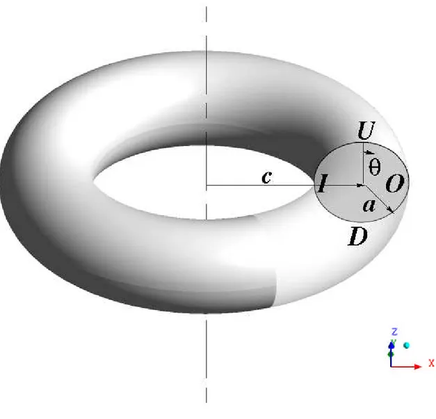
The mesh is multi-block structured, and it is identified by the parameters NRADand Nas shown in

Fig.2. In the present work the values used are NRAD=46, N=24 and a geometric refinement is used at

the wall with a maximum/minimum cell ratio of 5 in the radial direction. With these choices, the cross section is resolved by 11136 cells, and the first point of the grid close to the wall is well within the viscous sublayer (y+__{2.5) at the highest Reynolds number (Re14 000) simulated. In the axial} direction the domain is discretized by NAX=1024 cells for=0.1 and NAX=300 cells for=0.3; this leads

to an overall number of cells of 11.4106_for__{=0.1 and 3.34}₁₀6_for__=0.3. The Kolmogorov length scale

_{( / )}

3 1/ 4

K

 

 

can be computed for the present configuration

as

_{/ Re Re}



1/ 4



K

a



 



; for a resolution of K, the minimum number of cells in half radius can be

computed as MIN

( / 2)/

Re Re / 2

1/ 4

RAD K

N



a

 

_



and the minimu number of cells in the axial direction as MIN

Re Re /

1/ 4

AX

N





_





. In the most critical case (Re14 000), these latter formulae yield MIN

120

RAD

N



and MIN

7540

AX

N



(=0.1) or 2513 (=0.3). Therefore, the present mesh provides a resolution of 2.6K in the radial direction and 78 Kin the axial direction. Taking account of

near-wall grid refinement, these values are of the same order as those usually adopted in Direct Numerical Simulation of turbulence (Kim et al.31_{). The time step was set at most equal to 0.8(/u}

2) for all cases;

this time discretization is sufficient to capture both turbulent variations (Choi and Moin32_{) and the} dynamic features of laminar time-dependent flows. It should be stressed that in the present work emphasis is placed on these latter rather than on fully turbulent flows. For the present axial grid, the above criterion is basically equivalent to that of a Courant number less than 1 in all cases.

Zero velocity and uniform temperature initial conditions were set for all the numerical simulations. Instabilities, if present, were spontaneously triggered by small numerical fluctuations due to truncation and round-off errors.

(16)

2.3. Scales and frames of reference

Although the friction velocity

u

ˆ

_is the a-priori known quantity (due to the source term imposed in the momentum equation), the average velocity

u

ˆ

_av was chosen as the velocity scale. This is because for any curvature the velocity of the Dean vortex scales with

u

ˆ

_av, as shown by Eq. (1).

The corresponding frequency scale of the Dean circulation can be computed as:

0 2

ˆ

De

ˆ

2

av

u

f

a









(9)

which reflects the number of turns of the Dean vortex per unit time. This frequency scale can be viewed also as an amplification, by a factor proportional to the Dean number, of the molecular momentum diffusion frequency

_

_{/ a}2_{. The time scale follows as}

0

ˆ

0

ˆ 1/

t



f

. The scale for angular velocity is naturally



ˆ

0



2 f



ˆ

0.

The non-dimensional temperature T was computed as

(

T T

ˆ ˆ ˆ ˆ



w

) /(

T

b



T

w

)

; the turbulence energy was scaled by

_ˆ

2

av

u

, while pressure and wall shear stress were scaled by

_ˆ

2

av

u



. All coordinates were scaled by the cross section radius a; the non-dimensional radial coordinate measured from the torus axis is

r

p



r a

ˆ

p

/

, while the non-dimensional local radial coordinate, measured from the centre of the cross section, is r r aˆ/ . Assuming a cylindrical general frame of reference (rp,, z) for the torus,

and a local 2-D polar frame of reference (r, ) for the cross section, one has

r

p



r

sin( ) 1/







and

cos( )

z r



. The local Nusselt number Nu and non-dimensional wall shear stress



ware computed

as:

Nu( ) 2

w

dT

dr

 

(10)

2 ( )

Re

w w

du

dr

   

(11)

(17)

2.4. Proper Orthogonal Decomposition

The Proper Orthogonal Decomposition (POD) technique was used to post-process the raw simulation results in the generic cross section. This technique was introduced in the study of turbulent flows by Lumley33_{and a complete description is given by Berkooz, Holmes and Lumley}34_{; it is also} used with other names (Principal Component Analysis, Karhunen-Loève Transform) in several disparate research fields like meteorology and psychology. It is based on a two-point correlation and is able to capture the highest possible variance of the system with the least possible number of orthogonal eigenfunctions.

For a 2-D time-dependent problem, eigenvalues iand eigenfunctions i(x,y) are computed from

the time-covariance matrix built with the raw data, which leads to the following decomposition:

1

( , )

N i

( )

i

( , )

i

u

u x y

a t

x y













(12)

whereu x y( , )is the time-averaged field of a generic quantity u while the generic term ai(t)i(x,y) is the product of the i-th time-dependent coefficient by the i-th spatial eigenfunction. This

decomposition does not postulate a particular shape for i(x,y), but finds the ‘natural’ spatial

eigenfunctions of the system in a specific flow condition; the modes which posses the highest variance (energy in the case of a velocity field) can be captured and separated from one another. In this way, the time-dependent field can be filtered using only the first, highest-variance, N eigenfunctions. The quantity

 

i



i

/





irepresents the fraction of variance described by the i-th eigenfunction.

An in-house computer program was developed to perform numerically the Proper Orthogonal Decomposition on arbitrary data sets. The software is able to treat 2-D or 3-D fields and extracts all the eigenvalues and eigenfunctions of the two-point correlation matrix. The time-dependent coefficients ai(t) are computed by projecting the original data set into the new eigenfunctions basis.

2.5. Range of parameters explored

In the present study, a systematic investigation in the range Re=220-525 was carried out for the curvatures =0.1, 0.3. The range was investigated by letting Revary in steps, and the following conclusions were derived on the different regimes:

(18)

 The transition is governed by the flow Reynolds number Re;

 Laminar stationary solutions were encountered for Re<5200 for both curvatures;  Periodic or quasi-periodic flows with single spectral peaks, associated with travelling

waves, were found in the range 5200<Re<6000;

 For Re>6000 chaotic phenomena progressively started while the Reynolds number increased; a continuous fluctuation spectrum, characterizing a fully turbulent flow, was obtained for Re>10 000.

Table 1 summarizes the six selected test cases presented in this paper. They cover two values of the curvature, i.e. =0.1 and 0.3, denoted by D1 and D3, and three different regimes, i.e. stationary laminar, transitional (periodic or quasi-periodic) and chaotic (turbulent), denoted by L, P and C, respectively. Both Reynolds numbers Re and Reare provided in Table 1 for the sake of completeness; the friction factor can be computed simply by f=32(Re/Re)2, and its values predicted by Ito’s resistance correlations (2) and (3) are also reported. For future comparison with other works, the Dean number De, as defined in section I, and the Dean number KDean originally introduced by Dean7_{, are also reported. The latter form of the Dean number is based on the pressure gradient, and} can be related to the other non-dimensional parameters as

K

_Dean



(

p a

s2 7

) /(8



2 4

c

) (1/ 2)Re



4



(Berger et al.11_).

3. STATIONARY LAMINAR CASES (D1L-D3L)

The main reason to discuss stationary laminar results is to establish a basis of comparison for the subsequent unsteady solutions presented in section IV. Of course, since these solutions are strictly 2-D, a fully 3-D simulation would not be necessary, but this can be stated only by hindsight.

The results presented here are for Re=5139, =0.1 (case D1L) and Re=4531, =0.3 (case D3L). The corresponding Darcy-Weisbach friction factor and mean Nusselt number are summarized in Table 1; the higher values found in D3L with respect to D1L are justified by the higher Dean number, and thus the more intense secondary circulation at higher curvatures.

(19)

self similar for different Re and given(McConalogue and Srivastata9_{), as confirmed by the fact that} the f/fs ratio, Eq. (2), varies with

De Re 



and thus varies with Re for any given . This is

equivalent to saying that the pressure drop in curved pipes is not proportional to the flow rate even in steady laminar flow.

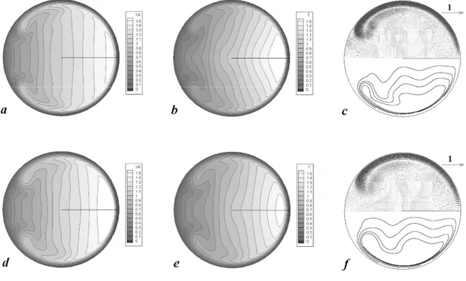
Fig. 3 shows the non-dimensional solutions in the cross-section for D3L (top row) and D1L (bottom row). The graphs in the first column (a, d) report contours of the axial velocity us, those in the

second column (b, e) contours of the temperature T. The graphs in the third column report vector plots of the secondary motion in their top half, with the reference unitary vector drawn, and corresponding streamlines in the bottom half. It can be observed that the Dean vortex is smaller but stronger for D3L with respect to D1L, with the iso-lines more stretched in the near-wall region by the secondary flow; for each curvature, temperature and velocity fields appear similar in the Dean vortex region and in the secondary wall boundary layer.

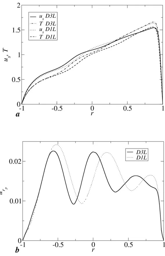
Fig. 4(a) shows profiles of axial velocity usand temperature T along the equatorial midplane I-0

for D3L and D1L. Once made dimensionless, all profiles collapse on a similar roughly linear behaviour characterized by a slope 3/4. It should be observed that in a rigid-body rotation the dimensionless slope would be O(), i.e. much smaller. Increasing the curvature results only in a moderate increase of the peak usand T near the outer wall and in a moderate decrease of usand T near

the inner wall. The behaviour of usin the core region can be related to that of the radial velocity urp

(referred to the torus radius) by an inviscid balance between inertial forces and pressure drop, which can be approximately written as:

2

ˆ ˆ

/

(2 / ) ( / )

s p rp av

u

r

u

u u

_

  



(13)

This balance expresses the physical elementary mechanism that shifts the axial velocity maximum towards the outer wall.

Fig. 4(b) shows the radial velocity urpalong the I-0 line. In the core region this quantity oscillates

around 0.015, yielding

  

u

_s

/

r

_p

1

which is of the correct order; the relative maxima and minima of urpin Fig. 4(b) correspond to the minima and maxima in the slope of the velocity profiles in Fig. 4(a),

(20)

4. PERIODIC AND QUASI-PERIODIC CASES (D1P-D3P)

This section will be devoted to a thorough analysis of cases D1P, D3P of Table 1. In a closed torus, the Dean cells form closed symmetric vortex tubes in the laminar-stationary range. As the Reynolds number increases, these vortex tubes become unstable and varicose modes develop; this yields a travelling wave instability moving inside the toroidal waveguide. Being Pr=1 for the present cases, heat and momentum have the same molecular diffusivity. Therefore, the temperature T can be regarded as a tracer to evidence the flow structures.

4.1. Curvature =0.3 (case D3P) a) Flow features

For the higher curvature, a Hopf bifurcation with the onset of periodic flow and simultaneous break-up of the symmetry between the upper and lower halves of the torus occurs for Re>5200. Examples of instantaneous temperature fields in the generic cross section, computed for Re=5562, case D3P, are shown in Fig. 5; (a) and (b) represent instants of time separated by half a period. In the generic cross section, the Dean vortices located in the upper part and in the lower part vary periodically in intensity, coupled in phase opposition: when the upper vortex grows, the lower vortex decreases in intensity, and viceversa. This corresponds to a break-up of instantaneous symmetry and to a periodic single-mode motion. At any instant, the 3-D flow field is spatially periodic along the torus; it moves rigidly in the flow direction along the toroidal channel as a travelling wave whose angular celerity differs from the average convective angular velocity of the fluid. This can be regarded as a travelling varicose instability of each Dean vortex tube, as anticipated above. The temperature field in a plane parallel to the torus midplane, and the vertical velocity field in the midplane are shown in Figs. 6 (a) and (b) respectively; the scales were chosen to evidence the trace of the spatially periodic travelling structure with k*_{=7 waves in the whole torus. The non-dimensional angular celerity (scaled}

by



₀



₂



u

ˆ

_av



_/

a

) is 2=0.0523. The non-dimensional frequency associated with the transit of

(21)

any time-dependent quantity at a fixed point. If the wave celerity coincided with the average axial velocity of the fluid, its non-dimensional frequency would be



₂_fl



 

/ 2



0.0872

; therefore in this case the wave is slower than the fluid in the average, being



₂





_{2 fl} . As a consequence, the wave will lead the fluid only in low speed regions (e.g., near the walls) but will lag behind the fluid over most of the domain.

b) Analysis by Proper Orthogonal Decomposition

Following Eq.(12), the time dependent field can be decomposed via POD into the time-averaged field and a series of spatial eigenfunctions i(x,y) times time-dependent coefficients ai(t). Applying

POD to the two-dimensional axial velocity field in a generic cross section of the torus, the periodic mode emerges clearly. In fact, the first two eigenfunctions resulting from the analysis capture about 96% of the energy, as shown in Table 2, where the first 6 eigenvalues are reported; the residual portion can be interpreted as numerical noise. Two is the minimum number of terms required to describe the periodic change in shape that represents the cross sectional trace of a coherent structure travelling through the domain; the two terms together make up a single mode. This is an important property which seems to have been overlooked in the POD literature.

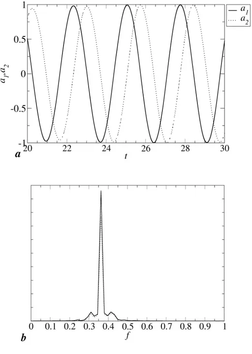
Fig. 7 shows, from (a) to (c), the time-averaged axial velocity field and the first two eigenfunctions 1,2, while the corresponding time-dependent coefficients a1(t), a2(t) are shown for

some periods in Fig. 8(a). The time-averaged cross-section field, Fig. 7(a), is similar to that discussed above for the same and stationary solutions, Fig. 3(a). The eigenfunctions spatially localize fluctuations, which are of the order of 0.06 in dimensionless amplitude, and identify the alternate pulsation of the Dean vortices; no fluctuations exist in the outer region, coherently with what was observed in some experimental work (Webster and Humphrey30_{). Each eigenfunction, and thus the} global fluctuation field, is anti-symmetric with respect to the section midline I-O, i.e.

( , )

i

r z

p i

r

p

z







. The Fourier spectra of a1(t), a2(t) are shown in Fig. 8(b); there is a clear

spectral peak at f10.36, as it was previously predicted by the kinematic analysis of the travelling

(22)

almost perfectly sinusoidal functions sharing the same period and shifted in phase with respect to each other. This corresponds to the fact that the varicose travelling modes in the upper and lower Dean vortex tubes are spatially shifted by half wavelength. As a consequence, the overall flow field possesses the semi-periodicity property with respect to the vertical direction z and time, i.e., for any quantity ,



( , , )

r z t

_p



( , ,

r

_p

 

z t



/ 2)

where the sign + is for

u u T

_s

, ,

_r while the sign – is for

,

z

u u

_and vorticity, and is the dimensionless time period.

A phase-space projection of the system’s trajectory is shown in Fig. 9, where axial velocities at two different points of the domain are plotted one against the other; the graph shows clearly that the system’s attractor appears almost exactly a limit cycle.

4.2. Curvature =0.1 (case D1P) a) Flow features

Also for the lower curvature examined in this paper, i.e. =0.1, a transition from steady to time-dependent flow occurs as Re>5200. However, in this case the instantaneous distributions of any quantity over the generic cross section exhibit symmetry with respect to the torus equatorial midplane, as shown in Fig. 10(a) and (b) which reports temperature at different instants of time for case D1P (Re=5638).

The transition results in a more complex system of travelling waves than in the higher curvature case D3P. The main axial travelling wave is present again, as in D3P. The trace of the three dimensional axial wave in the torus equatorial midplane is shown in Fig. 11(a) by reporting the instantaneous map of temperature. Here, k*_{=16 periodic cells can be visualized in the whole torus.}

This structure travels in the same direction as the mean flow (anti-clockwise in this case) with a non-dimensional angular celerity 2=0.0532, very close to that obtained in D3P (2=0.0523). This

angular celerity is also similar to that found experimentally in Webster and Humphrey30_{, where a} dimensionless value of about 0.05 was measured; the value k*_{=19 obtained in Webster and}

Humphrey30 _{for a lower curvature is also consistent with the present results. The non-dimensional} frequency associated with the transit of one of the periodic is fI=k*2=0.852. This mode ‘I’ is

(23)

associated with the pulsation of the Dean vortices which now, however, occurs in phase between the upper and lower halves of the torus. In this case, if the wave celerity coincided with the average axial velocity of the fluid, its non-dimensional angular celerity would be



₂fl



 

/ 2



0.0503

for

=0.1. Therefore, the wave celerity is close to the mean fluid velocity and the wave will lead the fluid in the inner region while it will lag behind it in the outer region.

A second, weaker, mode can be discovered by looking, for example, at the temperature field on a concentric torus of radius r=0.9, as shown in Fig. 11(b). By using pictures like this latter and building an animation in the Lagrangian frame of reference of the travelling wave ‘I’, a new oblique wave ‘II’ appears within each of the k*_{cells, travelling (with respect to wave ‘I’) in the direction indicated by}

the arrow in the figure. From a visual analysis of such animations, a Lagrangian non-dimensional frequency L

II

f

can be measured. Indicating with

c c

ˆ ˆ

I

,

II the dimensioned celerities of the travelling

waves of mode ‘I’ and ‘II’, and with

L L

ˆ ˆ

_I

,

_II the corresponding dimensional wavelengths, the above

frequency, in dimensional form, can be expressed as:

ˆ

L

₍

ˆ ˆ

_{) /}

ˆ

II I II II

f

 

c

L

; the corresponding dimensionless expression is:

L I II II II

c

f

L







(14) where 2 *

2

* II II II

L

k









(15) and * II

k

is the number of oblique waves in the whole torus. Once L

, ,

II I II

f c L

are known, the dimensionless wave celerity cIIof the oblique wave can be derived. In

the present case, *

2

1.278,

(2 /

) 1.057,

36,

1.745

L

II I II II

f



c



f

_

 



k



L



, and thus cII=0.352.

The frequency of the second (oblique) mode in the laboratory frame of reference is now:

0.638

II II II

c

f

L







(16)

Thus the frequency of mode ‘II’ is lower than that of mode ‘I’ and, to the degree of accuracy allowed by numerical simulations, the two frequencies appear incommensurate, which corresponds to a quasi

(24)

periodic flow.

b) Analysis by Proper Orthogonal Decomposition

The two modes can be better characterized by applying POD analysis to the cross-section, similarly to what was done for case D3P. Table 2 reports the first 6 eigenvalues of the axial velocity. Eigenvalues 1 to 4 collect about 82% of the energy. Fig. 12 from (b) to (e) shows the corresponding spatial eigenfunctions from 1 to 4 for the axial velocity, while Fig. 12(a) is its time-averaged distribution. Eigenfunctions 1 (Fig. 12(b)) and 2 (Fig. 12(c)) are mostly associated with mode ‘I’, i.e. with the axial travelling wave related to Dean vortex pulsation. In this case the maxima are located in the vicinity of the Dean vortices; mode ‘I’ carries about 67% of velocity variance. Eigenfunctions 3 (Fig. 12(d)) and 4 (Fig. 12(e)) are mostly associated with mode ‘II’, and represent a trail of near -wall vortices which are produced in the Dean vortex areas, and travel from I to O, i-e- upstream with respect to the secondary flow boundary layers, at the edge of these latter, following the wall curvature. This latter mode carries about 15% of the velocity variance, and thus it is much less energetic than mode ‘I’. Fig. 13 represents the POD decomposition of the vorticity normal to the cross-section: Fig. 13(a) is the average field while Figs. 13(b) to (e) are the eigenfunctions from 1 to 4. Vorticity eigenfunctions are anti-symmetric with respect to the I-O horizontal line, and exhibits more clearly than velocity the separation of modes; mode ‘II’ exhibits about three times more vorticity variance (enstrophy) than mode ‘I’, in opposition to what happens for the velocity variance (energy). This is coherent with the smaller spatial scale associated with mode ‘II’.

Figs. 14(a) and (b) show time-dependent vorticity coefficients a1,a2(a) and a3,a4(b), over an

arbitrary time interval. The coefficients a1-a2, mainly associated with mode ‘I’, and a3-a4, mainly

associated with mode ‘II’, are characterized by a different periodicity. In Fig. 14(c), the spectrum of the vorticity coefficients is shown. Frequencies associated to mode ‘I’ and ‘II’ clearly emerge respectively as fI0.87, fII0.64, as derived above from a wave kinematic analysis based on flow

visualization.

Fig. 15 shows temperature at a point against velocity at another point (arbitrary units); the graph represents a projection of the system’s trajectory onto a 2-D subspace. The figure illustrates as the

(25)

orbits approaching a limit cycle existing in the periodic case D3P, characterized by a single frequency, are replaced by orbits which do not exactly repeat themselves at each turn and approach a torus attractor characteristic of a quasi-periodic behaviour with two incommensurate frequencies. This effect is entirely due to the second frequency fIIappearing in the present case D1P.

c) Comparison with previous numerical results and experimental data

Fig. 16 shows a comparison between present results and computations presented by Friedrich and co-workers (Hüttl and Friedrich27 _{and Friedrich et al.}28_{) for} __{=0.1 and Re5632 (Re}

230). The comparison is made on the time-averaged fields. As discussed in Section I.A, the authors simulated a tract of a toroidal pipe, 7.5 diameters in length, whereas in the present simulations the computational domain included the whole torus.

Fig. 16(a) shows the axial velocity versus the non-dimensional radial coordinate r along the equatorial line I-0 of a cross section, from the inner wall (r=-1) to the outer wall (r=1) and along the vertical midline from the wall (r=-1) to the centre of the section (r=0); in the latter case the problem is symmetric in the average with respect to the torus midplane so that only one half of the graph needs to be reported. Symbols denote the experimental results presented by Webster and Humprey30 _for Re=5480 and=5.510-2_{. The agreement is very good with the numerical simulations and fair with the} experimental data (taken with a different curvature). It should be noticed that the radial gradient of the axial velocity along the I-0 line in Fig. 16(a), once made dimensionless, is 3/4, as in the stationary laminar cases. Fig. 16(b) shows a comparison for the time-averaged radial profile of the azimuthal velocity along the U-D line, see Fig. 1. It shows a characteristic peak associated with the secondary stream boundary layer; the agreement with numerical results in Hüttl and Friedrich27_{and Friedrich et} al.28 is fully satisfactory also for this quantity. Fig. 17 shows profiles of dimensionless fluctuation kinetic energy K along the I-O and D-U midlines of a cross section. Present results are compared with the numerical predictions in Hüttl and Friedrich27 _{and Friedrich et al.}28_{. There is a general good} agreement of the profiles, and the main differences are located in the outer region for the I-O line and in the boundary layer peaks for the D-U line.

(26)

field (b), (e) and secondary flow field (c), (f) in a cross section for cases D3P (first row) and D1P (second row). The graphs (c) and (f) report velocity vectors in their upper half and streamlines of the secondary flow in their lower half. Time-averaged results are very similar to those obtained for the stationary cases D3L and D1L, and similar considerations yield. Therefore the travelling waves only ‘disturb’ the stationary solution, and cases D3P and D1P, far to be turbulent, can be classified as time-dependent laminar flows.

5. CHAOTIC FLOW

In this section, results for the fully turbulent cases D1C and D3C (Re13000-14000) will be presented. In contrast with straight pipe turbulence, where fluctuations are azimuthally uniform, in curved pipes they are localized mainly in specific regions, where particular flow featurwes, such as Dean vortices, occur.

For these chaotic cases, first- and higher-order statistics can be computed from time-dependent results. The spectrum of the axial velocity at a monitoring point for case D3C is shown in Fig. 19; it appears almost continuous and a wide range of frequencies are present, with a small but recognizable inertial sub-range with the characteristic slope -5/3. A similar behaviour holds for case D1C. Also Proper Orthogonal Decomposition, once applied to these chaotic cases, shows a continuous eigenvalues spectrum; the first 600 eigenmodes collect 99% of the energy. Therefore, cases D3C and D1C can be characterized as fully turbulent.

From a phenomenological point of view, middle-size vortices are continuously produced throughout the cross section, as shown by instantaneous vector plots for cases D3C and D1C in Fig. 20. However, time-averaged flow fields, as reported in Fig. 21, show that almost all structures average out leaving the Dean vortices in the usual locations near the inner wall, and, only in the high curvature case, a weaker counter-rotating couple of vortices near the outer wall. These small vortices are reminiscent of the structures predicted by Dennis and Ng21_{and by Yanase et al.}24_{in their four-vortex} family of solutions for laminar flow in curved circular pipes. However, in the present simulations such other-side vortices only emerge as time-averages of turbulent flow, and were not obtained in

(27)

steady-unstable to disturbances which are asymmetric with respect to the midplane. Although both cases exhibit instantaneous lack of symmetry, in the average flow symmetry is recovered. The same conclusions can be drawn by looking at time-averaged maps of axial velocity and temperature, Fig. 22. As for the transitional cases, the detachment angle of the Dean vortex is lower for the lower curvature, i.e. the secondary vortex is larger for=0.1.

The dimensionless time-averaged axial velocity and temperature along the I-0 line is shown in Fig. 23(a). Both temperature and velocity stratification is O(1) in dimensionless form, as in the stationary flow results presented in Fig. 4(a). Fig. 23(b) reports the time-averaged radial velocity urp

along the same I-O line. In the proximity of the outer wall urp is always positive (i.e., directed in the

I-0 direction) for the low curvature case D1C, whereas it becomes negative ine the region 0.5<r<0.8 for the high curvature case D3C, in correspondence with the existence of the above mentioned counter-rotating secondary vortices in the time-mean flow. In the core region, profiles of the axial and radial velocity components are approximately related by the same inviscid balance discussed for the case of stationary flow, see Eq. (13) and Fig. 4.

Fig. 24 shows the distribution of dimensionless kinetic energy K, fluctuating pressure pRMS and

fluctuating temperature TRMS for cases D3C and D1C. The highest values of turbulent kinetic energy

are located in the outer region, in the upper and lower wall streams and in the Dean vortex region. Therefore, the secondary flow, although much less intense than the main flow in the average, plays an important role in causing the distribution of turbulence intensity over the cross section. As it was expected, fluctuation levels are higher for the higher curvature; thus, despite the stabilizing effect of curvature as regards transition, reflected in Eqs. (4) through (6), curvature enhances the levels of turbulence once it is established, as confirmed by its effects on friction and heat transfer.

A projection of the system trajectory on a 2-D subspace for D3C is shown in Fig.25; the trajectory, as it was expected, appears chaotic, confirming the turbulent nature of the flow at these Reynolds numbers.

6. OVERALL ANALOGIES

(28)

represented in Fig. 26. In all cases, the higher curvature=0.3 has a higher dimensionless wall shear stress with respect to=0.1. In the turbulent cases (D3C, D1C), the azimuthal profile is flatter than in laminar and transitional ones (D3P, D3L, D1P, D1L). For each case, the w profile grows

monotonically from =-45° to =90°; the maximum at =90° corresponds to the outer wall region. This behaviour reflects the I-0 stratification of the axial velocity.

Corresponding profiles of the local Nusselt number are shown in Fig.27. The higher curvature geometry exhibits higher values of Nu for all flow regimes. The local minimum of the curves around

=60° marks the detachment point of the Dean vortex. Remarkably the detachment angle is about -60°, very close to that predicted by the boundary layer integral asymptotic model of Barua34_{for high} Reynolds numbers. The local Nusselt number grows from I to O, in analogy with momentum transfer, and is associated with the temperature stratification in the I-0 direction. As shown in a recent work (Di Piazza and Ciofalo25_{), a modified Reynolds analogy is applicable to curved ducts for heat transfer.} This is valid in the average, but it is still approximately valid also locally, as shown in Fig. 28, where the ratio

Nu

( ) /( ( )Re Pr)

  

w is reported against the azimuthalangle for all cases simulated here.

For the lower curvature, the ratio varies from 0.8 to 1.2, while for the higher curvature (=0.3), the analogy is less applicable, and the ratio ranges from 0.7 to 1.4. The analogy between momentum and heat transfer explains why the non-dimensional profiles of velocity and temperature shown throughout the paper are similar and exhibit the same stratification.

Focussing the attention on the I-0 midline, it is interesting to investigate the local momentum equilibrium. Along this line, in the core region far from the boundary layer, both convective and viscous terms are unimportant, so that an inviscid balance between pressure gradient and centrifugal forces approximately yields:

2 s p

u

p

r

 



(17)

This is shown in Fig. 29(a), where the ratio

 

u r

2s

/

p

/



 

p r

/



is plotted along the I-0 line. The ratio is O(1) from r=-0.75 to r=0.75, i.e. in the core region, for all cases examined (laminar, transitional and turbulent flow). As a consequence of the momentum-heat transfer analogy discussed

(29)

above, for Pr1 the pressure gradient in the core region is tied both to the velocity and to the thermal stratification, i.e.

_/

2

_/

2

_/

s p p

p r u r

T

r

  



. Considering that both axial velocity and temperature exhibit a linear stratification with a slope b3/4 regardless of the Reynolds number, see Figs. 23(a) and 4(a), by integrating the inviscid balance in Eq. (17) it can be shown that, in the core region and in dimensionless form, for<<1, the pressure profile can be approximated as

2

3 2

3 p

b

_r

_br

_r







(18)

This is valid both for laminar stationary cases and for the time-averaged field in the transient and chaotic cases as shown in Fig. 29(b), where all the time-averaged profiles p/are compared with the above-mentioned analytical expression. The agreement is better around r=0 where the inviscid balance is more closely valid.

7. CONCLUSIONS

Time-dependent numerical simulations were conducted for flow and heat transfer in toroidal pipes. A constant property fluid with Pr=1 was assumed. Two curvatures (=0.1 and 0.3) were examined. A streamwise driving pressure gradient was imposed and its magnitude was made to vary in steps so that the friction Reynolds number

Re

_



u a

_

/



spanned the range 220 to 525, yielding flow Reynolds numbers between 4531 and 14710, and Dean numbers

De Re 



between 1625 and 7219.

A finite volume method was used; the computational domain included the whole torus and was discretized by 3.4106 _{nodes for the higher curvature (}__{=0.3) and 11.3}₁₀6 _{nodes for the lower one} (=0.1).

Transition between different flow regimes was found to be controlled by the Reynolds number. For Re<5200, stationary flow was predicted, exhibiting the general properties well documented in the literature for steady flow in curved circular pipes. For Re>6000, the flow became chaotic and exhibited a broad frequency spectrum, although it became fully turbulent, with an inertial sub -range and overall properties (f, Nu) typical of turbulent flows in curved pipes, only for Re>10 000.

(30)

In the narrow intermediate range 5200Re6000, a more complex behaviour was predicted. In this range, the nature of the flow was identified and quantitatively characterized by the simultaneous use of different techniques including static and dynamic flow and scalar (T) visualization on different sections of the torus; Proper Orthogonal Decomposition; spectral analysis; and projections of the system’s trajectories on 2-D variable sub-sets.

For the higher curvature (=0.3) the flow exhibited a periodic behaviour, with a single sharp peak in POD spectra and a limit-cycle attractor in phase space. Periodicity was associated with a varicose instability of the twin toroidal Dean vortices, propagating streamwise along the flow direction as a couple of travelling waves in opposition of phase with respect to each other. This behaviour is indicative of a Hopf bifurcation occurring at Re5200 and yielding distributions of flow and temperature which were instantaneously asymmetric with respect to the equatorial plane in each cross section. The number of wavelengths associated with this varicose instability was 7 (in 2) in this range of the Reynolds number.

For the lower curvature (=0.1), the flow followed a nearly quasi-periodic behaviour, characterized by the existence of two incommensurate peaks in frequency spectra and by a torus attractor in the appropriate phase space. The higher frequency mode (mode ‘I’) was associated with a travelling wave similar to that observed in the previous, high curvature, case, but symmetric with respect to the equatorial midplane of the torus and thus yielding instantaneous cross-section distributions which preserved up-down symmetry. The number of wavelengths associated with this mode was 16 in 2. The lower-frequency mode (mode ‘II’) was associated with oblique waves propagating mainly in the top and bottom near-wall regions adjacent to the Dean vortices; in each cross section, it appeared as a couple of trails of weak vortices, detaching themselves from each Dean vortex and travelling along the walls from the inner to the outer pole, i.e. against the secondary near-wall streams. Mode ‘II’ contained less velocity variance (energy), but more vorticity variance (enstrophy), than mode ‘I’.

For both curvatures, the angular celerity of the main travelling wave associated with the instability of the toroidal Dean vortices scaled well with the Dean number, in agreement with the experimental findings of Webster and Humprey30_.

(31)

The radial stratification of axial velocity and temperature in the core flow was approximately described by a linear behaviour with the same dimensionless slope of O(1) in all cases. The relation between axial velocity, radial velocity and pressure gradient in the core flow was found to be mainly governed by inviscid balances for all flow regimes.

As a conclusive remark, it must be pointed out that the results presented in this work and their physical interpretation have mainly an exploratory value, are limited to a small number of test cases and thus do not have the ambition of being exhaustive. Further systematic investigations may be needed to achieve a full classification of flow regimes in toroidal pipes.

Similar remarks hold as regards the extension of the present results to the case of helical pipes (coils with non-zero pitch). While experimental results like those by Webster and Humprey30_suggest that travelling waves occur also for finite pitches, it is clear that the details of these intermediate flow regimes and of their transitions will depend on the specific pich considered and may exhibit different features, which can be clarified only by further direct numerical simulations.

(32)

REFERENCES

1_{M.J. Boussinesq, “Mémoire sur l’influence des frottements dans les mouvements régulier des fluids”,} Journal de Mathématiques Pures et Appliquées 2me Série 13, 377 (1868).

2_{J. Thomson, “On the origin of windings of rivers in alluvial plains, with remarks on the flow of water} round bends in pipes”, Proc. R. Soc. London Ser. A 25, 5 (1876).

3_{G.S. Williams, C.W. Hubbell and G.H. Fenkell, “On the effect of curvature upon the flow of water in} pipes”, Trans. ASCE 47, 1 (1902).

4_{J.H. Grindley and A.H. Gibson, “On the frictional resistance to the flow of air through a pipe”, Proc.} R. Soc. London Ser. A 80, 114 (1908).

5_{J. Eustice, “Experiment of streamline motion in curved pipes”, Proc. R. Soc. London Ser. 85, 119} (1911).

6_{A. Einstein, “Die Ursache der Mäanderbildung der Flußläufe und des sogenannten Baerschen} Gesetzes”, Die Naturwissenschaften 11, 223 (1926).

7_{W.R. Dean, “Note on the motion of the fluid in a curved pipe”, Phil. Mag. 4, 208 (1927).}

8_{M. Van Dyke, “Extended Stokes series: laminar flow through a loosely curved pipe”, J. Fluid Mech.}

86, 129 (1978).

9_{D.J. McConalogue and R.S. Srivastata, “Motion of fluid in a curved tube”, Proc. Real Soc. London} Ser. A 307, 37 (1968).

10_{J. Larrain and C.F. Bonilla, “Theoretical analysis of pressure drop in the laminar flow of fluid in a} coiled pipe”, Trans. Soc. Rheol. 14, 135 (1970).

11_{S.A. Berger, L. Talbot and L.S. Yao, “Flow in curved pipes”, Ann Rev Fluid Mech 15, 461 (1983).} 12_{M. Germano, “On the effect of torsion in a helical pipe flow”, J. Fluid Mech. 125, 1 (1982).}

13_{W.H. Chen and R. Jan, “The characteristics of laminar flow in helical circular pipe”, J. Fluid Mech.}

Modelling flow and heat transfer in helically coiled pipes - Part 2: Direct numerical simulations for laminar, transitional and weacly turbulent flow in the case of zero pitch

CIRTEN

C

I

R

T

N