Contents lists available atScienceDirect
Operations Research Perspectives
journal homepage:www.elsevier.com/locate/orp
Optimal paths in multi-stage stochastic decision networks
Mina Roohnavazfar
a,c, Daniele Manerba
a,b, Juan Carlos De Martin
a, Roberto Tadei
⁎,a aDepartment of Control and Computer Engineering, Politecnico di Torino, Corso Duca degli Abruzzi, 24, Torino 10129, ItalybICT for City Logistics and Enterprises Lab, Politecnico di Torino, Turin, Italy cDepartment of Industrial Engineering, Kharazmi University, Tehran, Iran
A R T I C L E I N F O Keywords:
Optimal paths
Stochastic decision process Multi-stage
Asymptotic approximation Nested Multinomial Logit
A B S T R A C T
This paper deals with the search of optimal paths in a multi-stage stochastic decision network as a first application of the deterministic approximation approach proposed by Tadei et al. [48]. In the network, the involved utilities are stage-dependent and contain random oscillations with an unknown probability distribution. The problem is modeled as a sequential choice of nodes in a graph layered into stages, in order to find the optimal path value in a recursive fashion. It is also shown that an optimal path solution can be derived by using a Nested Multinomial Logit model, which represents the choice probability at the different stages. The accuracy and efficiency of the proposed method are experimentally proved on a large set of randomly generated instances. Moreover, insights on the calibration of a critical parameter of the deterministic approximation are also provided.
1. Introduction
Finding optimal paths is one of the most fundamental problems on graphs with broad applications in various fields like computer science, robotics, operations research, and transportation planning. The pro-blem can be seen as a multi-stage decision process in which decisions are made step by step to eventually achieve an optimal sequence of choices, i.e., an optimal path throughout the stages. Depending on the application, the objective may be expressed in terms of maximization of utilities or minimization of costs, which in turn may lead to search for the most-profitable or the less-costly path on a graph, respectively. Note that the most-profitable path can be seen as the longest path when the arc utilities are substituted with arc costs, while the less-costly path actually corresponds to the shortest path. In this paper, we mainly provide a detailed approach for the former case, while for the latter we just briefly discuss those assumptions that allow just a symmetric ap-plication of the same conceptual framework.
Most of the operations management areas such as logistics, routing, scheduling, project management, and finance face concrete settings which lead to the problem of finding an optimal sequence (path) of decisions over alternatives in a multi-stage framework. In these pro-blems, the utility of a choice at each stage is affected by the utilities associated to the selected choices in the subsequent stages. In this sense, decision making over stages leads to finally look for an optimal path made by the choices selected stage by stage in a sequential fashion. Actually, the idea of using a sequential decision making model to
describe a path has been around for quite some time (see, e.g., [1,6,16]). We want to highlight since now that, depending on the dif-ferent application at hand, the concept of stage may represent difdif-ferent discretization of the decision problem, and not necessarily a dis-cretization of the time horizon. A clear example can be found in some project management problems presented inSection 2.5, in relation to the well-known Critical Path Method.
When all parameters of the application are deterministically known a priori, finding optimal paths is in general an easy problem to solve. However, in most real-life settings, parameters are highly affected by uncertainty and, moreover, there might be circumstances in which parameters are being changed dynamically over the decision horizon. It is easy to understand that, in those cases, ignoring the parameter variability may lead to inferior or, even worse, simply wrong decisions. It is also well-known that explicitly addressing uncertainty in an opti-mization problem generally increases the complexity of the decision making process and poses significant computational challenges. Therefore, it always makes sense to see whether it is possible to in-corporate stochasticity in an approximated way, converting the sto-chastic multi-stage model into a deterministic one and, if so, how ac-curate this approximation is.
In this paper, we define the optimal path problem as a multi-stage decision process where the choice utilities are varying over stages and are also assumed to be stochastic variables with an unknown prob-ability distribution. This work provides the first application of the multi-stage dynamic stochastic decision process approach proposed by
https://doi.org/10.1016/j.orp.2019.100124
Received 4 April 2019; Received in revised form 15 September 2019; Accepted 16 September 2019 ⁎Corresponding author.
E-mail address:[email protected](R. Tadei).
Available online 20 September 2019
2214-7160/ © 2019 The Authors. Published by Elsevier Ltd. This is an open access article under the CC BY-NC-ND license (http://creativecommons.org/licenses/BY-NC-ND/4.0/).
Tadei et al.[48], which is somehow consistent with a dynamic pro-gramming problem to determine the total utility of an optimal path. In this approach, the maximum total utility is assumed to be stage additive and each choice is the sum of three utility terms. The first one re-presents a deterministic term of utility, the second part is a stochastic oscillation with unknown probability distribution, and the third one is the expected utility of the selected choices of future stages (value function) identified by a Bellman equation. In such a way, the choices utilities become nested over stages. As an example, in routing problems, the deterministic utility (cost in this case) can be associated to a travel time between each pair of nodes which changes over time periods (stages), due to different levels of traffic congestion. Also, we must consider stochastic oscillations of the travel time due to several factors like driving style, moving targets or mobile obstacle in different time periods. Finally, the selection of the next node in the routing is affected by the expected travel time from that node on, making the random travel time at each stage be affected by the future alternatives.
The contribution of this study is threefold: (i) it provides the first concrete application of the deterministic approximation proposed by [48]. This approximation is used to determine the value of an optimal (shortest or longest) path over a multi-stage network. Its accuracy is tested versus benchmarks obtained by optimally solving the expected value problem over a great number of different instances; (ii) it derives heuristically path solutions using a Nested Multinomial Logit model for the choice probability and investigates its quality; (iii) it gives a way to calibrate a parameter inside the deterministic approximation approach, which is critical for its accuracy.
This paper is organized as follows. InSection 2, a literature review of relevant problems that can be approached by the proposed method is listed, whileSection 3provides the necessary conceptual background to understand the approach used in the rest of the paper.Section 4 pre-sents the mathematical model to find an optimal path in multi-stage stochastic decision networks, while, inSection 5we derive a determi-nistic approximation for the problem along the line of the approach proposed in[48]. InSection 6, we propose a procedure for the cali-bration of a parameter that is critical for the accuracy of the approach and we compare the results coming from the approximation with those of the expected value problem over several experiments. Finally, con-clusions are given inSection 7.
2. Literature review
Most of the operational management problems under uncertainty involve sequential decision processes in which a decision is made at each stage taking into account the state of the process and some stage-dependent uncertain parameters. This section includes different pro-blems in the related literature (clustered into application fields) that have been encapsulated in a multi-stage stochastic decision structure. Often, but not necessarily always, stages represent different time per-iods which discretize the decision process. We also want to stress the fact that some common optimization approaches in Operations Research, like Stochastic or Dynamic Programming, generally provide a conceptual framework based on multi-stage decision processes. Hence, all these problems have a potential to be addressed by our approx-imation approach, since the inner problem they solve can be seen as finding an optimal path in a multi-stage stochastic decision process.
2.1. Routing problems
Various classes of routing problems such as the Vehicle Routing Problem (VRP), Traveling Salesman Problem (TSP), and Travelling Purchaser Problem (TPP) have been considered under the assumption that necessary information are being dynamically changed at different stages of the horizon[35,45,50]. Since time-dependency arises natu-rally in a variety of routing applications due to traffic congestion, weather conditions, moving targets or mobile obstacles, a huge body of
research has been conducted in this area. Interested readers may refer to the survey by Gendreau et al.[19]for a comprehensive review of the works on different time-dependent routing problems and to[38]for a very good review on integrated transportation-inventory models.
A common feature of these problems is finding an optimal path or cycle, taking into account the variability of parameters like time, speed, and cost, which asks for a decision process on a multi-stage network. For instance, Archetti et al.[5]address a multi-period VRP in which custo-mers with due dates exceeding the planning period may be postponed by paying a cost. The objective of the problem is to find vehicle routes for each day (period) such that the overall cost of the distribution, including transportation costs, inventory costs, and penalty costs for postponed service, is minimized. Wen et al.[53]consider the dynamic multi-period VRP which deals with the distribution of orders from a depot to a set of customers over a multi-period time horizon. Customer orders and their feasible service periods are dynamically revealed over time. The goal is to minimize the total travel cost and customer waiting, by balancing the daily workload over the planning horizon. Other studies on dynamic multi-period routing problems can be found in[2–4].
2.2. Network design
Decisions in network design problems (associated with strategic, tactical, and operational levels) concern with complex inter-relation-ships between suppliers, plants, distribution centers, and customer zones, as well as location, capacity, inventory, and financial decisions. In the past decades, a huge body of research has been conducted in various classes of logistics network design. Particular attention has been devoted to stochasticity and uncertainty which lead to considering multi-period stochastic frameworks[39,42]. John et al.[25]and De-mirel et al.[13]develop capacitated multi-stage multi-product supply-chain models for reverse logistics operations. Zeballos et al.[54] pro-pose a multi-stage stochastic model to deal with the design and plan-ning problem of multi-period multi-product closed loop supply-chains with both uncertain supply and demand. Other multi-echelon similar models in closed loop supply-chains can be found in[41,46]. A com-prehensive review of studies in the field of supply-chain network design under uncertainty is provided by Govindan et al.[21].
2.3. Scheduling
Scheduling problems in general focus on allocating resources to different jobs in order to find an optimal sequence of jobs with minimum cost. In practice, parameters such as task processing times [18], availability of resources[23], as well as demand[40]and prices [11,37]can all be subject to considerable changes over the horizon of scheduling decision. As an example, the uncertainty of job processing times may stem from different possible sources such as learning effect [12,28], deterioration functions [24,51], and resource allocation [31,52]. Considering variations in these parameters, scheduling pro-blems can be converted into a multi-stage decision process where the decision on allocation is taken at each distinct stage.
2.4. Financial planning
Financial optimization, involving asset allocation and risk man-agement, is one of the most attractive areas in decision-making under uncertainty. The problem determines how an investor should allocate funds among possible investment choices taking into account the op-timal trade-off between return and risk. A comprehensive review on the approaches developed to address the problem is provided by Kolm et al. [27]. In real world, investors deal with uncertainty in different financial parameters such as return, risk, and turnover rates. Moreover, to con-struct a more realistic model, it is often necessary to investigate a multi-period optimization model (as in[7,20]), and therefore our decision process structure can be considered.
2.5. Project management
As already mentioned, project management problems often deal with the search of optimal paths and, in real applications, parameters are affected by uncertainty and may depend on the progress of the project itself. In these problems, a set of tasks with given duration must be performed to complete a project as soon as possible (i.e., to minimize its make-span). Tasks can be represented as nodes of a network that is clustered into ranks, according to the precedence constraints between tasks[26]. The well-known Critical Path Method can be applied to this layered graph to obtain the most critical sequence of decisions that affects the completion time of the project. It is easy to see that, in this setting, ranks are the stages of the problem, tasks are the different al-ternatives for each stage, and finding a critical path resorts to find the longest path linking decisions throughout the stages.
3. Conceptual background
This section provides a high-level description of the rationale be-hind the modeling and solving approach proposed in the rest of the paper. In particular, the approach is based on looking at the optimi-zation problem at hand as a so-called Random Utility Model performed over a finite number of stages. Then, through the theory of extreme
va-lues, an asymptotic deterministic approximation of the total utility of
the process is derived.
3.1. Random Utility Models
Random Utility Models (RUMs) are behavioral models (see, e.g.,[36]) in which a decision-maker faces a choice among mutually exclusive alter-natives, each associated with a certain level of utility. The basic assumptions of these settings are that the set of choices is discrete, the decision maker follows a rational utility-maximizing behavior, and the utility associated with each choice can be decomposed into a deterministic part and a random oscillation. Since the latter term is not known a priori, it is treated as a stochastic variable. In turn, this means that the possible realizations of such a variable hypothetically increase the number of alternatives to choose from, i.e., the decision-maker would select the best alternative if he knew the actual realizations of the utilities. It is important to notice that we do not assume that the decision-maker is actually able to decide for the best al-ternative having a complete knowledge of the realizations in advance, in-stead we just want to focus on modeling the extreme behavior of such unknowns, i.e., that one with the maximum utility (seeSection 3.3), which theoretically corresponds to the decision-maker’s wish.
3.2. Asymptotic deterministic approximation approach
The theory of extreme values[17]has been shown to be particularly appropriate for RUMs, as it deals with the asymptotic behavior of maxima and minima over sequences of variables. When the decision-maker has only a static set of alternatives to choose from, it is well-known that the choice probability can be modeled as a Multinomial Logit (MNL) under the assumption that the random utilities are in-dependent and identically distributed as a Gumbel distribution (see [9,10,14,32]). Other contributions[29,30,47]have shown that a MNL model can be still derived under the milder assumption that the common distribution of the i.i.d. random utilities has an asymptotically exponential behavior in its tail. Such a model can be seen as an asymptotic deterministic approximation of the decision process since it can be theoretically derived only when the number of alternatives, and therefore of possible realizations of the unknowns, tends to infinity. However, the accuracy of the approximation has been experimentally shown even in the case of finite (but large) number of alternatives in several application domains (see, e.g., [43,44,49]). Very recently, Fadda et al.[15]further relaxed the assumption on the exponential behavior of the common distribution tail.
3.3. Multi-stage decision processes
Several decision processes are not as simple as the case presented above, since the decision-maker could be asked to solve consecutively several RUMs over multiple stages aiming at maximizing the expected value of the total utility originating from the overall decision process. We talk about an efficiency-based process in the case each decision throughout the stages is made according to the behavior of an hypothetical rational decision-maker facing the selection. However, since decisions are nested each other (i.e., the utility of an alternative at each stage is affected by the utilities associated to the selected alternatives in the subsequent stages), the decision process cannot be decomposed into stages and, in turn, the approximation approach mentioned in Section 3.2 cannot be applied straightforwardly. For this reason, Tadei et al.[48]recently generalized the approximation framework in order to provide results for the multi-stage case too. In particular, under appropriate assumptions, the prob-ability distribution of the best alternative can be still asymptotically ap-proximated by a Gumbel distribution (seeTheorem 1, Section 5.1) and, in turn, the total utility of the process can be analytically derived. Moreover, the choice probability can be modeled as a Nested Multinomial Logit model (seeTheorem 2, Section 5.1). Interesting enough, for the first time in the context of multi-stage decision processes, in this paper we relax the assumptions ofTheorem 1according to the results coming from [15], extending the applicability of the approach.
4. Optimal path problem formulation
This section provides a formal description of the decision process at hand and its mathematical formulation as an optimal path problem under uncertainty.
4.1. Maximization approach
The formulation we propose is suitable for both the longest/most-profitable path (maximization approach) and the shortest path (mini-mization approach) problems. However, since both problems can be transformed one into the other, and also, in most management settings, the decision maker is looking for the maximum utility of the process, we will consider only the maximization approach in detail.
4.1.1. Problem setting and notation
In order to achieve a more realistic representation of optimal path problems, we consider a multi-stage stochastic decision network in which an optimal path is created by sequentially selecting nodes throughout the stages. Since utilities associated with each node are affected by uncertainty, we can interpret the decision process as a multi-stage RUM (seeSection 3) in which, at each stage, the decision-maker faces a set of alternatives to choose from in the next stage. These alternatives are grouped into clusters, which are represented by the
nodes, according to their similarities. Each node is characterized by a
deterministic utility and by an expected utility on the rest of the deci-sion process (future stages). Moreover, inside each node there are several alternatives associated with a random utility oscillation that depends both on their own dispersion in the cluster and on the in-complete knowledge of the decision-maker.
More precisely, let us introduce the following notation:
•
k=0,…,K: stage;•
Nk=1,…,nk: set of nodes at stage =k 0, …,K. Note that the set N0 at the initial stage of the decision process contains only a singleton node 0, which can be seen as the decision maker of the process, and therefore it does not contains any alternative;•
N= kK=1Nk: the entire set of nodes in the network;•
Lj(k): set of alternatives inside node j ∈ Nk, =k 1, …,K;•
l kj( )=| ( )|L kj : number of alternatives inside node j ∈ Nk, =k 1, …,K;•
l k( )=| ( )|L k : number of alternatives at stage k, =k 1, …,K;•
L= kK=1 j NkL kj( ): total set of alternatives of the decision process•
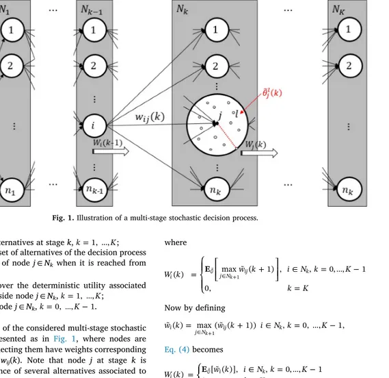
wij(k): deterministic utility of node j ∈ Nkwhen it is reached from node i N ,k 1 k=1, …,K;•
˜ ( )jl k : random oscillation over the deterministic utility associatedwith alternative l ∈ Lj(k) inside node j ∈ Nk, =k 1,…,K;
•
Wj(k): expected utility of node j ∈ Nk, =k 0,…,K 1.Then, the general structure of the considered multi-stage stochastic decision process can be represented as in Fig. 1, where nodes are layered in stages and arcs connecting them have weights corresponding to the deterministic utilities wij(k). Note that node j at stage k is zoomed-in to show the existence of several alternatives associated to utilities within a certain radius of stochasticity. Moreover, since each alternative l has an utility affected not only by its dispersion in the node
j but also by the incomplete knowledge of the decision-maker, a further
oscillation ˜ ( )jl k can be considered for each alternative l. Finally,
ex-pected utilities of the future stages Wj(k) are represented as large white arrows at node j.
Given the above interpretation, the deterministic approximation approach proposed in[48]can be applied to our problem. Please note that, in that work, the authors called “mutually exclusive alternatives” the nodes of our problem, while our different alternatives inside each node were called “scenarios”.
4.1.2. Toward a mathematical formulation
Letw k˜ ( )ij be the random utility of node j ∈ Nkwhen it is reached from nodei Nk 1,k=1, ,…K. Since we assume an efficiency-based
process (seeSection 3.3), the decision-maker would choose, among the different alternatives l ∈ Lj(k), the one which maximizes the random choice utility, i.e.,
= + + = + + = … w k w k k W k w k k W k i N j N k K ˜ ( ) max ( ( ) ˜ ( ) ( )) ( ) max ˜ ( ) ( ), , , 1, , . ij l L k ij j l j ij l L k j l j k k ( ) ( ) 1 j j (1) Now, by defining = = … k k j N k K ˜ ( )j max ˜ ( ), , 1, , , l L k j l k ( ) j (2) one obtains = + + = … w k˜ ( )ij w kij( ) ˜ ( )j k W kj( ), i Nk 1,j N kk, 1, ,K (3) where = + = … = + W k w k i N k K k K E ( ) max ˜ ( 1) , , 0, , 1 0, i ˜ j Nk 1 ij k (4) Now by defining = + = … + w k˜ ( )i max ( ˜ (w k 1)) i N k, 0, ,K 1, j Nk 1 ij k (5) Eq. (4)becomes = = … = W k w k i N k K k K E ( ) [ ˜ ( )], , 0, , 1 0, i ˜ i k (6) The recursive formula(3)shows that the random utility of node
j ∈ Nk, when it is reached from i N ,k 1 is composed of a deterministic utility wij(k), a random utility oscillation ˜ ( ),j k and an expected utility of the future selected nodes Wj(k). In such a way the random utilities w k˜ ( )ij become nested over stages. In the terminology of Dynamic Pro-gramming, node i Nk 1is a state and selecting node j ∈ Nkis a po-tential action, given that state i already chosen at the previous stage. At each stage, a node is chosen given the current state in a stochastic process having the Markov property. In our setting the value function is defined by W(k), which is computed in(6)as a Bellman equation[8]. It should be noted that, differently from other paradigms for modeling multi-stage optimization problems under uncertainty (e.g., Stochastic Programming or Stochastic Dynamic Programming), in our case we assume that the uncertainty of random oscillations is not revealed over the process. Such a recursive formula allows to determine the total utility of an optimal path without identifying the path (i.e., the se-quence of decisions) itself.
Because of the nested structure of the decision process, the max-imum expected total utility of the whole multi-stage stochastic decision process will be = =
[
]
= W W(0) E max ˜ (1)w E [ ˜ (0)].w j N j 0 ˜ 0 ˜ 0 1 (7)Therefore, the optimal path problem (in its maximization case) in a multi-stage stochastic decision network can be formulated as follows
=
[
]
W E max ˜ (1)w x j N j j ˜ 0 01 1 (8) subject to= = … + + x x 0 h N k, 1, ,K 1 i N ihk j N hjk 1 k k 1 k 1 (9) = = … x 1 k 1, ,K i N j N ijk k 1 k (10) = … xijk {0, 1} i N ,j N k, 1, ,K k 1 k (11)
wherexijkare Boolean variables taking value 1 if node j is selected at stage k after node i N ,k 1 k=1,…, ,K and 0 otherwise. The objective function(8)expresses the expected value of the maximum total utility of the whole multi-stage stochastic decision process. Please note, in fact, that all the other variablesxijkare embedded into the variablesx01j of the objective function. Constraint(9)ensure that the computed result is indeed a path between a source and a designated destination passing through stages. Constraint(10) indicates that at each stage only one decision (choosing the next node) is taken. Finally, binary conditions on the variables are stated in(11).
4.2. Minimization approach
As already stated, the optimization model for the minimization case (shortest path) can be easily obtained by using the same above proce-dure but with the following precautions
•
all the utilities, namely, the deterministic ones wij(k), their oscilla-tions˜ ( ),jl k and the expected utilities Wj(k), must be interpreted as costs. This means that W becomes the expected total cost of the decision process•
max must be substituted by min inEqs. (1),(2), (4), (5), (7), and(8).5. Deterministic approximation
According to the model formulation above, inSection 5.1we will derive in detail a deterministic approximation for the longest/most-profitable path value (maximization approach). Simple precautions to apply the same framework to obtain an approximation for the shortest path value (minimization approach) are given in Section 5.2. In Section 5.3, we provide a way to derive a feasible solution for both the optimization perspectives while, inSection 5.4, we briefly discuss the large applicability of the approximation approach.
5.1. Maximization approach
Since we want to provide an approximation of the maximum total utility, let us first consider just the objective function(8). In that case, i.e., without any path constraint involved, the problem has the fol-lowing trivial solution
= = x 1, if ˜ (0)w max ˜ (1)w j N 0, otherwise . j j q N q 01 0 0 1 1 (12) Now, by defining = w˜ (0) max ˜ (1)w q N q 0 0 1 (13)
and because of(12), the objective function(8)becomes
=
W E [ ˜ (0)].{ ˜}w0 (14)
Please note that the value of W in(14)cannot be calculated ana-lytically since we do not have precise information on the distribution of the random oscillations jl( )k. Let us call the probability distribution of
k ( ) j l as = = … F x( ) Pr{ ˜ ( )lj k x}, j N lk, L k kj( ), 1, ,K (15)
and the cumulative right distribution function ofw k˜ ( )i as
= = …
G x ki( , ) Pr w k{ ˜ ( )i x}, i N kk, 0, ,K 1. (16)
Then, we can use the following theorem.
Theorem 1.[48]Let us assume that
•
the random oscillations jl( )k are independent and identicallydis-tributed (i.i.d) random variables;
•
F(x) has an asymptotic negative exponential behavior in its righttail, i.e., > + = + F x y F y e 0 | lim 1 ( ) 1 ( ) . y x (17) Then, = = = … + G x ki( , ) lim G x k L( , | |) exp( A k e( ) ), i N k, 0, ,K 1 L i i x k | | (18) where β > 0 is a parameter to be calibrated,
= + + + + = … + A ki( ) (k 1)e , i N k, 0, ,K 1 j N j [w k( 1) W k( 1)] k k ij j 1 (19) is the accessibility in the sense of[22]to the overall set of nodes at stage (k+1), and αij(k) is the ratio
= = …
k l k l k j N k K
( ) ( )/ ( ), , 1, ,
j j k (20)
which remains constant for each pair (j, k) while the number of alter-natives do increase.
Theorem 1states that the probability distribution Gi(x, k) can be asymptotically approximated by a double-exponential (Gumbel) dis-tribution. So, when the total number of alternatives of the decision process becomes very large, the expected value of the maximum total utility(14)can be approximated by
= +
W 1/ (lnA0(0) ) (21)
where γ ≃ 0.5772 is the Euler constant, and
= + A (0) (1)e j N j w W 0 [ ij(1) j(1)] 1 (22)
is the accessibility to the set of nodes at stage 1.
5.2. Minimization approach
In case of the shortest path problem (minimization instead of maximization), similar theoretical results can be obtained by assuming
•
F(x) is the survival function of the probability distribution of˜ ( ),jl ki.e.,(15)becomes
= > = …
F x( ) Pr{ ˜ ( )lj k x}, j N lk, L k kj( ), 0, ,K (23)
•
F(x) has an asymptotic exponential behavior in its left tail, i.e.,(17) becomes + = > F x y F y e lim 1 ( ) 1 ( ) , 0. y x (24) Considering the above assumptions, the final equations equivalent to(21)and(22), but in the minimization approach, are= + W 1/ (lnA0(0) ) (25) and = + A (0) (1)e j N j w W 0 [ij(1) j(1)] 1 (26) respectively.
5.3. Finding a feasible solution
It is important to highlight that the expected value calculated in (21) represents just an approximation of the expected value of the maximum total utility. As already stated, the approximation is obtained by following the recursive formula in(3)that somehow also embeds the creation of a sequence of nodes, one selected at each stage. However, given the nature of the approximation, it is clear that the above se-quence of nodes could not satisfy the path constraints(9)–(11).
Therefore, the creation of a feasible solution for the problem (besides the approximation of its objective function) is still an open issue, which we address in the following way. Let us first recall a theorem, which holds under the same conditions discussed forTheorem 1inSection 5.1.
Theorem 2.[48]The probability pij(k) for choosing node j at stage k after node i at stage k 1 is given by
= + + = … p k l k e l k e i N j N k K ( ) ( ) ( ) , , , 1, , ij j v k W k q N q v k W k k k [ ( ) ( )] [ ( ) ( )] 1 ij j k iq q (27) which represents a Nested Multinomial Logit model.
Theorem 2defines a model for the continuous probabilities of the choices and does not address the construction of a feasible path made by one single node per stage. However, let us consider a graph in a multi-stage structure, where to each arc (i, j) at stage k a weight equal to the probability pij(k) (as defined in (27)) is assigned. By finding a longest path on that graph, an approximated optimal path solution over stages can be then determined. The rationale behind this choice is to look for the most probable sequence of nodes which satisfies constraints (9)–(11). We will also discuss the quality of this approach through various experiments inSection 6.
5.4. Applicability of the approximation
In this section, we want to highlight the quite large applicability of the proposed approximation. Even if condition in(17)yet represents a mild assumption on the shape of the distribution of the stochastic variables, Fadda et al.[15]have recently proved thatTheorem 1still holds when(17)is relaxed to the following condition
> + = + B x a exp 0 | lim ( ) L k L k L k e | ( ) | | ( )| | ( )| x (28) where B(x) is the probability distribution of ˜ ( ),j k i.e.,
= = …
B x k( , ) Pr{ ˜ ( )j k x}, j N kk, 1, ,K (29)
and a|L(k)|is chosen equal to the root of the equation =
B x L k
1 ( ) 1
| ( )|. (30)
Assumption(28)is equivalent to ask that the unknown distribution of the stochastic maximum utility ˜ ( )j k belongs to the domain of at-traction of a Gumbel distribution. This new result further enlarges the applicability of the approximation approach, which theoretically holds for any distribution of the form1 e p x( )where p(x) is a polynomial
function, such as the Normal, the Gumbel, the Weibull, the Logistic, the Laplace, the Lognormal, and many others.
It is easy to see that the new condition is milder, since assumption in (17)implies assumption in(28), while the converse is not true (e.g., the Normal distribution does not satisfy(17)).
6. Computational results
In this section, we present the results of the computational experi-ments carried out with the aim of evaluating the effectiveness of the deterministic approximation approach to find the solution and value of optimal path in stochastic multi-stage networks. The evaluation is performed by considering the expected value problem, in which the random variables are replaced by their expected values, and comparing its optimum value with that of the proposed approach. The determi-nistic approximation has been coded using MATLAB version R2016b, while the expected value problem has been implemented in GAMS 24.5.6. All the computational tests have been performed on an Intel(R) Core(TM) Processor i5 6200U (CPU 2.30 GHz) with 16 GB RAM.
Our experiments are focused on the longest path problem, i.e., they exactly reflect the maximization approach presented in Section 5.1. More precisely, inSection 6.1we describe the instances set generated as a testbed for our assessment. The calibration of β parameter is presented inSection 6.2, while the results of our computational experiment are described and commented inSection 6.3.
6.1. Instance sets
To evaluate the performance of the proposed approximation approach, we randomly generated networks with| |Nk ={5, 10, 20, 50, 100} nodes per stage k=1, …,K. Without loss of generality, we assume
= = …
Nk N k, 1, ,Kwhich indicates the nodes associated to each Nk re-present the entire set of nodes for the decision process at hand. This means that we can consider the same set of nodes at each decision stage and, in order to make sure to take into account all possible paths in the network, the number of stages K will be equal to the number of nodes (which is the same at each stage). In all the experiments, 100 alternatives for each node
= …
j N kk, 1, , ,K have been considered, i.e.,| ( )|L kj =100.
The utility observations associated to choosing alternative l inside node j coming from node i,i Nk 1,j N lk, L k kj( ), =1,…, ,K are
generated according to the Uniform, Normal, and Gumbel distributions in the range [1, δ], with = {50, 100, 150}. The parameter δ simply al-lows us to control the behavior of the approximation against different magnitude of utilities. The deterministic utility wij(k) is calculated as a mean value of the utility observations over the alternatives. For each one of the possible 45 combinations of number of nodes per stage |Nk|, δ value, and the three distribution types (Uniform, Normal, and Gumbel), we generated 10 random instances, which results in 450 instances in total. Note that, in generating observations using the Gumbel and Normal distributions, the location parameter =µ /2 is used. For the Gumbel distribution, a proportional scale parameter =0.5µ is adopted. As suggested in[34], the scale factor has been chosen experimentally so that the 98% of the probability lies in the considered truncated domain [1, δ] for each possible instance. Similarly, for the Normal distribution, the standard deviation = /6 is set so to give a 99% confidence interval.
The three above distributions, besides being very common in many practical applications, have been chosen to represent quite extreme cases of possible unknown distributions of observations to test throughout our experiments. In fact, the Gumbel distribution theoretically represents the best case to be approximated, whereas the Uniform distribution does not even satisfy the assumptions needed to derive the approximation. The Normal distribution is somehow in between the two extremes, satisfying assumption(28)but not satisfying(17). A final remark is necessary to justify the use of the Uniform distribution in our tests, for which the theoretical framework does not hold. In fact, in practical applications, it is often the case that a set of observed scenarios are available, but it is not
possible to derive a precise or even partial knowledge in terms of their probability distribution. Therefore, the experiments with the Uniform distribution can give us insights on whether the approach results accu-rate and robust even against unknown distributed scenarios which may not satisfy our approximation assumptions.
6.2. Calibration of parameter β
The effectiveness of deterministic approximation is mainly depen-dent on an appropriate value of the positive parameter β. This para-meter describes the dispersion of preferences among the different choice alternatives at each stage of the decision making process. Taking into account the concept of the expected utility of node j at stage k, parameter β is computed in a way that Wj(k) should be equal to the maximum utility that can be achieved by choosing the next node and then an alternative inside it at stage +k 1. Since, depending on the current node and stage, the possible maximum utility in the next stage is different, a parameter βikshould be calculated for any node i at any stage k by using
= + = = …
W ki( ) 1/ik(lnA ki( ) ) wimax( ),k i N kk, 0, ,K 1. (31) Here, wimax( )k represents the maximum utility that can be achieved by
making decision at stage +k 1,i.e.,
= + + + + + = … + wi ( )k max (w k( 1) ¯ (k 1) W k( 1)), i N k, 0, ,K 1 j N ij j j k max k 1 (32) where¯ (j k+1)is the average value of random oscillation utilities over the alternatives inside node j, i.e.,
+ = + + = … = + + k k L k j N k K ¯ ( 1) ( 1) | ( 1)|, , 0, , 1. j l L k j l j k 1 ( 1) 1 j (33) In our case, since we take the deterministic term of utility wij(k) as the average value of observations over alternatives, it is possible to collapse stages into a single one (containing all the possible alter-natives) and to find just one β parameter value which works for the entire network (in line withTheorem 1). More precisely, let us consider only one decision making stage which contains all nodes of the network and assign to each of them a new utility weight w j N¯ ,j ,computed as a mean value of deterministic utility wij(k), i.e.,
= = w w k K N j N ¯ ( ) ·| |, . j k K i N ij 1 k 1 (34)
Hence, the unique value of parameter β is calculated such that the ex-pected utility of the decision making process (i.e., choosing one of these nodes) equals the maximum utility that can be achieved, i.e.,
+ =
ln A w
1/ ( ( 0(0) )) max (35)
The left hand side ofEq. (35)represents the expected utility W, A0(0) is the accessibility to all the nodes with new weights, and wmaxis the maximum utility that can be achieved by choosing a node in a one-stage decision making process and is computed as
= +
w max( ¯w ¯ )
j N j j
max
(36) in which ¯jis the average value of random oscillation utilities over al-ternatives inside node j in all stages, i.e.,
= = = k K L k j N ¯ ( ) ·| ( )|, . j k K l L k j l j 1 1 ( ) j (37) Please note that this calibration approach is somewhat general and, therefore, can be used with any available dataset. The experiments reported inSection 6.3over random generated instances will show a
good confidence on this calibration method.
6.3. Computational results
In this section, we summarize and discuss the results obtained from our experiments on all the instance sets generated as discussed in Section 6.1and using the β value calibrated as presented inSection 6.2. The results contain two main distinct parts. The first one aims to assess the accuracy of the deterministic approximation of the maximum total utility W, while the second part evaluates the quality of the optimal path solutions derived by calculating an optimal path of a probability weighted network as described inSection 4.
For both maximum total utility and path solutions, the results of the approximation approach are compared with the Expected Value Problem (EVP) considered as a benchmark. In the expected value pro-blem, the weight of each arc is considered as the expected value over observations. Since the experiments are performed for the maximiza-tion approach, the benchmark path solumaximiza-tion is derived by finding the longest/most-profitable path in the network. The performance, in terms of percentage gap, is evaluated through the calculation of the Relative Percentage Error (RPE) as follows
= ×
RPE W opt
opt
: EVP 100
EVP
where W and optEVPrepresent the optimum of the deterministic ap-proximation (see Eq. (21)) and the optimum of the expected value problem, respectively.
Tables 1–3present the RPE associated to the instances generated by using the Uniform, Normal, and Gumbel distributions, respectively. Each entry of these tables reports statistics of the RPE over 10 random generated instances, given a specific combination of values of |Nk| and
δ. In particular, the tables show the average, the best, the worst RPE,
and its standard deviation (columns RPEavg, RPEbest, RPEworst, and RPEσ, respectively).
The first thing that should be noticed is that, as expected, the average RPE increase as the size of network grows for the three dis-tributions with the worst case of 1.30, 1.40, and 2.45 in 100-node network (average over δ values) for the Gumbel, Normal and Uniform
Table 1
RPE of the maximum total utility between the deterministic approximation and expected value problem for the Uniform distribution.
Instance RPE(%)
|Nk| δ RPEavg RPEbest RPEworst RPEσ
5 50 0.97 0.02 2.44 0.75 5 100 1.25 0.18 2.25 0.67 5 150 1.30 0.14 2.30 0.79 avg: 1.17 0.12 2.33 0.74 10 50 1.33 0.21 2.18 0.68 10 100 1.38 0.14 2.15 0.62 10 150 1.40 0.35 2.69 0.68 avg: 1.37 0.24 2.34 0.66 20 50 1.37 0.54 2.20 0.49 20 100 1.41 0.74 2.07 0.46 20 150 1.47 0.86 2.23 0.40 avg: 1.41 0.71 2.17 0.45 50 50 1.99 1.44 2.32 0.26 50 100 2.06 1.56 2.71 0.37 50 150 2.16 1.54 2.56 0.30 avg: 2.07 1.51 2.53 0.31 100 50 2.41 2.09 2.74 0.19 100 100 2.43 2.19 2.77 0.19 100 150 2.52 2.22 2.80 0.21 avg: 2.45 2.17 2.77 0.20 global avg: 1.69 0.95 2.42 0.47
distributions, respectively. Other trends can be noticed, by looking at the average RPE for various values of δ. It seems that smaller intervals give better results of approximation for the three distributions and across all the sizes. It means the approximation approach behaves better with smaller dispersion and magnitude of the realizations. The best RPEs also follow the same described behavior with little dis-continuities, while the worst ones have more fluctuations for all the combinations of different network sizes and distributions. Taking into account the standard deviation RPEs, it can be seen that the values are very similar together, i.e., less than 0.5% in global average, which de-notes a good stability in terms of variance.
Comparing the results for the three distributions highlights better performance, as expected, of the Normal and Gumbel distribution with
respect to the Uniform distribution for all considered sizes and dis-persions in terms of the average, best, worst, and standard deviation RPE.
We now want to assess the quality of the path solutions obtained by using the Nested Multinomial Logit (NML) model explained in Section 4. We again use as performance indicator the RPE, modified as follows
= ×
RPE opt opt
opt
: NML EVP 100
EVP
where optNML represents the value of the feasible solution obtained through the application of the NML model. Table 4 reports RPE averages and standard deviations for the three distributions. The results show promising performance of the Nested Multinomial Logit model for deriving optimal path solutions in terms of average and standard de-viation RPE which indicates a good performance and overall robustness of the approach. As it can be seen, the quality of the path solution is not dependent on the network size and the distribution.
Finally, despite of the quality obtained by the deterministic ap-proximation approach in terms of accuracy, we also want to point out its efficiency. The computational times for deriving the maximum total utility (tDA) and the path solution (tpath) are reported inTable 5. Since we have noticed that the computational times were somehow independent from the distribution used and the range of random generated utility weights, we just report average computational times for the various sizes of the network. First, note that finding the optimal path solutions needs just slightly more time compared to the de-terministic approximation calculation for larger-size instances. Moreover, not surprisingly, the time increases as the size of the net-work increases. The CPU time is in particular affected by the curse of dimensionality due to the recursive formula in (3). However, con-sidering the difficulty to solve the underlying problem under un-certainty for a suitable number of scenarios, the approximation ap-proach shows reasonably small CPU times. Few seconds are needed for networks with up to 20 stages and 20 nodes per stage, while about 10 minutes are needed for networks with up to 100 stages and 100 nodes per stage. This gives the possibility to embed the approximation into most sophisticated optimization algorithms for multi-stage problems under uncertainty.
7. Conclusions
In this paper, we have used a quite efficient and accurate approach to estimate the value and the structure of optimal paths in a multi-stage stochastic decision network. In this network decisions are made under uncertainty and the oscillations of the stochastic parameters follow an unknown probability distribution. The optimal path is seen as a se-quential decision making over stages, where the uncertain utility of nodes at each stage is affected by both previous and next decisions. By using some results from[48], we have determined a deterministic ap-proximation for the longest path value. Moreover, a feasible solution is obtained by heuristically using a Nested Multinomial Logit model, which gives the probability to optimally choose each node. Numerical tests, on a great number of random generated networks, have shown accurate estimations with respect to analogous results obtainable from solving the expected value problem. The performance of our determi-nistic approximation seems particularly good as the size of networks increase, making the proposed approach a valuable tool to support decision-making in stochastic multi-stage networks for large and com-plex applications.
Future works could consider the use of the given deterministic ap-proximation in different and more specific operational management problems involving multi-stage stochastic decision processes. For ex-ample, some multi-periodic applications in the home health-care field (see, e.g.,[33]) seem appropriate to be studied under this perspective.
Table 2
RPE of the maximum total utility between the deterministic approximation and expected value problem for the Normal distribution.
Instance RPE(%)
|Nk| δ RPEavg RPEbest RPEworst RPEσ
5 50 0.57 0.11 1.36 0.41 5 100 0.69 0.05 1.78 0.53 5 150 0.79 0.25 2.00 0.61 avg: 0.69 0.14 1.71 0.52 10 50 0.54 0.02 1.31 0.50 10 100 0.60 0.14 1.01 0.25 10 150 0.68 0.34 1.03 0.24 avg: 0.61 0.16 1.12 0.33 20 50 0.65 0.14 1.14 0.29 20 100 0.92 0.20 1.53 0.40 20 150 0.99 0.42 1.70 0.37 avg: 0.85 0.25 1.45 0.35 50 50 1.01 0.84 1.29 0.14 50 100 1.29 0.83 1.78 0.30 50 150 1.34 0.88 1.72 0.25 avg: 1.21 0.85 1.60 0.23 100 50 1.38 1.02 1.59 0.21 100 100 1.39 1.14 1.72 0.22 100 150 1.44 1.15 1.81 0.25 avg: 1.40 1.10 1.70 0.22 global avg: 0.95 0.50 1.51 0.33 Table 3
RPE of the maximum total utility between the deterministic approximation and expected value problem for the Gumbel distribution.
Instance RPE(%)
|Nk| δ RPEavg RPEbest RPEworst RPEσ
5 50 0.43 0.08 1.06 0.36 5 100 0.48 0.13 1.30 0.35 5 150 0.70 0.03 1.55 0.55 avg: 0.53 0.08 1.30 0.42 10 50 0.62 0.01 1.45 0.44 10 100 0.76 0.09 1.63 0.42 10 150 0.79 0.33 1.68 0.43 avg: 0.72 0.14 1.59 0.43 20 50 0.68 0.18 1.33 0.39 20 100 0.79 0.40 1.24 0.26 20 150 0.86 0.31 1.27 0.31 avg: 0.77 0.29 1.28 0.32 50 50 0.98 0.06 1.85 0.66 50 100 1.01 0.67 1.35 0.19 50 150 1.13 0.88 1.40 0.19 avg: 1.04 0.54 1.53 0.35 100 50 1.22 0.95 1.46 0.15 100 100 1.33 1.05 1.60 0.17 100 150 1.36 1.20 1.58 0.13 avg: 1.30 1.07 1.55 0.15 global avg: 0.87 0.42 1.45 0.33
Finally, from a more methodological point of view, one might embed this approach into a shifting-window framework that considers a re-stricted horizon in an iterative way, in order to mitigate the approx-imation errors in finding optimal paths over stages.
Conflict of interest
The authors have no conflict of interest.
References
[1] Akamatsu T. Cyclic flows, markov process and stochastic traffic assignment. Transp Res Part B 1996;30:369–86.
[2] Albareda-Sambola M, Fernandez E, Laporte G. The dynamic multi-period vehicle routing problem with probabilistic information. Comput Oper Res 2014;48:31–9. [3] Angelelli E, Bianchessi N, Mansini R, Speranza MG. Short term strategies for a
dy-namic multi period routing problem. Transp Res Part C 2009;17:106–19. [4] Angelelli E, Mansini R, Vindigni M. The stochastic and dynamic traveling purchaser
problem. Transp Sci 2016;50.https://doi.org/10.1287/trsc.2015.0627. [5] Archetti C, Jabali O, Speranza MG. Multi-period vehicle routing problem with due
dates. Comput Oper Res 2015;61:122–34.
[6] Baillon J, Cominetti R. Markovian traffic equilibrium. Math Program. 2008;111(1-2):36–56.
[7] Baringo L, Conejo AJ. Risk-constrained multi-stage wind power investment. IEEE Trans. Power Syst. 2013;28:401–11.
[8] Bellman R. Dynamic programming. 1957.
[9] Ben-Akiva M, Lerman SR. Disaggregate travel and mobility choice models and measures of accessibility. In: Hensher D, Stopher P, editors. Behavioral travel modeling. London: Croom Helm; 1979.
[10] Ben-Akiva M, Lerman SR. Discrete choice analysis: theory and application to travel demand. 9. MIT Press; 1985.
[11] Castro PM, Harjunkoski I, Grossmann IE. Rolling-horizon algorithm for scheduling under time-dependent utility pricing and availability. Comput Aided Chem Eng 2010;28:1171–6.
[12] Cheng TCE, Kuo WH, Yang DL. Scheduling with a position-weighted learning effect based on sum-of-logarithm-processing-times and job position. Inf Sci
2013;221:490–500.
[13] Demirel E, Demirel N, Gokcen H. A mixed integer linear programming model to optimize reverse logistics activities of end-of-life vehicles in Turkey. J Clean Prod 2016;112:2101–13.
[14] Domencich T, McFadden D. (1975). Urban travel dynamics: a behavioral analysis. North Holland, Amsterdam.
[15] Fadda E, Fotio Tiotsop L, Manerba D, Tadei R. The stochastic multi-path traveling salesman problem with dependent random travel costs. Technical Report (DAUIN-ORO-2019-01) Dept. of Control and Computer Engineering, Politecnico di Torino. 2019. http://www.orgroup.polito.it/material/DAUIN-ORO-2019-01.pdf
[16] Fosgerau M, Frejinger E, Karlstrom A. A link based network route choice model with unrestricted choice set. Transp Res Part B 2013;56:70–80.
[17] Galambos J. The asymptotic theory of extreme order statistics. New York: John Wiley; 1978.
[18] Gawiejnowicz S. Time-dependent scheduling. Springer-Verlag, Berlin; 2008. [19] Gendreau M, Ghiani G, Guerriero E. Time-dependent routing problems. Comput
Oper Res 2015;64:189–97.
[20] Glensk B, Madlener R. Multi-period portfolio optimization of power generation assets. J Oper Res Decis 2013;23:21–38.
[21] Govindan K, Fattahi M, Keyvanshokooh E. Supply chain network design under uncertainty: a comprehensive review and future research directions. Eur J Oper Res 2017;263:108–41.
[22] Hansen W. How accessibility shapes land use. J Am Inst Plan 1959;25:73–6. [23] Hartmann S, Briskorn D. A survey of variants and extensions of the
resource-con-strained project scheduling problem. Eur J Oper Res 2010;207:1–14.
[24] Hsu CJ, Ji M, Guo JY, Yang DL. Unrelated parallel-machine scheduling problems with aging effects and deteriorating maintenance activities. Inf Sci 2013;253:163–9. [25] John ST, Sridharan R, Ram Kumar P. Multi-period reverse logistics network design
with emission cost. Int J Logist Manag 2017;28:127–49.
[26] Kelley JE. Critical-path planning and scheduling: mathematical basis. Oper Res 1961;9:296–320.
[27] Kolm PN, Tütüncü R, Fabozzi FJ. 60 years of portfolio optimization: practical challenges and current trends. Eur J Oper Res 2014;234:356–71.
[28] Lee WC, Wu CC, Hsu PH. A single-machine learning effect scheduling problem with release times. Omega 2010;38:3–11.
[29] Leonardi G. The structure of random utility models in the light of the asymptotic theory of extremes. In: Florian M, editor. Transportation planning models. Elsevier; 1984. p. 107–33.
[30] Leonardi G. Asymptotic approximations of the assignment model with stochastic heterogeneity in the matching utilities. Environ Plan A 1985;17:1303–14. [31] Liu L, Wang JJ, Wang XY. Single machine due-window assignment scheduling with
resource-dependent processing times to minimize total resource consumption cost. Int J Prod Res 2016;54:1186–95.
[32] Luce RD. Individual choice behavior: a theoretical analysis. New York: John Wiley; 1959.
[33] Manerba D, Mansini R. The nurse routing problem with workload constraints and incompatible services. IFAC-PapersOnLine 2016;49:1192–7.
[34] Manerba D, Mansini R, Perboli G. The capacitated supplier selection problem with total quantity discount policy and activation costs under uncertainty. Int J Prod Econ 2018;198:119–32.
[35] Manerba D, Mansini R, Riera-Ledesma J. The traveling purchaser problem and its variants. Eur J Oper Res 2017;259:1–18.
[36] Marley A. Random utility models and their applications: recent developments. Math
Table 4
RPE of the optimal path between the approximation approach and expected value problem for the Uniform, Normal and Gumbel distribution.
Instance Uniform distribution Normal distribution Gumbel distribution
|Nk| δ RPEavg RPEσ RPEavg RPEσ RPEavg RPEσ
5 50 0.13 0.09 0.05 0.08 0.06 0.10 5 100 0.05 0.09 0.06 0.12 0.05 0.03 5 150 0.08 0.06 0.06 0.11 0.07 0.06 avg: 0.09 0.08 0.06 0.10 0.06 0.06 10 50 0.12 0.04 0.05 0.12 0.06 0.06 10 100 0.07 0.07 0.03 0.04 0.05 0.10 10 150 0.11 0.12 0.04 0.03 0.04 0.05 avg: 0.10 0.08 0.04 0.06 0.05 0.07 20 50 0.04 0.02 0.05 0.07 0.06 0.10 20 100 0.08 0.07 0.03 0.04 0.04 0.04 20 150 0.05 0.06 0.04 0.05 0.03 0.02 avg: 0.05 0.05 0.04 0.05 0.05 0.06 50 50 0.05 0.05 0.04 0.07 0.05 0.07 50 100 0.04 0.03 0.05 0.05 0.03 0.04 50 150 0.04 0.05 0.05 0.06 0.04 0.05 avg: 0.04 0.04 0.05 0.06 0.04 0.05 100 50 0.06 0.04 0.04 0.04 0.04 0.04 100 100 0.04 0.03 0.03 0.03 0.05 0.04 100 150 0.05 0.03 0.04 0.03 0.03 0.03 avg: 0.05 0.03 0.03 0.03 0.04 0.04 global avg: 0.06 0.05 0.04 0.06 0.04 0.05 Table 5
Computational time in seconds for calculating the deterministic ap-proximation and path solutions.
Nk tDA(s) tpath( )s 5 0.36 0.39 10 1.68 1.71 20 8.20 8.25 50 120 132 100 900 997
Soc Sci 2002;43:289–302.
[37] Moon JY, Shin K, Park J. Optimization of production scheduling with time-de-pendent and machine-detime-de-pendent electricity cost for industrial energy efficiency. Int J Adv Manuf Technol 2013;68:523–35.
[38] Mosca. Integrated transportation-inventory models: a review. Oper Res Perspect 2019;6:1–12.
[39] Nickel S, Saldanha da Gama F, Ziegler HP. A multi-stage stochastic supply network design problem with financial decisions and risk management. Omega
2012;40:511–24.
[40] Niu H, Zhou X. Optimizing urban rail timetable under time-dependent demand and oversaturated conditions. Transp Res Part C 2013;36:212–30.
[41] Ozceylan E, Paksoy T. Interactive fuzzy programming approaches to the strategic and tactical planning of a closed-loop supply chain under uncertainty. Int J Prod Res 2014;52:2363–87.
[42] Pasandideh SHR, Akhavan-Niaki ST, Asadi K. Bi-objective optimization of a multi-product multi-period three-echelon supply chain problem under uncertain en-vironments: NSGA-II and NRGA. Inf Sci 2015;292:57–74.
[43] Perboli G, Tadei R, Baldi M. The stochastic generalized bin packing problem. Discret Appl Math 2012;160:1291–7.
[44] Perboli G, Tadei R, Gobbato L. The multi-handler knapsack problem under un-certainty. Eur J Oper Res 2014;236:1000–7.
[45] Pillac V, Gendreau M, Gueret C, Medaglia AL. A review of dynamic vehicle routing problems. Eur J Oper Res 2013;225:1–11.
[46] Soleimani H, Seyyed-Esfahani M, Akbarpour-Shirazi M. Designing and planning a
multi-echelon multi-period multi-product closed-loop supply chain utilizing genetic algorithm. Int J Adv Manuf Technol 2013;68:917–31.
[47] Tadei R, Perboli G, Manerba D. A recent approach to derive the multinomial logit model for choice probability. In: Daniele P, Scrimali L, editors. New trends in emerging complex real life problems. AIRO Springer Series book series (AIROSS, 1). 2018. ODS2018, sept 10-13, 2018. Taormina (Italy)
[48] Tadei R, Perboli G, Manerba D. The multi-stage dynamic stochastic decision process with unknown distribution of the random utilities. Optim Lett 2019.https://doi. org/10.1007/s11590-019-01412-1.
[49] Tadei R, Ricciardi N, Perboli G. The stochastic p-median problem with unknown cost probability distribution. Oper Res Lett 2009;37:135–41.
[50] Toriello A, Haskell WB, Poremba M. A dynamic traveling salesman problem with stochastic arc costs. Oper Res 2014;62:1107–25.
[51] Wang JB, Sun LY. Single-machine group scheduling with linearly decreasing time-dependent setup times and job processing times. Int J Adv Manuf Technol 2010;49:765–72.
[52] Wei CM, Wang JB, Ji P. Single-machine scheduling with time-and-resource-de-pendent processing times. Appl Math Model 2012;36:792–8.
[53] Wen M, Cordeau JF, Laporte G, Larsen J. The dynamic multi-period vehicle routing problem. Comput Oper Res 2010;37:1615–23.
[54] Zeballos LJ, Mendez CA, Barbosa-Povoa AP, Novais AQ. Multi-period design and planning of closed-loop supply chains with uncertain supply and demand. Comput Chem Eng 2014;66:151–64.