The ground deformations: tools, methods and application to some Italian volcanic regions

(1)

Università degli Studi di Salerno

Facoltà di Scienze

Matematiche, Fisiche e Naturali

Dipartimento di Fisica “E. R. Caianiello”

Dottorato di Ricerca in Fisica

X Ciclo, 2° Serie (2008-2011)

The ground deformations: tools, methods and

application to some Italian volcanic regions

Coordinator: Prof. Giuseppe Grella

Tutor: Prof. Roberto Scarpa

(2)

(3)

3

Abstract

The objective of this thesis is the study of slow deformation of the soil as a result of intrusion of magma inside the magmatic chambers of some volcanoes located in Southern Italy. In particular, the Mt. Vesuvius and Campi Flegrei caldera have been monitored over the last 7 years. The research has been accomplished through the use of geodetic instrumentation (long baseline tiltmeters, Sacks-Evertson dilatometers) that has been installed during the entire period of the research near the aforementioned volcanoes. The data were recorded with the aid of data-logger, some of which are specifically designed for the current research.

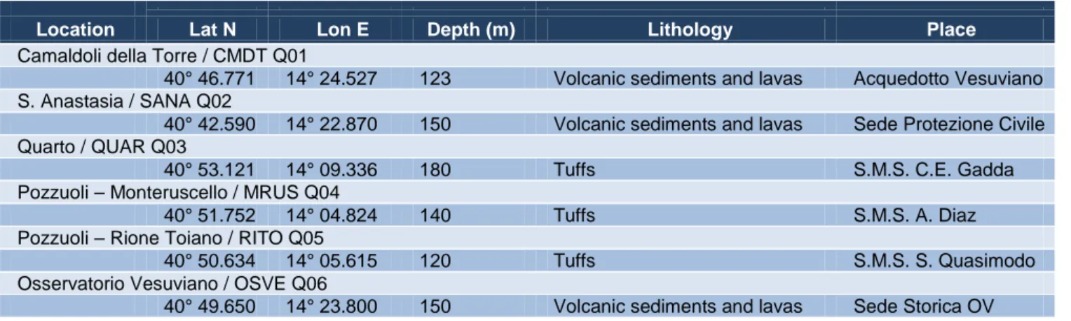
Campi Flegrei and Mt. Vesuvius are two volcanoes located near Naples, already monitored by Osservatorio Vesuviano, the local office of INGV (Istituto Nazionale di Geofisica e Vulcanologia). In the last 40 years systematic recordings of seismic data, of changes in distance of milestones, of leveling lines, of local gravimetric anomalies and of GPS-InSAR data have been carried out. Starting from 2004, the monitoring network maintained by Osservatorio Vesuviano has been enriched by the DINEV project: this is intended as a complementary network of geodetic stations and consists in the installation of a small array of 6 borehole stations (with an average depth of 120 m), each of which is constituted by a three components borehole broadband seismometer Teledyne Geotech KS2000BH and a Sacks-Evertson areal strainmeter (dilatometer). In addition, two three components surface broadband seismometers Guralp CMG 3-ESP have been installed to control the anthropogenic surface noise.

In Campi Flegrei caldera, then, another array of instruments has been installed: two long baseline water tiltmeters have been installed in Italian Army abandoned tunnels. The total length of tiltmeters is about 350 m for the northernmost tunnel, and of about 150 m for the southernmost tunnel. Tiltmeters were installed, respectively, in axial and tangential direction in respect with the position of the Campi Flegrei magmatic chamber.

The use of the instruments described in the current report allows to model the strain field in the range of low frequencies, monitoring the deformation tensor for its non-diagonal components (pure tilt) by using the tiltmeters, and the diagonal components (pure deformation) by using the dilatometers.

The monitoring is occurred for a time range of some years in length, needed to remove the seasonal drifts due to changes in rainfalls, while the deformation due to changes in barometric pressure have been deleted using linear regression techniques.

(6)

(7)

7

Chapter 1 – Introduction

Seismic and volcanic processes are usually associated to catastrophes and other kind of destructive phenomena, but, from a geophysical and geological point of view, they represent even the only signals Earth gives us in order to allow scientists to understand the complex dynamics that still regulate the changes in our young planet.

The internal structure of the Earth can, so, be understood by an inverse analysis that starts from these phenomena: following the strategies developed by geophysicists it is, in fact, ideally possible to learn what the Earth contains in its depths and, hopefully, one day predict the next catastrophic event.

The study of the Earth’s internal structure is performed by using a huge range of different instruments, each of them recording a different kind of signal.

Seismic waves have been constantly monitored, recorded and analyzed in the past decades, allowing scientists to better understand how the Earth’s interior is layered, and all the theoretical studies performed over the data recorded by the seismic networks available all over the World gave us a more precise idea of Earth’s internal structure, how seismic waves travel in the depths and on surfaces which separate the different layers, and the kind and entity of damages they could do to human artifacts. Seismic waves transport high frequency energy, which can be easily monitored through the usage of a wide range of different seismometers (accelerometers, velocity transducers and so on).

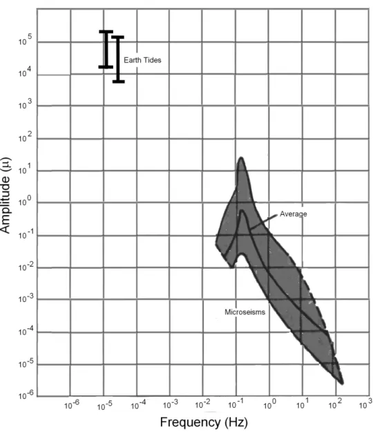
The spectrum of the energies emitted by the Earth, anyway, has a wide series of different values, ranging from the very high frequencies of body waves, to the very low frequencies of the secular strain, as represented in Table 1-1. In this context, seismology and geodesy represent the two extremes for geophysicists. Seismology can be seen as the branch of geophysics which studies the phenomena related with the high frequency energy emission due to earthquakes, strong motion events, volcanic eruptions and so on. Geodesy, on the other hand, is the branch of geophysics related with the study of emission of energy at lower frequency: Earth tides, tectonic plates subduction, aseismic deformations, magmatic chambers pressure changes, crustal deformation are all examples of low frequency phenomena which are described by the geodesy.

(8)

8

Table 1-1 – Frequency ranges vs. geophysical phenomena

Frequency range Phenomenon

10-8÷10-7 Hz Secular strain

10-6÷10-4 Hz Tides

10-5÷10-1 Hz Afterslip – Slow ruptures

10-3÷10-2 Hz Dynamic fault rupture

10-3÷103 Hz Body waves propagation

Lower frequency doesn’t mean lesser energy: usually low frequency waves transport even higher energies than the most destructive earthquake, even if in the former case energies are averaged on a longer time than the latter case.

Geodetic phenomena are related with deep changes of the Earth’s interior: the monitoring of these events can be used to verify the Earth’s response to gravitational interaction with celestial bodies (Sun-Moon system interaction which generates the Earth tides) and the plate tectonic theory, and even to predict possible volcanic eruptions through the analysis of strain and tilt data near large volcanic calderas.

The following PhD thesis is about the development of an integrated network of instruments which are used to record and analyze deformation data coming from the Campi Flegrei-Mt. Vesuvius volcanic region, located in the southern part of the Italian peninsula. The instrument network deployed by University of Salerno, with international scientific partners (Carnegie Institution of Washington, Washington D.C. and University of Colorado, Denver), consists of areal strainmeters and tiltmeters, associated with broad-band seismometers and barometric pressure transducers.

During the years 2004-2005 an array of 6 borehole areal strainmeters (dilatometers) was installed in the region, in order to record strain tensor diagonal components. To improve the recording quality, barometric pressure was also taken in account, recording it at the same sampling frequency of the strain, and thereafter removed from the raw strain trends: since the dilatometers output can in principle be expressed as a linear combination of areal strain and vertical strain due to barometric changes, the strain changes due to the atmospheric pressure can be modeled just as an uniaxial stress or strain (or more rigorously as distributed loads applied to the surface of a half-space, to a layer of distinct elastic properties overlying the half-space, or to the surface of a spherical earth).

(9)

9

The six dilatometers were installed in boreholes separated each other by several kilometers, and the so developed network was chosen to cover critical distances from the crustal magma bodies which underlie beneath the Campi Flegrei and Vesuvius volcanoes.

In order to further improve the network, each station was integrated with a three-component broad-band accelerometer, to avoid the strain field changes due to high frequency seismic waves and to calibrate the dilatometers in the high frequency range.

During the years 2007-2008, moreover, near the Campi Flegrei caldera were installed two long baseline water-filled tiltmeters: tilt components (i.e., the components not lying on the diagonals) of the strain tensor can be monitored through the data recorded by tiltmeters.

The complete network of instruments can, so, be used to monitor all the strain tensor components.

1.1 – Strainmeters and Dilatometers

Stresses and strains have long been of great importance in various human activities. Engineers are used to use small devices, known as strain gauges, in which the resistance of a metal wire or semiconductive film varies with strain. In the past, these devices where tried to be used even by geophysicist in order to measure rock stress: the results were poor, because of their insensibility. Geophysicists, then, started to design their own strainmeters.

Most of the geophysical strainmeters are extensometers, measuring the displacement between two separated points. Extensometers may usefully be divided into three classes according to what they use to span the distance between endpoints: rod strainmeters (some used in boreholes), wire strainmeters and optical strainmeters. A final class of strainmeters uses hydraulic amplification to make borehole measurements: the best known example of this class of strainmeters, which is even the instrument used in the following of the current report, is the Sacks-Evertson areal dilatometer.

1.1.1 – Rod Strainmeters

The very first rod strainmeter ever built for seismometry, was produced by Benioff in early 1930s. This instrument consists of a 20m iron pipe attached at one end to a pier and at the other to a variable reluctance transducer, which drove a recording galvanometer. Using a solid rod to transfer the relative displacement of one point to another has the merit of extreme simplicity: for all but the highest frequencies the rod may be treated as a rigid body, and the frequency response is flat. Typically it was used as active element a velocity transducer, which made the instrument a strain rate gauge, which is desirable for seismic recording because it reduces the noise from temperature fluctuations and tides. Many different rod strainmeters have been developed during time, by only changing the rod material and the way in which the displacements between rod and piers are measured.

Many rod strainmeters were built so that they were able to measure tidal and secular strains, whose typical frequencies are completely ignored by seismometers due to their own design.

(10)

10

Because the displacements measured by mechanical rod strainmeters are very small, an accurate calibration is difficult. Benioff applied a force to the free end of the strainmeter rod and used its known elasticity to convert this to a displacement. Another calibration method usually followed, is to mount the fixed part of the sensor on a motion reducer driven by a micrometer. Lately, interferometers have also been used for calibration of rod strainmeters and to record their long-term motion.

In the most recent period, borehole extensometers have been deployed too. Because of the advantages of a borehole instrument, both in flexibility of deployment and possible long-term stability, several miniature rod extensometers have been built for borehole installations. In all of these the ends of extensometer are attached to a thin canister that is cemented to the borehole wall. Because the base-length is short, the displacements to be detected are small, and they are usually measured with capacitance sensors. Moore et al. [1974] designed a borehole strainmeter that used a 0.14m quarts-rod length standard. At high frequencies the nominal noise was -230dB relative to 1𝜀2

𝐻𝑧. The only installation reported was made in a

1.5m deep borehole drilled in a mine tunnel: the strainmeter recorded tides adequately and showed an exponentially decreasing drift (about 10-13 s-1 after 200 days) presumably from cement expansion.

1.1.2 – Wire Strainmeters

Although several rigid-rod strainmeters have been designed to be portable, this has never been practical because the length standard is so cumbersome. As a more convenient alternative, several designs have instead used a flexible wire. Because a wire must be supported by keeping it in tension, which increases creep, this might seem unwise, but in fact wire strainmeters have been very successful, especially for tidal measurements. The earliest design hung an Invar wire between two points in a shallow catenary; changes in the distance between the ends caused the bottom of the catenary to rise and fall. This motion was recorded with an optical lever. More recent instruments stem from the design by Sydenham [1969] of a strainmeter in which the wire is fixed at one end and at the other is free to move but kept under constant tension.

The design of such an instrument is governed by the theory of a flexible line suspended in a catenary. The usual development [Bomdford, 1962] gives the relation between base-length l, wire length w, and central sag y as

𝑤 = 𝐿𝐶𝑠𝑖𝑛ℎ �_𝐿𝑙

𝐶� (1.1.1)

𝑦 =1_{2 𝐿}𝐶�𝑐𝑜𝑠ℎ �_𝐿𝑙

𝐶� − 1� (1.1.2)

where the catenary scaling length LC is _𝜌𝑔𝐴2𝐹0

𝑤, ρ being the density of the wire and Aw its cross-sectional area. F0 is the tension at the lowest point; for a shallow catenary this is very near the tension at the end. This

(11)

11

𝐿𝐶 = 2𝑒𝑤_{𝜌𝑔 ≡ 𝑒}𝐸 𝑤𝐿𝑤 (1.1.3)

where E is the Young’s modulus of the material and we have defined a wire scaling length 𝐿_𝑤=2𝐸

𝜌𝑔. For a

given material, Lw is fixed and while it is desirable to make LC large to keep the catenary flat, this entails

increasing ew, which should be kept small to minimize creep.

Because the length standard is flexible, wire strainmeters have many spurious resonances at relatively low frequencies [Bilham and King, 1971]. One mode is longitudinal oscillation of the wire and tensioning system. Tension is usually applied by a weight on a lever; in a longitudinal oscillation this act as a mass and the wire as a spring. The frequency of oscillation fl depends on the moment of inertia of the tensioning

system (Ip), the distance from the pivot point to the attachment point of the wire (ra), and the effective spring

constant of the wire, which acts as it had a Young’s modulus of 𝐸

𝑊. The result is

𝑓𝑙=_{2𝜋 �}𝑟𝑎 𝐴_𝐼𝑤𝐸 𝑃𝑊�

1_�₂

. (1.1.4)

The wire can also oscillate transversely, with the restoring force being some combination of tension and gravity. The gravest purely tensional mode has a frequency of

𝑓𝑡=1_{𝑙 �}𝑔𝐿𝑤_{8 �}𝑒𝑤 1_�₂

. (1.1.5)

It is relatively easy to make these frequencies a few hertz (above the microseism band), but difficult to make them much larger: wire strainmeters are poor seismometers.

1.1.3 – Laser Strainmeters

Because the wavelength of light, unlike any material object, is an invariant standard, interferometry has obvious attractions for strain measurements. The development of the laser, with its very long coherence length, made it possible to build extensometers using interferometers with very unequal arms. Though several groups have built laser strainmeters, only a few designs have produced significant results. Among the others, here should be mentioned the laser strainmeter produced by the University of California, San Diego (UCSD) [Berger and Lovberg, 1970], the instrument from Cambridge University [Goulty et al., 1974] and one from the U.S. National Bureau Of Standards (NBS) [Levine and Hall, 1972]. All of the hundreds of other laser strainmeters are evolution of the design of the above mentioned instruments, which will be used in the following of the current paragraph as a reference.

The USCD strainmeter used the most straightforward optical design: an unequal-arm Michelson interferometer, in which changes in the length of the long arm cause fringe shifts at the detector. Counting fringes gives the strain change, with the frequency response and dynamic range being limited by the counting electronics. Using suitable optics, a change of 𝜆 4� can be detected in the path length difference Λ:

(12)

12

since the path length is twice the instrument base-length l, this corresponds to a strain of 𝜆 8𝑙� . While the optics are relatively simple, l must be fairly large to get adequate resolution. For the UCSD instrument, l is 731m, giving a least count of 0.108 nε. This length means that the instrument has to be located above ground, in fact, building an instrument that could be so installed was a goal of this design, since such a surface installation allows a wider choice of sites than one in mines and tunnels.

Figure 1.1 – Mechanical design of the UCSD laser strainmeter. The two endpoints are tall piers of dimension stone sunk in the ground. These, and the optics they carry, are inside temperature-controlled enclosures in air-conditioned buildings. The measurement path is inside a vacuum pipe except at the very ends; telescopic joints keep the length of the air paths constant.

On the other hand, a surface installation complicates the mechanical design of the strainmeter (Figure 1.1). Almost all of the optical path along the long arm runs through a pipe evacuated to 1 Pa, so that temperature and pressure changes do not matter. For ease of adjustment the interferometer optics and remote retro-reflector are not in the vacuum. Because of this, any motion of the end of the evacuated pipe changes the proportion of the path in air and in vacuum, and therefore the optical path length, with 1mm of motion causing an apparent strain of 0.4 nε. Temperature changes cause the aluminum pipe to expand and contract up to 0.6 m. To eliminate this problem, the vacuum pipe is anchored in the middle, and telescopic joints are put at each end; these joints are servo-controlled to keep the end of the evacuated path a constant distance from the optics. A prism at the midpoint of the pipe allows a break in the optical path, so that the pipe need not be in a single straight section. The optics at each end are inside heavily-insulated boxes in small air-conditioned buildings In the three instruments first built the endpoints were long columns (up to 4 m) of dimension stone sunk into the ground, Because these tilted (causing spurious strains), the endpoints for the fourth instrument were short piers in vaults just below the surface. Displacements of these piers proved to be large enough [Wyatt, 1982] that optical anchors were needed to correct for them.

The optical system had lots of refinements, one of which was the isolation of the laser from the light returning through the beam-splitter, using a polarizer and quarter-wave plate. This is needed to keep the laser from “seeing” the modes of the optical cavity formed by the long interferometer arm, and having its frequency pulled towards them. Because of the length of the instrument, the laser beam must be expanded before being sent into the vacuum pipe, to reduce diffractive spreading.

(13)

13

The interferometer is illuminated by a single-frequency laser whose wavelength is stabilized by locking it to a reference cavity: it is formed by two mirrors, separated by a 30cm quartz spacer and kept in a tightly controlled environment. The mirrors form a Fabry-Perot interferometer [Born and Wolf, 1980] in which there is a multiple interference of the light that bounces back and forth between the two ends. If the mirrors transmit slightly so that light can be sent in one end, the ratio of intensity coming out the other to that sent in is 𝐼𝑇 𝐼𝑙 = �1 + 4𝐹𝑛2 𝜋2 𝑠𝑖𝑛2� 4𝜋Λ𝑐 𝜆 �� −1 (1.1.6)

where λ is the wavelength of the light, Λc is the optical path length between the ends (including phase shifts

at the mirrors), and Fn the finesse (optical Q) of the system, which depends on the reflectivity and alignment

of the mirrors. Even for highly reflective mirrors, the system is transparent for Λ_𝑐 =𝑁𝜆

2 (N an integer) and

transmits less well for other values of λ; for Fn large the transmittance falls rapidly as λ shifts away from one

of the resonant values. About the instrument described here, the value of Λc is fixed and the laser light

transmitted through it is measured by a photo-detector. Because Fn is about 100, small shifts in λ cause a

large change in the intensity received. The signal from the photo-detector changes the size of the laser cavity to maximize this intensity.

In this paragraph it has been stressed out the design of the USCD laser-strainmeter since huge similitude there exist with the tiltmeters used in the following of the current report.

1.1.4 – Borehole Hydraulic Strainmeters

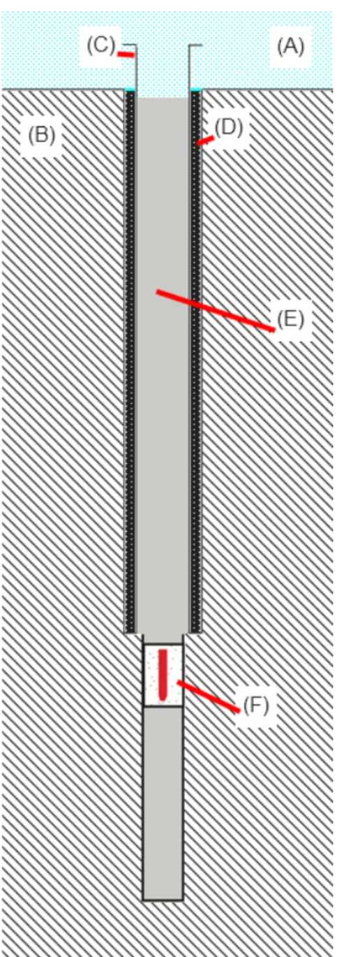
In his first strainmeter paper, Benioff [1935] suggested that dilatational strains might be measured by burying a large container of liquid with a small opening. Strains in the ground would change the volume of the container and force liquid to flow in and out; for a sufficiently small opening the flow could be detected. Benioff’s idea does not seem to have been tried until 30 years later, when it was revived by Sacks and Evertson. Their very first design has seen wide use, especially in Japan [Suyehiro, 1982]; the most complete description of it is in the thesis written by Evertson [1977]. The basic principle is the same as that suggested by Benioff, with the sensing volume (Figure 1.2) cylindrical so that it fits in a borehole. The outer case is divided into two parts: the actual sensing volume, completely filled with liquid, and a smaller backing volume, partly filled with inert gas. Changes in the size of the sensing volume force liquid in and out of the backing volume, which offers little resistance because of the high compressibility of the gas. The liquid actually flows into and out of a bellows inside the backing volume, and the bellows motion is measured. The two volumes are also connected by a valve; if the sensing volume changes so much that the bellows would be pushed past its limits, opening this valve equalizes the pressure in the two volumes and re-zeroes the bellows. The tube connecting the sensing volume to the bellows attenuates high-frequency motions, protecting the bellows from large, rapid changes, such as those expected near an earthquake.

(14)

14

Figure 1.2 – Simplified cross-section through a Sacks-Evertson dilatometer, shown cemented in a borehole. The sensing volume S is largely filled by a hollow insert and has a filling port at the bottom. The only openings between the sensing volume (lower) and the backing volume (upper) are the re-zero valve V (shown open) and the capillary to the bellows B. A DC-LVDT L above the bellows measures the bellows motion

The response of the hydraulic system depends not only on the relative size of the volumes but also on the compressibility of the liquid in the sensing volume and on the stiffness of the bellows. If the bellows is much smaller than the sensing volume, we may assume the liquid in the bellows to be incompressible. The sensing volume is

𝑣𝑠= 𝑣𝑠0(1 + 𝐷) (1.1.7)

where D is the dilatation of the instrument. The bellows volume is

𝑣𝑏= 𝑣𝑏0+ 𝐴𝑏𝑞 (1.1.8)

where Ab is the effective area of the bellows and q the displacement of its end; this linear approximation is

very accurate for well-made bellows [Scaife et al., 1977]. By conservation of mass we find

� 𝑝 1 + 𝑝𝑠 𝑘𝑠 � � 𝑣𝑠 0_{(1 + 𝐷) + 𝜌(𝑣} 𝑏0+ 𝐴𝑏𝑞) = 𝜌(𝑣𝑠0+ 𝑣𝑏0) (1.1.9)

where ρ is the density of the liquid, ks its bulk modulus, and ps the pressure in the sensing volume, which is

(15)

15 𝑝𝑠 =𝑘_𝐴𝑏𝑞

𝑏 +

128𝜂𝐿𝑡𝐴𝑏

𝜋𝑏𝑡4 𝑞̇ (1.1.10)

where the first term comes from the pressure produced by the bellows, which has a spring rate kb, and the

second term comes from the pressure drop along the connecting tube, assuming laminar flow. Lt is the tube

length, bt its diameter, and η the dynamic viscosity of the liquid. Making the approximation that ps << ks,

these two equations can be combined to give

𝑞 �1 +𝑘_𝐴𝑏𝑣𝑠0 𝑏 2_𝑘 𝑠� + 𝑞̇ � 128𝜂𝐿𝑡𝑣𝑠0 𝜋𝑏𝑡4𝑘𝑠 � = − 𝑣𝑠0 𝐴𝑏𝐷. (1.1.11)

At long periods the effect of liquid compressibility is thus to reduce the instrument response from the “ideal” �−𝑣𝑠0 𝐴𝑏� by a factor 𝐾𝐻= �1 +𝑘𝑏𝑣𝑠 0 𝐴_𝑏2_𝑘 𝑠� −1 . (1.1.12)

At high frequencies the connecting tube attenuates the response, acting as a single-pole low pass filter with a corner frequency of 𝑓𝑐= 𝑏𝑡 4_𝑘 𝑠 256𝐾𝐻𝜂𝐿𝑡𝑣𝑠0 . (1.1.13)

In the instruments put in Japan, vs 0

was 0.033 m3 and Ab 2 cm 2

, giving an ideal response of q = 170D, so that the displacements to be measured were roughly the same as for a 170m extensometer. However, the liquid used (silicone oil) was relatively compressible (ks = 9 × 108 Pa), and the bellows relatively stiff (kb =

970 N m-1, though in fact 85% of this came from the stiffness of a piezoelectric displacement transducer), so that KH was 0.51, reducing the effective “length” to 85m. Because the liquid had a relatively high

viscosity (0.019 N s m-2), it was not difficult to make bt small enough for fc to be about 1 Hz.

In the early instruments [Sacks et al., 1971] an inductive sensor measured the long-term bellows motion; in more recent versions, an LVDT is used for this, and the piezoelectric transducer has been eliminated. Another change has been done to reduce the volume of liquid by filling most of the sensing volume with a solid insert, usually a sealed hollow tube. This changes the apparent bulk modulus ks from that of the liquid,

kL, to 𝑘𝐿

�𝜒𝐿+(1−𝜒𝐿)𝑘𝐿_𝑘𝑙� where kl is the bulk modulus of the insert and

χL the fraction of νs 0

occupied by liquid. Instruments recently installed in California have had vs

0 = 0.028 m3, Ab = 0.43 cm 2 , and kb = 230 N m -1 ; given the increased effective rigidity of the liquid, the effective length was 325 m. The size of the connecting tube has been enlarged to raise fc into a range near 10Hz.

The response of the instrument depends not only on the relation between q and ∆ but also on that between instrument deformation and earth strain. If the instrument were perfectly flexible, the equations for an empty borehole show that

(16)

16

𝐷 = �2 − 𝜈_{1 − 𝜈� Δ} (1.1.14)

where ∆ is the volumetric strain in the absence of a hole and ν the Poisson’s ratio of the material. An approximate solution [Evertson, 1977] to the problem of an elastic tube cemented into a hole shows that the vertical strain is not altered and that for the tube used in the Sacks-Evertson instrument, the areal strain is 90% of what it would be in an empty hole, the above equation remaining about right.

The success of this strainmeter depends on careful attention to details. For example, any gas bubbles in the sensing volume would greatly decrease ks and reduce the response. To avoid this, the volume is filled

under vacuum, the silicone oil being distilled into it to remove volatile components. The installation must also be done carefully. Sack’s group places a slow-setting expansive cement of relatively low viscosity in the hole; the instrument is then lowered into this material, which sets around it, forming a tight pre-stressed bond.

While the Sacks-Evertson design is simple and robust, it cannot provide directional information. The borehole extensometers described above are one solution to this; another is a three-component hydraulic instrument developed by Sakata et al. [1982]. In this the sensing volume is almost completely filled by a solid cylinder, and the remaining annulus of liquid is divided into three sectors. The volume change of each sector is measured separately by a bellows and inductive displacement sensor, and the complete horizontal strain tensor is reconstructed form these three outputs.

1.2 – Inclinometers and Tiltmeters

Inclinometers and tiltmeters are instrument used by scientists to measure the inclination of a free surface (in our case, Earth’s ground surface), and, thus, to obtain a direct measure of the tilt components of the strain tensor (i.e., the pure rotational changes in a solid half-space).

The best long baseline tiltmeters allow geophysicists to obtain an angular resolution up to 10-9 rad over a period of the order of the day, and an annual drift that gives a stability of the order of 10-6 rad/year, which means that the maximum error on measures, in this case, is a mere 10-6 rad.

Just as for the case of strainmeters, there exist different kind of tiltmeters too. Short baseline inclinometers are the instruments usually used in seismic context, since are simple to be deployed on the field and easily manageable, but, on the other hand, they are not only very sensible to local inhomogeneities and anisotropies, but have even a lower resolution (typical values for short baseline tiltmeters is about 10-8 rad under ideal conditions, while somewhat smaller changes could be detected further lowering real resolution). The opposite extreme is represented by long baseline tiltmeters: the highest resolution is obtained through the use of an instrument hard to deploy, which needs a stable plain place, in stationary temperature conditions. In the current work, only long baseline tiltmeters will be taken in account.

(17)

17 1.2.1 – Long baseline tiltmeters

The first long baseline tiltmeters were built by Michelson in 1914. They are based on the communicating vessels physical principle, part of the Stevin’s law related to hydrostatic pressure: two jars were connected together by one pipe of about 15 m in length, half-filled with fluid. The instrument was placed 2 m beneath the Earth’s surface and closely tied to the ground, and the height changes in jars were measured by the use of a microscope. Differences in height of fluid’s surface in relation with the edge of jars at both ends of the pipe were related with a ground tilt deformation (solid rotation of the Earth’s free surface), which was consequently measured.

Tiltmeters can be installed both in deep tunnels or just on the Earth’s surface.

Deep tunnels (more than 100 m in depth) installations are primarily used in subsurface laboratories to study Earth tides or oceanic charge. In the case of deep tunnels installations, the rocks shield the thermal wave (in some cases thermal changes can be as low as 0.01° C/year) allowing resolutions up to 10-9 rad and stabilities up to 10-6 rad/year. Thanks to these features, the most stable tiltmeters can record free surface waves and Earth’s proper modes associated to the most energetic earthquakes.

Tiltmeters installed near the Earth’s surface (or just on it) have usually lower resolutions, due to the thermal effects produced by the dilatation of fluids used to built them [Beaven & Bilham, 1977]: changes in temperature of just 0.2° C on a 4 m tube half-filled of fluid with a slope of 2% can generate statistical errors up to 0.1 µrad. Statistical errors like this will not occur for horizontal pipes.

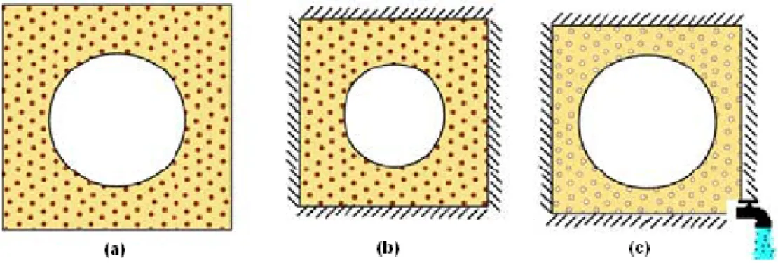
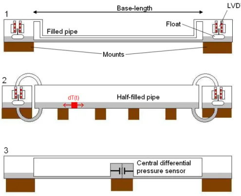
Different kind of tiltmeters can be installed, according to the type of transducer chosen to measure fluid surface changes: optical or laser interferometers, magnetic probes, floating devices or pressure measuring devices. According to the type of transducer and the geometry of the system jar / pipes, three different kind of tiltmeters can be distinguished: filled pipe with external floating devices, half-filled pipe with external floating devices and filled pipe with central pressure measuring device [Agnew, 1986]: in Figure 1.3 the three different kind of tiltmeters are shown and compared.

(18)

18

Figure 1.3 – Comparison between the different categories of long baseline inclinometers installed near the earth's surface

The first two kind of instruments are basically insensitive to uniform temperature variations since we look at the difference of level variations at the ends. Similarly, the third kind of instruments is insensitive to the same changes in temperature thanks to the central differential pressure sensor which will monitor changes in barometric pressure: uniform disturbances pose no problems indeed. This is also true for the problems of micro-leakage: the first two instruments shall be resistant to this type of problem, particularly the instrument no. 2 because it has a larger free surface of liquid. By cons, it must be more sensitive to the problems of evaporation.

It has been seen that the three instrument types are insensitive to uniform thermal perturbations. In opposition, if thermal changes occur locally on the pipes and supposing that all the pipes were put in places perfectly horizontally, only the third type of instruments (those with the central pressure sensor) will behave wrongly, and consequently will be perturbed: a fluid dilatation occurring in the left section of the instrument, in fact, will increase the height of the left section of the fluid’s free surface, causing a change in left section’s pressure on the central sensor, and this behavior will not re-equilibrate the fluid contained into the right section.

On the other hand, if the first kind of instrument was not installed correctly, presenting some ripples in its wall mounts (or support, depending on the type of installation), output will result in incorrect data when a local thermal perturbation occurs since fluid dilatation summed with pipe inclination generate a change in pressure gradient inside the fluid. Possible solution to this kind of problem are available and will be discussed in the following of the present work.

The second kind of instrument does not have this drawback because the expansion of the liquid due to local temperature changes affects uniformly the ends of the instrument. However, this type of installation

(19)

19

also requires a perfectly horizontal tube, and there are the same constraints for installation on site seen in the case of the first instrument. It seems that whatever is the type of instrument used, it is essential to have a horizontal line, which involves difficult installation in places where the topography is complex enough. The first two instruments are insensitive to tube deformation, while this is not the case for the third one. The instruments installed for this work use a floating device coupled with a displacement transducer which is used to measure the differential changes in height of the fluid free surface in order to obtain the tilt variation measured by the whole instrument, and its general design is very similar to the second instrument depicted into Figure 1.3.

1.2.2 – Precautions and limitations

One of the major problems for inclinometers is the stability of the supports which holds in place the instruments, particularly for short base inclinometers, but also for long baseline tiltmeters. These should minimally deform or move under the effect of local inhomogeneities in the risk of introducing instrumental drifts. It is therefore important to minimize the number of supports. Instruments 1 and 3 depicted into Figure 1.3 will be sensitive to vertical movements of the supports at the ends. The third instrument, in principle should be insensitive to local inclination of the central support.

In this case the second instrument depicted has higher benefits than the other two, since it could be installed with as low as 4 total supports, two placed to hold jars at both ends of the pipe, and two used to support the whole length of the pipe. This instrument is able to distinguish the movement of one of the jars over the other because of the large free surface of liquid in the tube half-filled, so it will be less sensitive to parasitic movements of the two jars. However, this instrument is sensitive to vertical movements of the supports at the ends of the tube half-filled. Finally it will be sensitive to the 4 support points.

Whichever the instrument installed, it is clear from this quick review of long baseline tiltmeters that it is of fundamental importance to be as much accurate as possible in installation of the instrument and in its coupling with the Earth’s surface.

1.2.3 – Previous long baseline tiltmeters installations

The largest installation in the world for a long baseline inclinometer station in surface was performed at Piñon Flat Observatory in California (USA).

In 1981, following the work of Bilham at the Seismological Observatory of Ogdenbourg in New York, the Lamont Doherty Earth Observatory developed an instrument with the record dimensions of 535 m in length, using the principle of measurement by laser interferometry [Bilham et al, 1979]. This instrument was installed at a depth of only 1 m.

Later, the University of UCSD also redeveloped the measuring principle of Michelson and Gale for the installation of an instrument of the same size with a measuring system which was using white light interferometry [Wyatt, 1982]. This instrument is placed next to the previous one, but uses different supports, and is formed by a half-filled pipe. The fluid used is a mixture of water and ethylene glycol to increase the

(20)

20

viscosity of the liquid which will better attenuate waves resonance on the free surface of the fluid flowing in the half-filled pipe. These waves can be excited by the presence of moderate earthquakes.

Finally, the University of Cambridge developed an instrument with the central pressure sensor of the same length of both previous tiltmeters [Horsfall & King, 1978]. This latter instrument is placed on the same supports as the Bilham’s instrument. Significant work has also been made to coupling both ends with the rock. The instruments are placed on pillars that are connected to stable points located at higher depths through invar bar extensometers using a magnetic transducer. In Figure 1.4 it is depicted a diagram similar to this type of system used in another installation in Mexico. The instrument developed by the UCSD uses a laser extensometer anchored at 26 m depth which can also check the stability of the pillars.

Figure 1.4 – Illustration of the method of coupling used at both ends of the half-filled pipe for the long baseline tiltmeters installed close Acapulco in the Mexican subduction zone.

(21)

21

Chapter 2 – Theory underlying Earth’s crust deformations

The theory underlying the Earth’s crust deformations derives from some different branches of the physics: the theory of continuum, the fluid dynamics, the theory of gravitation, the thermodynamics. Of course, to fully understand how sensors and other devices used in the following of the current work operate, other details need to be explained.

The current chapter deals with all of the theoretical information needed in order to better understand and appreciate the physics that governs deformations.

2.1 – Continuum mechanics: theory of elasticity

The theory of elasticity is one branch of continuum mechanics, which studies systems whose properties are defined at all points in space.

The two main elements to deal with in theory of elasticity are the stress – the force experienced at every point in space – and the strain – the displacement caused by stress. Other properties, such as temperature, could be of interest in some specific case (for example, thermal variations may contribute to overall rock deformations, and hence should be taken in account for a more accurate model).

In general, theory of elasticity tries to solve equations to find functions of the form 𝜑(𝑥, 𝑦, 𝑧; 𝑡), where x, y, z and optionally t are independent variables, whilst φ which could be a scalar of a vector, is a dependent variable.

2.1.1 – Stress tensor

Let’s consider an infinitesimal element of volume dV for a homogeneous body. It is subject to external body forces which act on each atom of the body. For the Earth’s interior, for example, these forces are the gravitational forces acting on the body as a whole. In addition to these forces, contact forces act on the external surfaces of the small volume too: these forces are produced by surrounding molecules through atomic or molecular interactions. An example of contact forces is represented by the pressure of a fluid

(22)

22

over a surface. The average contact force measured per unit area of a surface is known as stress (dimensionally, 𝑁 𝑚� 2= 𝑃𝑎).

Let’s now suppose to have an infinitesimal surface element dS having arbitrary orientation, and inside an homogeneous medium in static equilibrium, as depicted into Figure 2.1. The orientation of the small surface element can be specified through the use of the unit vector n, normal to the plane where dS lies. The force per unit area exerted through this surface by the molecules of the body on the side indicated by the direction of unit vector n is called traction and is represented by a vector 𝑻 = 𝑻 (𝒏), whose direction and magnitude depend on n.

Figure 2.1 – Explanation of the concept of traction

Obviously, in equilibrium the molecules present on the opposite side of dS exert a force 𝑻 (− 𝒏) = − 𝑻 (𝒏). The components of T normal and parallel to the plane of dS are called respectively normal stress and shear stress. In the case of a fluid shear stress is always zero, so we have: 𝑻 = − 𝑃𝒏, where P is the pressure.

Figure 2.2 - Three vectors of traction are sufficient to describe the surface forces acting in a point of the body: they act through three orthogonal surface elements in a Cartesian coordinate system xyz.

Now let’s consider the system of surface forces that are exerted at any point of the body. The resultant of these forces can be decomposed into three components, which are represented by tension vectors acting on three infinitesimal surfaces orthogonal and normal to the axes in the considered point (Figure 2.2).

(23)

23

Alternatively, by letting e1 ≡ x, e2 ≡ y and e3 ≡ z, where (x, y, z) are the unit vectors associated with the

Cartesian axes, we can describe the surface forces through a tensor of order 3. The stress tensor is the mathematical entity:

𝜏𝑖𝑗 = 𝑇𝑖�𝒆𝒋� (2.1.1)

In this notation the second index of the tensor indentifies the direction of the unit vector (i.e., the direction orthogonal to the surface), while the first index is the component of the traction vector. The stress tensor allows in turn to establish the traction exerted on any surface inside a body.

Figure 2.3 - Positive components of the stress tensor for four of the six faces of a cube.

From Figure 2.3 it is clear how tensor components are oriented into a system of Cartesian axes. For example, on the side identified by the unit vector e3, the element τ13 has a positive value when traction is

exerted along the e1 direction. Vice versa, on the opposite side – the one identified by the unit vector –e3 –

τ13, τ23 and τ33 assume a positive value when traction occurs, respectively, in direction –e1, –e2 and –e3,

since 𝑇_𝑖�−𝒆_𝒋� = −𝑇_𝑖�𝒆_𝒋�. This implies that:

𝜏𝑖𝑗= 𝜏𝑗𝑖 (2.1.2)

The equation (2.1.2) implies that the stress tensor is a symmetric tensor, since, for example, it is clear from Figure 2.3 that the couple generated by the components τ31 is opposed to the couple generated by the

components τ13. The equation (2.1.2), moreover, states another important property of the stress tensor:

only six of the total nine components of the tensor are independent. So, the stress tensor con be seen as the linear operator that generates a traction vector T starting from a directional unit vector n. Given any set of components τij, it is always possible to find a direction n for which there is no shear stress on a surface

(24)

24

𝑇(𝑛) = 𝜆𝑛 = 𝜏𝑛 (2.1.3)

where λ is a scalar. To find a direction n which satisfies (2.1.3) it must be solved, then, the following eigenvalue problem:

(𝝉 − 𝑰𝜆)𝒏 = 𝟎 (2.1.4)

where I is the identity matrix of order 3. This system of equations has a nontrivial solution only when:

det(𝝉 − 𝑰𝜆) = 0 (2.1.5)

The equation (2.1.5) is a third degree equation which admits three solutions, the eigenvalues λ1, λ2 and λ3.

Since τ is symmetric and real, the eigenvalues are real too. The three corresponding eigenvectors n(i) are orthogonal and define the principal axes of stress. To compute the components of the stress tensor in the principal axes system, in which the associated matrix has only diagonal nonzero components, we apply a simple transformation of similarity. The diagonalization of the stress tensor, hence, is:

𝝉′_{= 𝑵}𝑻_{𝝉𝑵 = �}𝜏1

′ ₀ ₀

0 𝜏2′ 0

0 0 𝜏3′

� (2.1.6)

where N is the matrix formed with the components of the three eigenvectors.

In the particular case in which it is τ’1 = τ’2 = τ’3, the stress field is called hydrostatic (in this case on the

small element of volume dV acts only the hydrostatic pressure) and there are no surfaces for which the shear stress is different from zero. In a fluid the stress tensor can be written as:

𝝉 = �−𝑃0 −𝑃0 00

0 0 −𝑃� (2.1.7)

where P is the pressure. Stress has units of force per unit area, as already stated at the beginning of the current paragraph.

(25)

25

Table 2-1 – Pressure variation with depth in the Earth

Depth (Km) Region Pressure (GPa)

0-24 Crust 0-0.6 24-400 Upper Mantle 0.6-13.4 400-670 Transition Zone 13.4-23.8 670-2891 Lower Mantle 23.8-135.8 2891-5150 Outer Core 135.8-328.9 5150-6371 Inner Core 328.9-363.9

Shear stress, conversely, is much smaller going deep, where it is associated with movements of mantle convection and with the propagation of seismic waves. A significant static shear stress is found only in the brittle upper crust (10-100 MPa).

2.1.2 – Strain tensor

Now let’s consider the problem of representing the deformation of a body subject to external forces. After a deformation, each point of the body, identified by a position vector 𝒓 = (𝑥₁, 𝑥₂, 𝑥₃), undergoes a shift u from its original position 𝒓_𝟎 = 𝒓 (𝑡₀) at the initial time 𝑡 = 𝑡₀.

Figure 2.4 – Geometry of deformation. The depicted example shows how deformation is associated to a relative shift du between two points that were originally separated by the distance dr.

The position taken by the points of the rigid-body system with respect to the starting positions can so be represented with a vector field, the displacement field u:

(26)

26

𝒖(𝒓𝟎) = 𝒓 − 𝒓𝟎 (2.1.8)

The displacement field gives an absolute measure of the changes in position of the points internal to a continuous body. Moreover, changes in position can occur even without deformations. This occur when |𝒓 − 𝒓′| is a constant for each couple of points r and r’.

Strain hence represents locally a measure of the relative variations of the displacement field, or rather of the spatial gradients of the field: for example, the extensional strain is defined as a change in length in respect to the original length of a body (e.g., a 100m long metal bar elongated up to 101m is subject to a displacement field which changes uniformly from zero to one meter along the bar, while the strain field is constantly equal to 0.01, or 1%).

Let’s now consider the displacement u for a point which originally was located in r, as depicted in Figure 2.4. It is possible to describe the displacement for a neighboring point, having initially position r + dr, by expanding u in Taylor series expansion, choosing a first order approximation. What we get is:

𝒖(𝒓 + 𝑑𝒓) = 𝒖(𝒓) + �_𝜕𝑥𝜕𝒖

𝑖𝑑𝑥𝑖 3

𝑖=1

. (2.1.9)

The relative displacement to the first order, so, is equal to:

𝑑𝒖 = �_𝜕𝑥𝜕𝒖

𝑖𝑑𝑥𝑖 3

𝑖=1

(2.1.10)

where the derivatives are computed in the point r.

The displacement can be divided into two different contributions: the deformation and the rigid rotation, which doesn’t contribute to the actual deformation. For this purpose, it is possible to decompose the matrix 𝐽𝑖𝑗 = 𝜕𝑢𝑖� in a symmetrical half and an anti-symmetrical half: _𝜕𝑥_𝑗

𝑱 = 𝜺 + 𝝎 (2.1.11)

where the symmetrical strain tensor 𝜀_𝑖𝑗= 𝜀_𝑗𝑖 has components:

𝜀𝑖𝑗 =1_{2 �}𝜕𝑢_𝜕𝑥𝑖 𝑗+

𝜕𝑢𝑗

𝜕𝑥𝑖� (2.1.12)

while the rigid-rotations tensor ω is anti-symmetrical (𝜔_𝑖𝑗 = −𝜔_𝑗𝑖) and has components:

(27)

27

The tensor ω describes a rigid-rotation of the body, but no deformations are associated with it. In fact, since ω is anti-symmetrical, the diagonal terms are all equal to zero, while, for the remaining six terms, there exist only three independent components. It is, hence, possible to form a vector Ω, with components:

Ω𝑘= �𝜀𝑖𝑗𝑘₂𝜔𝑖𝑗 3

𝑖𝑗=1

(2.1.14)

where εijk is the Levi-Civita tensor. Using the identity:

� 𝜀𝑖𝑗𝑘𝜀𝑠𝑡𝑘 3 𝑘=1 = � 𝜀𝑘𝑖𝑗𝜀𝑘𝑠𝑡 3 𝑘=1 = 𝛿𝑖𝑠𝛿𝑗𝑡− 𝛿𝑖𝑡𝛿𝑗𝑠 (2.1.15)

it is easy to prove that:

� 𝜀𝑖𝑗𝑘Ωk 3 𝑘=1 = � 𝜀𝑖𝑗𝑘𝜀𝑠𝑡𝑘₂ 𝜔𝑠𝑡 3 𝑠𝑡𝑘=1 =�𝜔𝑖𝑗− 𝜔₂ 𝑗𝑖�= 𝜔𝑖𝑗 (2.1.16)

and so it results that:

� 𝜔𝑖𝑗𝑑𝑥𝑗 3 𝑗=1 = � 𝜀𝑖𝑗𝑘Ωk𝑑𝑥𝑗 3 𝑗𝑘=1 = −(𝛀 × 𝑑𝒓)𝑖 (2.1.17)

This implies that the second term in equation (2.1.11) represents a rigid rotation around the Ω axes, so this term doesn’t imply any deformation.

On the other hand, the first term implies a net deformation, and it represents the Strain Tensor. All of its components are dimensionless and depend from the derivatives of the displacement field. These components are of two different types.

The diagonal components determine the way in which displacement along a coordinate axes varies along it: for example, if the displacement occurs only along the x1 direction (u2 = u3 = 0) and u1 changes only

along this specific direction, then the only term non-null of the strain tensor is ε11. If 𝜕𝑢𝑖 𝜕𝑥 𝑖

� > 0 then there is extension along the xi axes, while if 𝜕𝑢𝑖 𝜕𝑥

𝑖

� < 0 there is a contraction in length. If the diagonal term εii is

constant inside a rigid body that is deformed, it represents the change in length per unit length in xi

direction.

The generic non-diagonal terms in the strain tensor, however, represent the changes, along one axes, of the displacement along one different axes (for example, the changes of u1 when moving along the x3 axes).

Just as in the case of the stress tensor, even the strain tensor can be represented in a coordinate system where only the diagonal components are non-null. Let’s suppose that the displacements in a neighborhood

(28)

28

of a point r can be described by pure deformation (ω = 0). In this case the equation (2.1.10) can be re-written as:

𝑑𝒖 = 𝜺(𝒓)𝑑𝒓. (2.1.18)

The principal strain axes can then be calculated requiring that the variation of the displacement field du has the same direction of the change of position dr:

𝑑𝒖 = 𝜆𝑑𝒓 = 𝜺(𝒓)𝑑𝒓. (2.1.19)

The three eigenvalues of the equation (2.1.19) are known as principal strains ε1, ε2 and ε3. Apart the special

case in which ε1 = ε2 = ε3 (known as hydrostatic strain), an amount of shear strain is always present.

The trace of the strain tensor

Δ = � 𝜀𝑘𝑘 3 𝑘=1 = �𝜕𝑢_𝜕𝑥𝑘 𝑘 3 𝑘=1 = ∇ ∙ 𝒖 (2.1.20)

is called dilatation and is equal to the divergence of the displacement field 𝒖 = 𝒖(𝒓). Dilatation determines, as a consequence of a deformation, the change in volume per unit volume. In fact, into the principal strain axes system, a small element of the body with volume 𝑑𝑉 = 𝑑𝑥₁𝑑𝑥₂𝑑𝑥₃, becomes the volume:

𝑑𝑉′_{= �1 +}𝜕𝑢1 𝜕𝑥1� 𝑑𝑥1�1 + 𝜕𝑢2 𝜕𝑥2� 𝑑𝑥2�1 + 𝜕𝑢3 𝜕𝑥3� 𝑑𝑥3≅ �1 + � 𝜕𝑢𝑘 𝜕𝑥𝑘 3 𝑘=1 � 𝑑𝑥1𝑑𝑥2𝑑𝑥3= = �1 + �𝜕𝑢_𝜕𝑥𝑘 𝑘 3 𝑘=1 � 𝑑𝑉 = (1 + Δ)𝑑𝑉 (2.1.21)

Therefore the relative change in volume for the point in question is given by:

Δ =𝑑𝑉′− 𝑑𝑉

𝑑𝑉 (2.1.22)

and the rotor of the displacement field is: ∇ × 𝒖 = �𝜕𝑢3 𝜕𝑥2− 𝜕𝑢2 𝜕𝑥3� 𝒆𝟏+ � 𝜕𝑢1 𝜕𝑥3− 𝜕𝑢3 𝜕𝑥1� 𝒆𝟐+ � 𝜕𝑢2 𝜕𝑥1− 𝜕𝑢1 𝜕𝑥2� 𝒆𝟑. (2.1.23)

Comparing the equation (2.1.13) with the equation (2.1.23) shows that the rotor of the displacement field u is non-null only if ω is not identically null, or when a small amount of rigid rotation is present.

2.1.3 – Relationship stress-strain

In an elastic medium, stress and strain are related through a linear constitutive relationship whose more general form is:

(29)

29 𝜏𝑖𝑗 = � � 𝑐𝑖𝑗𝑘𝑙𝜀𝑘𝑙 3 𝑙=1 3 𝑘=1 (2.1.24)

The tensor cijkl is known as the elastic tensor, and the law (2.1.24) is known as Hooke’s Law for an elastic

medium. It assumes that the medium is perfectly elastic, so there is no energy loss or attenuation in response during deformation. The elastic tensor is a fourth order tensor with 81 (34) components. Remembering the symmetry of stress and strain tensors, and introducing some thermodynamic constraints, it can be shown that only 21 components are linearly independent. Moreover, usually the characteristics of a medium change with direction (anisotropic medium), while for isotropic mediums their features don’t depend from the chosen direction: using this constraint when referring to the Earth’s interior (a good first order approximation in many cases), the elastic tensor is invariant for rotations and the number of linearly independent parameters lowers to only two, related by the equation:

𝑐𝑖𝑗𝑘𝑙= 𝜆𝛿𝑖𝑗𝛿𝑘𝑙+ 𝜇�𝛿𝑖𝑙𝛿𝑗𝑘+ 𝛿𝑖𝑘𝛿𝑗𝑙� (2.1.25)

where λ and µ are known as Lamè parameters, while the δij is the Kronecker delta function. The Lamè

parameters are related with the propagation velocity of seismic waves. Using the equation (2.1.25), the Hooke’s law becomes:

𝜏𝑖𝑗 = 𝜆𝛿𝑖𝑗� 𝜀𝑘𝑘 3 𝑘=1

+ 2𝜇𝜀𝑖𝑗 = 𝜆𝛿𝑖𝑗Δ + 2𝜇𝜀𝑖𝑗 (2.1.26)

The Lamè parameters, hence, determine in a complete way the linear relationship between stress and strain in an isotropic medium. The parameter µ, particularly, is known as shear modulus and represent a measure of the resistance of the material to shear deformations. The parameter λ, on the other hand, doesn’t have a simple physical meaning.

Three more constants are used to describe the mechanical behavior of isotropic bodies: the Young modulus, the uniform compression modulus and the Poisson’s ratio.

The Young modulus E represents the ratio between extensional stress and the associated extensional deformation for a cylinder pulled from both sides. Its value is:

𝐸 =(3𝜆 + 2𝜇)𝜇_{𝜆 + 𝜇} (2.1.27)

The uniform compression modulus k gives a measure of how much incompressible a material is, and it is defined as the ratio between the applied hydrostatic pressure and the consequent volume change:

(30)

30

Finally, the Poisson’s ratio represents the ratio between lateral contraction of a cylinder pulled from both sides and its longitudinal extension:

𝜎 =_{2(𝜆 + 𝜇)}𝜆 (2.1.29)

Apart the dimensionless Poisson’s ratio, all of the other parameters are expressed in Pa.

2.2 – Definition and measure of the tilt

To define the slope of a given surface, we must define a reference frame in space. By definition a pendulum is naturally directed along the acceleration vector g, which defines the local vertical. We will therefore take as a vertical reference the same direction defined by the acceleration vector g. The direction of the two other components of the reference frame is perpendicular to the vertical, hence them define the horizontal surface: they lies therefore along a free surface of a liquid. Then, one possibility to measure the inclination of a surface is to identify the position of the free surface of a liquid relative to the surface. This is the fundamental principle of the hydrostatic long baseline inclinometer.

All inclinometers measure the change of angle a between the direction defined by the gravity and the normal to the Earth's surface where the inclinometer was installed. We therefore measure the variation of angle between the geoid, or the corresponding equipotential surface, and the base of the instrument. The change of inclination is measured in a reference frame defined by the geoid and vertical. The geoid defines the main horizontal directions x and y, while the acceleration vector g defines the vertical z [Horsfall 1977]. An long baseline inclinometer measures this slope along a base, that can range from a few meters to several hundred meters.

On a long baseline inclinometer, the variation of tilt angle between the base formed by the end-points and the geoid generates the movement of a portion of liquid from a pot to the other. This movement causes a variation in height of liquid positive in the first pot and negative in the second one. These variations in height, equal and opposite in sign at each end, are measured by sensors designed almost entirely of silica.

Figure 2.5 – Effects of the geoid and of the Earth’s crust deformation. In (1) it is represented the case without deformation: in this case the geoid surface (dashed line) is parallel with the fluid’s free surface. In (2) it is depicted the effect of tilt: in this case α represents the angle between the geoid surface (dashed line) and the fluid’s free surface (light blue plane), which acts as a horizontal reference.

(31)

31

The signal of interest coming from a hydrostatic inclinometer of length l is the subtraction of the two signals +h and –h. From these two values it is possible to establish the tilt of the crust in respect to the equipotential surface identified by the fluid’s free surface, starting from the equation:

tan 𝛼 =𝑑ℎ_{𝑙 =}�+ℎ − (−ℎ)�_𝑙 =2ℎ_{𝑙 ≅ 𝛼} (2.2.1)

The approximation reported in equation (2.2.1) is valid for small angles (as the case of crustal tilt deformations), while the angle α is represented in Figure 2.5.

The tilt and strain quantities are very similar [Agnew, 1986], and it is not easy to separate them: both are measures of deformation, even if inclination, however, introduces other effects. It establishes the general expression of the tilt vector ω = ωD + ωU (according to a purely kinematic description using the tensor

notation [Malvern, 1969], where ωD is the sum of the tilt deformations due to the elastic deformation of the

Earth, while ωU is the change of tilt produced by the lunisolar tidal potential, [d'Oreye, 2003]).

The final expression for ω is:

𝝎 = (𝒛𝟎∙ 𝒅𝟎)(𝒅𝟎∙ 𝜺) − 𝒅𝟎(𝒛𝟎∙ 𝒅𝟎∙ 𝜺)

+𝒛𝟎× (𝒅𝟎(𝒔 ∙ 𝒅𝟎) − 𝒔) −𝛁𝑼𝟏− 𝒛𝟎(𝒛𝟎∙ 𝛁𝑼_𝒈𝟏) + 𝒙̈ − 𝒛𝟎(𝒛𝟎∙ 𝒙̈)

(2.2.2)

This equation has five terms, two involving the strain tensor ε, one the rotation r, one the change of the lunisolar horizontal potential U1 and the last produced by the horizontal acceleration 𝒙̈. The slope will be

affected by all these terms. The vector s is defined below.

By adopting a fixed coordinate system, it is possible to propose a Lagrangian description of the relative position of two particles r(X1, t) and r’(X2, t) of an isotropic elastic rigid body. The distance between the two

particles is |𝑑𝒓|, as seen in Figure 2.4, while 𝒅_𝟎= 𝑑𝒓

|𝒓−𝒓′| is the unit vector directed along the dr direction.

Let’s now assume that the particle displacements are infinitesimal: they will form at time t the basis d, and |𝒖|

𝑙

� ≪ 1, it also requires that 𝑢 = 𝒓 ∙ 𝛁𝒖, this should be verified regardless of the direction of u, 𝛁𝒖 must be substantially constant for a distance l around the origin X1 of r. This condition implies that we have a

uniform strain tensor, even if in practice this is not always satisfied.

Starting from the definition of strain tensor ε stated in (2.1.12), and using the infinitesimal rotation vector:

𝒔 =1_{2 𝛁 × 𝒖} (2.2.3)

it is possible to choose as reference direction the unit vector z0 oriented along the local vertical defined from

(32)

32 𝒛𝟎=_|𝛁𝑼𝛁𝑼𝟎

𝟎| ≡

𝛁𝑼𝟎

𝒈 (2.2.4)

Under some specific conditions, the equation (2.2.2) can be simplified.

If T is the stress tensor, then on a free surface of a body, 𝒏 ∙ 𝑻 = 0, where n is the normal to the surface. This is the case when installing a device on the Earth’s surface. For an isotropic elastic material this implies that 𝒏 ∙ 𝜺 = 0, and if the normal in respect with the baseline on the free surface equals the generic unit vector, d0 = n, the inclination ωD produced by the deformation reduces to:

𝝎𝑫= 𝑧0× (𝒅𝟎(𝒓 ∙ 𝒅𝟎) − 𝒓) (2.2.5)

and the expression for ω becomes:

𝝎 = 𝒛𝟎× (𝒅𝟎(𝒓 ∙ 𝒅𝟎) − 𝒓) −𝛁𝑼𝟏− 𝒛𝟎(𝒛𝟎∙ 𝛁𝑼_𝒈𝟏) + 𝒙̈ − 𝒛𝟎(𝒛𝟎∙ 𝒙̈) (2.2.6)

An inclinometer placed on the free surface is subject to an inclination that is therefore only proportional to the rotation of the free surface, to horizontal variations of the lunisolar potential and to the local horizontal accelerations of the free surface. In the following of the current work, we won’t be interested in the horizontal acceleration component, since this term acts only when the inclinometer is subject to horizontal accelerations produced by seismic waves.

It is, then, possible to relate the equation (2.2.1) with the equation (2.2.6), in the following way: +ℎ − (−ℎ)

𝑙 = 𝜔 = 𝒛𝟎× (𝒅𝟎(𝒓 ∙ 𝒅𝟎) − 𝒓) −𝛁𝑼𝟏− 𝒛𝟎_𝒈(𝒛𝟎∙ 𝛁𝑼𝟏) (2.2.7) 2.2.1 – Units of measurement

The unit of measurement used in order to measure an angle variation is the degree (°).However, since the measures that we perform with our inclinometers have very small angle variations, a subunit of the degree is often used, it is the arcsecond as 1° = 60’ = 3600 a sec. Usually, the unit chosen to measure angle variations due to Earth’s crust deformations is the radians, since it can be quickly connected to the vertical deformation. For inclinometers, it belongs to the International System (IS). Arcsecond and radian can be easily connected: since 2π rad = 360°, we easily obtain that 1 rad = 206264.806247 a sec or 1 µrad = 206.264806247 ma sec.

There is no sign convention to determine in which way it is changing the tilt with an inclinometer. In usual installations, we always have two main directions: NS and EW directions. For the NS direction, so we have two possible directions, north or south, as well as EW, were there are the west and the east directions. For values of inclinations that will be presented in the following, every time we will state the direction of the tilt. For example when the inclinometer tilts NS positively to the north, it means that the N side subsides in respect to the S side.

(33)

33

2.3 – Tides-induced deformations

The combined effect of the gravitational interaction between Earth and other celestial bodies and the centrifugal force due to the revolution of Earth around the center of mass of the system consisting of the Earth itself and these celestial bodies, results in a viscoelastic deformation involving the lithosphere, hydrosphere and atmosphere. This deformation is known as tide: the largest contribution is provided by lunisolar attraction and features characters periodic or almost periodic: it is modulated in time as the Sun and Moon have different velocities and thus the combination of their distances from Earth is variable. The motion of the celestial bodies is described in an approximate geocentric system: although the mass of the Sun is much larger than the mass of the Moon, the attraction that it exerts on the Earth is about twice the solar attraction, since the Moon is closest to Earth. If we consider only lunar attraction, we would have only one major tide at the lunar zenith on a given meridian, but this won’t justify the reason why a swelling would be present at antipode. The previously appointed centrifugal force due to revolution of the Earth-Moon system is the cause of this deformation. Because of these forces, Earth changes its shape: these deformations are governed by the same laws of forces that cause them. The laws that govern these changes, other than instantaneous amplitudes, are calculated in the various components and with a high degree of accuracy, since are known the orbits of Earth and Moon and the values of their masses.

It is important to study tides, since this is the only deformation phenomenon for the Earth for which it is possible to calculate almost exactly the forces. Hence the study of Earth tides – the tides which concern the crust – is important for the determination of some physical properties of the Earth, and may have various applications in geophysics and geodynamics. It is aimed to know the components of the tidal field and their deviation from theoretical models: these deviations may be indicative of crustal deformation and mass redistribution in the subsurface. Thanks to these properties of the tidal signals, they can be used as a comparison for calibration of instruments.

2.3.1 – Tidal acceleration

Any point on the Earth’s surface is subject to four forces: • Gravitational attraction due to Earth’s own mass

• Centrifugal force due to Earth’s rotation around its own axis • Gravitational attraction due to other celestial bodies

• Centrifugal force due to the revolution of the system Earth-other celestial bodies around their common center of mass

The latter two forces define the tidal acceleration, which is responsible of tides.

Let’s consider now the generic two-bodies system (in our case, this is a good representation for the Earth-Sun or the Earth-Moon systems), as the one depicted into Figure 2.6.