PROJECT CL.E.A.R.
CLoudiness Experiment for Automatic Recognition C. Cornaro(2), S. Vergari(1), F. Foti(1), F. Del Frate(3)
(1)ReSMA - Centre of Meteorological Experimentations, via Braccianese Claudia Km 20.100, 00062 Bracciano, Italy. Tel. +39 06 9988 7701; Fax +39 06 9987 297 E-mail:
[email protected]; {vergari, foti}@meteoam.it
(2)Department of Enterprise Engineering, University of Rome “Tor Vergata” via del Politecnico,1, 00133 Rome, Italy, Tel/Fax +39 06 7259 7233; E-mail: [email protected]
(3)Department of Civil Engineering and Computer Science, University of Rome “Tor Vergata”, via del Politecnico, 1, 00133 Rome, Italy, Tel. +39 06 7259 7734; E-mail: [email protected]
ABSTRACT
The project CL.E.A.R. (Cloudiness Experiment for Automatic Recognition) is a joint project between the ESTER outdoor Station of the University of Rome Tor Vergata and the Centre of Meteorological Experimentation (Re.S.M.A.) of Vigna di Valle. Its aim is to investigate the possibility of automatic cloud recognition for application to meteorological and climate research as well as to renewable energies research, mainly focused on the estimation of the solar radiation availability and variability at the ground. In this framework an experiment was carried out at the ReSMA weather station using total sky images to estimate cloudiness values. A digital camera with a fish eye objective, was installed on a horizontal plane and measurements were compared with Human Observer for one month of operation, from May 23rd, 2012 to June 24th 2012. The paper presents a preliminary comparison of the automatic measurements with respect to the Human Observer, remarking some defects encountered during the test.
INTRODUCTION
Cloud coverage or cloud fraction is a parameter that has been measured by human observers since a long time period. Cloud coverage measurements, especially in the past, were principally used for flights planning for military and civil aviation. In climate research and monitoring, cloud coverage has been recognized to have a strong impact on the radiation budget, on the climate change and variability as well as on the greenhouse effect. More recently, with the growing interest on renewable energy sources, especially solar energy, the estimation of solar energy availability at the ground earned a great importance for the electricity production forecast from photovoltaic and solar power systems. For instance, in the photovoltaic (PV) solar plant design phase, solar radiation estimation allows plant dimensioning and the evaluation of investment returns. During the plant operating phase it gives an important contribution to the plant management and optimization, and it allows the forecast of the electricity delivered to the grid. In other cases, such as solar power plants, it is useful for predicting direct solar irradiance attenuation and instability, responsible for damaging of the solar power receiver due to materials’ fatigue. The latter is, indeed, caused by the alternating thermal processes caused by the alternating radiation intensity [1]. Moreover in studying the correct functioning of a PV-array in combination with a storage battery and/or an inverter, attention must be given to the dynamic behaviour of the energy source [2]. Solar radiation models use a parameterization of cloud coverage coming from ground and satellite observations. An extensive review of the different models and methods can be found in a recent paper from Luo et al. [3].
Concerning ground observations, the Human Observer is the most used method for cloud coverage estimation. However this method is under threat in many countries due to cost reduction policies. Besides, recent technology developments are now able to guarantee an adequate
automatic cloud recognition and measurement. One of the main problems introduced by automation is that it can compromise continuity and accuracy of the time series as pointed out by Wauben from the Royal Netherlands Meteorological Institute (KNMI) in 2002 [4]. KNMI is very active in the implementation of automatic weather stations and, recently, an interesting paper from Boers et al. [5] analyzed and compared 5 different automatic methods for cloud coverage measurements. They used both hemispheric techniques, that provide the cloudiness values from digital sky imagery and the column techniques, that retrieve cloudiness from measurement of only a selected portion of the sky (i.e. Lidar or Radar). They concluded that a column method is not a suitable candidate replacement of the Human Observer and they proposed, as the best solution, to investigate the combination of a hemispheric method with a column method. Moreover hemispheric techniques resulted more similar to the Human Observer because they approximately look at the same field of view.
The project CL.E.A.R. (Cloudiness Experiment for Automatic Recognition) is a joint project between the ESTER outdoor Station of the University of Rome Tor Vergata and the Centre of Meteorological Experimentation (Re.S.M.A.) of Vigna di Valle. Its aim is to investigate the possibility of automatic cloud recognition for application to meteorological and climate research as well as to renewable energies research, focused on the estimation of the solar radiation availability and variability at the ground. An experiment was carried out at the Re.S.M.A. station using total sky images to measure cloudiness values. A digital camera with a fish eye objective, produced by EKO and provided to the University of Rome Tor Vergata by TECNOEL a subsidiary of MISURE company (the authorized dealer for EKO in Italy), has been installed at Re.S.M.A. on a horizontal plane and measurements were compared with Human Observer for one month of operation, from May 23rd, 2012 to June 24th 2012. The purpose of this work is to provide a preliminary comparison of the automatic measurements with respect to the Human Observer. Results will be useful to explore automation techniques for the daytime measurement of cloudiness in Italian Air Force weather stations.
EXPERIMENTAL
The experiment was carried out at the Centre of Meteorological Experimentation (Re.S.M.A.) of Vigna di Valle (42°06’ N; 12°12’ E; 266 m a. s. l.), located near Rome. Even if the station is not an aerodrome station, nowadays weather observations from Vigna di Valle are very important for aviation because the station is located along the approaching route to the intercontinental airport of Fiumicino (Rome) and is very near to the VOR (VHF Omnidirectional Radio Range) of Campagnano (Rome), the main short-range navigational aid in the northern Rome areas. So, the station staff have to take into account the Technical Regulation [6] for the meteorological observations in aerodromes, prescribing that cloud cover observation must be representative of the approaching area and of the proximity area. A general rule for cloud observation adopted by human operator is to consider, as representative area of the sky over him, a solid angle of 90°, starting from a zenith angle equal to 45° and turning around of 360°. In case of cumulus below this field of view that are remarkable for aviation purposes, they must be observed and coded too. Each hour, referring to 10 minutes before, the human observer of the local weather station records his own estimation about the cloud amount, height and type on standard weather messages. As specified in the CIMO guide [7] on method of observations, “the observer should give equal emphasis to the areas overhead and those at the lower angular elevations. On occasions when the clouds are very irregularly distributed, it is useful to consider the sky in separate quadrants divided by diameters at right angles to each other. The sum of the estimates for each quadrant is then taken as the total for the whole sky”. The total cloud amount is expressed in octa.
It is important to note that generally the human observer is not the same each hour / each day. The organization of the observation service is on shifts between 5 different operators. This introduces, in the cloud observations, an error hard to evaluate, due to the subjective interpretation of the cloud coverage. Errors of ±1 octa are to be expected, but ±2 octa seems to be more realistic [5]. An attempt of this evaluation [8] was made at Re.S.M.A. in a previous experimentation by considering three independent operators, whose observations mean was chosen as reference to evaluate the performance of a total sky camera. Results showed a grater deviation of manned
observations than the camera ones with respect to this mean reference, enlightening that human subjectivity is not easily quantifiable, especially for such reduced observers sample.
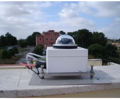
The automatic sky imaging system used for this experiment is the SRF-01 Cloud Cam[9]by EKO, supplied with a control software and a cloud recognition software. When sky images are captured, cloud fraction is calculated by the software with flexibility in the definition of the area of interest by horizon masking and zenith masking. The SRF-01 Cloud Cam, and related software, were installed at Re.S.M.A., on the roof of the local weather station and then connected to a computer through a standard Ethernet interface. A picture of the Cloud Cam is showed in figure 1. The main device consists of a Canon Power Shot A60 digital camera in a weatherproof housing, with a maximum resolution of 1600 x 1200 pixels. Additional optics extend the field of view to 180°, providing the possibility to make color pictures of the whole sky. The system also includes weatherproof connectors, power supply and a dry air pump to avoid condensation effect inside the glass dome. The system supports a data volume of about 60MB/day (1 picture every 10min).
Fig. 1. Cloud Camera installed on the roof of the Vigna di Valle weather station.
The main function of the camera control software is to connect and control the camera from the host PC, where the current image and cloud camera status is showed. A dialog box allows to set shooting options such as aperture and shutter, to define luminosity of the image, day periods of images acquisition, time interval between shots, the file name suffix, to assign a clear name to the parameter set for images identification.
The system allows to make pictures with standard exposure time and under exposure time. Pictures (jpeg-format) are saved in a user-defined folder and processed using the cloud recognition software called “Find Clouds”. The software combines the two images to recognize the full sun light and to eliminate its contribution without the need of a shading device.
The Cloud Cam measures the total cloud amount as the “the fraction of the celestial dome covered by all clouds visible” [7] and it is then estimated by the software returning a value between 0 (sky clear) and 1 (total coverage). The Cloud Cam evaluation is also affected by errors, coming mainly from diffusive effect on the dome, solar aureole or thin cirrus undetected. For these reasons, in this paper the two kind of observations, manned and automatic, are considered on the same plane (none is chosen as reference).
The PC clock were set on U.T.C. and the daily time interval of images acquisition was from 5 a.m. to 9 p.m. The Cloud Camera was set to acquire 2 photos every 10 minutes. The first one is well exposed (aperture = 1/500 and shutter = 8.0 ), the second one is lightly under exposed (aperture = 1/1000 and shutter = 8.0 ). Each of the photos has a proper suffix name in order to correctly
process the images for sun identification. In this experiment the zenith angle was set to 45° in order to match the cloud cover observing specifications of the local manned weather station. Besides, this angle excludes, from the camera view, other meteorological instruments installed on the same horizontal plane.
Finally, for further optimization of images acquisition, a daily cleaning of the glass dome was performed by personnel of the local weather station. This allowed to reduce diffusive effects of the dome, due to dust or water drops on the glass.
METHODOLOGY
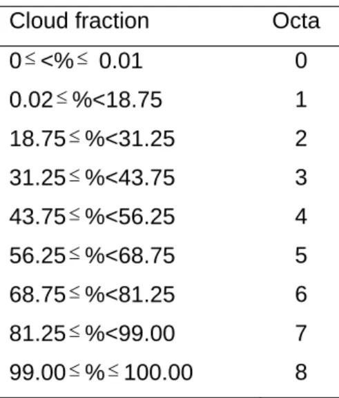
As the Human Observer and the Cloud Cam use two different measurement units for the cloud amount evaluation, the percentage of cloud amount from the Cloud Cam was converted into octa using the conversion criteria showed in table 1 [5]. Moreover, only the sky pictures acquired 10 minutes before the hour were used for the cloud fraction evaluation and comparison.
Table 1. Conversion table from percentage of cloud fraction to octa. Cloud fraction Octa
0<% 0.01 0 0.02%<18.75 1 18.75%<31.25 2 31.25%<43.75 3 43.75%<56.25 4 56.25%<68.75 5 68.75%<81.25 6 81.25%<99.00 7 99.00%100.00 8
For the measurements comparison the statistical approach of the contingency table was used. A contingency table or matrix is essentially a display format used to analyze and record the relationship between two or more categorical variables. It is the categorical equivalent of the scatter plot used to analyze the relationship between two continuous variables. In this case the variables to be compared were the cloud amount in octa measured by the Human Observer and the cloud cam cloud fraction converted into octa. This method gave indications at a glance about overestimation and underestimation of one observation with respect to the other and could evidence the percentage of cases where the comparison yielded differences within 2 octa, 1 octa or the coincidence (diagonal of the matrix). The contingency table approach was used firstly in the preliminary optimization phase to recognize which of the camera settings could give the best contingency with the human observer. In this case the main differences between the two methods of observation were attributed mainly to the incorrect recognition of the solar disc and aureole. As shown in fig. 3 and fig. 4, a marked under-exposition for the second photo needed to recognize the sun, makes the sun red marker very little and sun aureole contributes on the cloud fraction computation. A lesser under-exposition, instead, makes the sun red marker bigger and comparable with the sun aureole. Once the optimum settings were chosen, the same statistical approach was used to compare the two measurements methods for the period of interest.
Fig. 3. Example of photos of normal exposed sky, marked underexposed sky and final evaluation with equalized range and red marker on sun position.
Fig. 4. Example of photos of normal exposed sky, lesser underexposed sky and final evaluation with equalized range and red marker on sun position. In this case some reflectivity effects on the dome are present.
Once Normal Exposed/Underexposed levels was chosen to 2.5 and 2.4 respectively, in order to better evaluate transparent clouds, two shooting options for the under-exposed photos were selected and analyzed by contingency tables (fig. 5 and fig. 6):
- Shooting option Nr.1 (fig.5) with well exposed image with aperture = 1/500 and shutter = 8.0 and under-exposed image with aperture = 1/2000 and shutter = 8.0.
- Shooting option Nr. 2 (fig. 6) with well exposed image with aperture = 1/500 and shutter = 8.0 and under-exposed image with aperture = 1/1000 and shutter = 8.0.
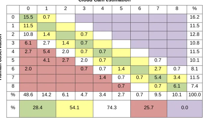
All data in the tables are in percentages. The color coding expresses the degree of agreement between the outputs of the two procedures for cloud cover estimation. If the cell is green, both procedures yield the same cloudiness in octa. If it is yellow there is 1 octa difference and if is white there are 2 octa difference. For purple and violet cells the difference between procedures is larger than 2 octa.
The shooting option Nr. 2 is clearly better than the previous one, reaching the percentage of 85.8% of agreement between human observation and automatic estimation within 2 octa difference and for this reason it was chosen as standard setting for the experiment.
Cloud Cam estimation 0 1 2 3 4 5 6 7 8 % Human observation 0 15.5 0.7 16.2 1 11.5 11.5 2 10.8 1.4 0.7 12.8 3 6.1 2.7 1.4 0.7 10.8 4 2.7 5.4 2.0 0.7 0.7 11.5 5 4.1 2.7 2.0 0.7 0.7 10.1 6 2.0 0.7 0.7 1.4 2.7 0.7 8.1 7 1.4 0.7 0.7 5.4 3.4 11.5 8 0.7 0.7 6.1 7.4 % 48.6 14.2 6.1 4.7 3.4 2.7 0.7 9.5 10.1 100.0 % 28.4 54.1 74.3 25.7 0.0
Fig. 5. Contingency table for human observation and automatic estimation for day time cloud coverage, from May 23rd to June 3rd, related to the shooting option Nr.1.
Cloud Cam estimation
0 1 2 3 4 5 6 7 8 % Human observation 0 13.5 2.7 16.2 1 10.1 1.4 11.5 2 7.4 4.7 0.7 12.8 3 2.7 6.1 1.4 0.7 10.8 4 5.4 4.1 1.4 0.7 11.5 5 1.4 4.1 2.0 1.4 0.7 0.7 10.1 6 0.7 0.7 0.7 2.7 2.0 1.4 8.1 7 0.7 8.1 2.7 11.5 8 0.7 0.7 6.1 7.4 % 33.8 21.6 8.8 4.1 3.4 2.7 4.1 11.5 10.1 100.0 % 35.1 62.2 85.8 14.2 0.0
Fig. 6. Contingency table for human observation and automatic estimation for day time cloud coverage, from May 23rd to June 3rd, related to the shooting option Nr.2.
RESULTS
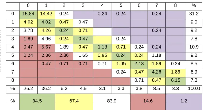
The optimized shooting option was used to compare the Cloud Cam results against the Human Observer for one month of operation (from the 23rd of May 2012 to the 24th of June 2012). The time period considered allowed to test various kinds of cloud coverage so that it could be considered representative of several atmospheric conditions. Only data from 5.00 a.m. UTC till 6.00 p.m. UTC (daytime) were considered for the comparison and the images acquired 10 minutes before the hour were used for a total of 423 data points used for this comparison. Results are summarized in the contingency table showed in fig.7. Calculations were made with full numbers while rounded values were inserted in the table.
Cloud Cam estimation
0 1 2 3 4 5 6 7 8 % Human observation 0 15.84 14.42 0.24 0.24 0.24 0.24 31.2 1 4.02 4.02 0.47 0.47 9.0 2 3.78 4.26 0.24 0.71 0.24 9.2 3 1.89 4.96 0.24 0.47 0.24 7.8 4 0.47 5.67 1.89 0.47 1.18 0.71 0.24 0.24 10.9 5 0.24 2.36 2.36 1.65 0.95 0.24 0.24 1.18 9.2 6 0.47 0.71 0.71 0.71 1.65 2.13 1.89 0.24 8.5 7 0.24 0.47 4.26 1.89 6.9 8 0.71 0.47 6.15 7.3 % 26.2 36.2 6.2 4.5 3.1 3.3 3.8 8.5 8.3 100.0 % 34.5 67.4 83.9 14.6 1.2
Fig. 7. Contingency table built for the testing period.
The octa in the horizontal direction represent the data from the Cloud Cam while the ones in the vertical direction are those from the Human Observer. The color coding expresses the degree of agreement between the outputs of the two procedures. The percentage of cases in the green boxes represents the occurrence of the same octa for the two measurements, the ones in the yellow boxes differs of 1 octa from each other while the white boxes indicate a difference of 2 octa between the two observations. The column and rows denoted by “%” give the percentage of observations for each octa for Cloud Cam and Human Observer, respectively. The row at the bottom of the table summarizes the grade of agreement. So, for 34.5% of the cases the two procedures exhibit the same octa value; for 67.4% of the cases there is a maximum of 1 octa difference between the two and finally in the 83.9% of the cases the two results are within 2 octa. For purple and violet cells difference is larger than 2 octa. In particular for the 14.6% of the cases the Cloud Cam underestimate the cloudiness value with respect to the Human Observer while for the 1.2% of the cases an over estimation of the Cloud Cam was observed. Overestimation and underestimation values were carefully checked to try to understand the reason of these high discrepancies. In particular, the overestimation, much less frequent than the underestimation, was correlated to a single event occurred on the 20th of June where a particular pearlescent sky was observed. Comparison with other kind of measurements (irradiance and spectral irradiance) could be used to better understand this particular phenomenon. The percentage of underestimation values, indeed, was easily correlated with the presence of thin cirrus clouds that are not easily detected by the Cam and with the human observation of a wider field of view than the camera (clouds at the horizon). Also low illumination can be responsible of underestimation.
The obtained agreement is also enforced by the high correlation coefficient (0.88) of the two dataset.
CONCLUSIONS AND DISCUSSION
The project CL.E.A.R developed with the aim to investigate the possibility of automatic cloud recognition for application to meteorological and climate research as well as to renewable energies research has given encouraging results. In particular, the comparison of cloud fraction automatically calculated from sky pictures with human observer estimations of cloud coverage, shows that more than 34% of observations completely match, while for about 84% of them the difference is within 2 octa.
Besides, a part of discrepancy between the two methods of observation is due to the wider field of view of the human observer, that have to report significant cumulus even if they are lower than the 45° zenith angle, configured as field of view in the Cloud Camera.
However, the acquisition and the data elaboration phases underlined some criticalness of the automatic recognition method:
- reflectivity effects on the dome, as for example in fig.4, that can misled the sun identification;
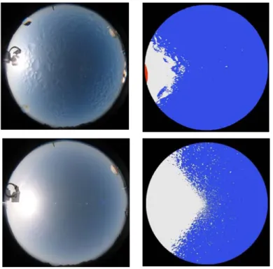
- scattering effects in the case of wet dome (fig. 9 – first row) or in case of particular atmospheric conditions (fig. 9 – second row) as the presence of thin and transparent cirrus. - the automatic sky imaging system needs of a proper solar filter in order to eliminate the sun
aureole errors.
To quantify the above mentioned issues and increase the statistical population, more images are surely needed, by sky photos acquisition follow-on.
Fig. 9. Example of critical images for cloud recognition: (first row) scattering effects for wet dome; (second row) atmospheric scattering effects.
ACKNOWLEDGEMENTS
The authors wish to thank MISURE Company for kindly providing the EKO Cloud Cam used in this experiment and TECNOEL, in particular Tommaso Vitti, for the installation and assistance.
REFERENCES
[1] Martinez-Chico M., F.J. Batles and J.L. Bosch, 2011. “Cloud classification in a Mediterranean location using radiation data and sky images”, Energy 36, pp. 4055-4062
[2] Tomson T., 2010. “Fast dynamic processes of solar radiation”, Solar Energy 84, pp. 318–323. [3] Luo L., D. Hamilton, B. Han, 2010. “Estimation of total cloud cover from solar radiation observations at Lake Rotorua, New Zealand”, Solar Energy 84, pp. 501–506.
[4] Wauben, W. M. F., 2002. “Automation of visual observations at KNMI: (ii) Comparison of automated cloud reports with routine visual observations”, paper presented at Annual Meeting, Am. Meteorol. Soc. (AMS), Orlando, Fla.
[5] Boers, R., M. J. de Haij, W. M. F. Wauben, H. Klein Baltink, L. H. van Ulft,M. Savenije, and C. N. Long, 2010. “Optimized fractional cloudiness determination from five ground‐based remote sensing techniques. Journal of Geoph. Res., 115, pp.1-16.
[6] DIRETTIVA MET RT 1 - REGOLAMENTO TECNICO N.1, 2001. Norme tecnico - operative per l’assistenza meteorologica alla navigazione aerea. Aeronautica Militare - Ufficio Generale per la Meteorologia.
[7] CIMO_Guide-7th_Edition-2008.
[8] Rafanelli, et al. 2005. “Automatic cloud-coverage evaluation by a ground-based Total-Sky Camera, INSTRUMENTS AND OBSERVING METHODS - REPORT No. 82- WMO/TD-No. 1265- (TECO-2005) Bucharest, Romania, 4-7 May 2005.
[9] SRF-01 Cloud Cam - Introduction Manual Version 1, 2012. EKO INSTRUMENTS CO., LTD.