Ion current and exhaust gas composition measurements for combustion monitoring

(1)

DEPARTMENT

OF

INFORMATION

ENGINEERING

AND

MATHEMATICS

Doctor of Philosophy program in

INFORMATION ENGINEERING AND SCIENCE

Ion current and exhaust gas composition

measurements for combustion monitoring

Supervisor:

Professor Valerio Vignoli

Candidate: Lorenzo Parri

Cycle XXXIII

a.a. 2019/2020

(2)

(3)

1

1. Introduction

The efficiency of combustion processes is assuming nowadays a huge importance, since the energy production, many industrial processes, as well as building heating systems are still mainly based on the combustion of hydrocarbons. The performance of the combustion process depends on many factors and it is a crucial point for the reliability and the efficiency of a plant or a thermal machine that exploits combustion as a primary source of energy. Moreover, the constant increasing of carbon dioxide concentration in atmosphere makes more and more important reducing the emission of this gas as well as the other pollutant/toxic chemical compounds that are produced during combustion. An optimized combustion process allows reducing dramatically the production of chemical compounds like carbon monoxide or nitrogen oxides, and also to releasing in the atmosphere the minimum amount of carbon dioxide per unit of energy produced. There are many studies related to the optimization of the internal combustion of the engines (see e. g. [1] and the references therein), especially for automotive applications, whereas the literature is less exhaustive for burner combustion optimization.

The focus of this work is the study and the development of measurement systems allowing to get information about the combustion characteristics in gas turbines, with the aim of providing tools for monitoring/controlling the combustion parameters and keeping the combustion efficiency as high as possible over time. This activity has been developed in collaboration with Beker Huges (Nuovo Pignone Tecnologie - Florence), one of the world leaders in the design and development of gas turbines.

Two different sources of information on the state of the combustion process have been considered in this thesis, namely the density of ions produced by the flame in the combustion chamber and the composition of the exhaust gases.

The measurement of the ionic density due to the flame has been used since several years, particularly in the automotive sector, to obtain information about the combustion process [2] [3]: from the postprocessing of the signal obtained using ionization sensors (or ionic current sensors), it is

(7)

5

possible to determine, for example, the onset of the combustion, the air–fuel ratio (and therefore the pollutant concentration at the exhaust), as well as to get information about the flame stability and the occurrence of periodic pressure variations in the combustion chamber [4]. On this basis, even if the relationship between combustion parameters and flame induced ion density is highly dependent on the type of fuel, there is room to exploit the information of the ion sensors also with gas turbines, to optimize the operation of the combustor (e.g. reducing instability) and to monitor the polluting emissions.

Ion or ionization sensors, which are usually used to measure the ion density in a burning gas, are essentially conductive electrodes capable of generating signals for either the charge transferred to/from the ionized gas and/or the charge induced on the electrodes themselves. The challenging issue concerns the choice of the materials for the sensor (electrodes and electrical insulators) which, being placed in the combustion chamber, must operate in extreme conditions, i.e., for example, in presence of very high temperatures. On the other hand, the conditioning front-end electronics for this kind of sensors is not critical.

As far as the measurement of the concentration of toxic/pollutant compounds in exhaust gases is concerned, the most relevant compounds to be considered are carbon monoxide (CO) and nitrogen oxides (NOx). Monitoring CO and NOx in the exhaust gases is important not only from the point of view of environmental pollution, but also because their concentrations are useful and reliable indicators about the combustion efficiency. The drawback is that, due to the measurement procedure, they cannot be used for a timely feedback control of the combustion process, the reason is that the exhaust gases must be sampled from the chimney and pumped to the measurement instrument (gas analyser), and this procedure introduces a significant delay between the instant in which the gases are produced by the combustion and the time at which they are analysed.

From the standpoint of the measurement instruments, exhaust gas analysers with different accuracies and costs (which are usually relevant) are available on the market. These devices can be portable or fixed and can exploit different measurement principles. Besides cost, an issue of these devices is that accurate gas sensors need frequent calibration exploiting reference gas tanks, which can be a problem in specific industrial plants such as power generation or oil and gas plants. The possibility to use a more flexible gas analyser, with a better trade-off among cost, measurement accuracy, the calibration intervals and robustness, is a deeply felt need in the oil & gas sector,

(8)

6

considering also that these instruments are required to operate in environments that can be severely harsh, especially in terms of temperature and humidity.

In this thesis, the development and testing, in laboratory and in actual test rigs, of two measurement instruments, one for ion current measurements and one for exhaust gas composition measurement is discussed. For the first instrument, a theoretical model of the ion sensor used was also developed, which significantly helped in interpreting the experimental data.

In detail, a brief discussion about the relationships linking the different parameters used in gas turbines combustion control, as well as about ion generation and measurement in combustion processes is presented in section 2. In the same section, a tool exploited to model the burner used for the experiments, which allowed to have a preliminary description of the relationships among the quantities of interest for the ion current measurements, is also presented. The developed model for the ion measurement probe is presented in section 3. In section 4 and 5, the experimental setup and the obtained measurements are discussed. In section 6 an overview of the possible exhaust gas measurement techniques is reported, whereas in section 7 the architecture of the designed instrument for exhaust gas analysis is presented. Finally, before the conclusions, in section 8 the tests on the field of the designed gas analyser are presented and discussed.

(9)

7 1.1 Contributions

A) T. Addabbo, A. Fort, M. Mugnaini, L. Parri, V. Vignoli, M. Allegorico, M. Ruggiero and S.

Cioncolini, “Ion Sensor-Based Measurement Systems:Application to Combustion Monitoring in Gas Turbines,” IEEE Transactions on Instrumentation and Measurement, vol. 69, no. 4, 2020.

B) Tommaso Addabbo, Ada Fort, Marco Mugnaini, Lorenzo Parri, Stefano Parrino, Alessandro

Pozzebon, Valerio Vignoli, “A low power IoT architecture for the monitoring of chemical emissions.” Published in: Acta Imeko 8.2 (2019): 53-61.

C) A. Pozzebon, A. Fort, E. Landi, M. Mugnaini, L. Parri, V. Vignoli. “A LoRaWAN Carbon

Monoxide Measurement System with Low-Power Sensor-Triggering for the Monitoring of Domestic and Industrial Boilers., IEEE Transactions on Instrumentation and Measurement, Ref.: Ms. No. TIM-20-01622R2

D) Addabbo, T., Bardi, F., Cioncolini, S., Fort, A., Mugnaini, M., Parri, L., Vignoli, V.

“Multi-sensors exhaust gas emission monitoring system for industrial applications.”, (2019) Lecture Notes in Electrical Engineering, 512, pp. 49-56.

E) T. Addabbo, A. Fort, M. Mugnaini, L. Parri, V. Vignoli, M. Allegorico, M. Ruggero, S.

Cioncolini. “Ion sensors: application to combustion monitoring in gas turbines”, 2019 IEEE Sensors Applications Symposium (SAS), Sophia Antipolis, France, 2019, pp. 1-6. doi:

10.1109/SAS.2019.8706114

F) Addabbo, T., Fort, A., Mugniani, M., Parri, L., Vignoli, V. “An unconventional type of

measurement with chemoresistive gas sensors exploiting a versatile measurement system”, (2017) Proceedings - 2017 1st New Generation of CAS, NGCAS 2017, art. no. 8052282, pp. 113-116.

G) Addabbo, T., Fort, A., Mugnaini, M., Parri, L., Parrino, S., Pozzebon, A., Vignoli, V., “An

IoT Framework for the Pervasive Monitoring of Chemical Emissions in Industrial Plants.”, (2018) 2018 Workshop on Metrology for Industry 4.0 and IoT, MetroInd 4.0 and IoT 2018 - Proceedings, art. no. 8428325, pp. 269-273.

(10)

8

H) T. Addabbo, A. Fort, M. Mugnaini, L. Parri, A. Pozzebon, V.Vignoli., “Smart Sensing in

Mobility: a LoRaWAN Architecture for Pervasive Environmental Monitoring.”, 2019 IEEE 5th International forum on Research and Technology for Society and Industry (RTSI), Florence, Italy, 2019, pp. 421-426, doi: 10.1109/RTSI.2019.8895563.

I) T. Addabbo, A. Fort, M. Intravaia, M. Mugnaini, L. Parri, A. Pozzebon, V. Vignoli.,

“Pervasive environmental monitoring by means of self-powered Particulate Matter LoRaWAN sensor Nodes.”, Imeko tc4 2020, Palermo.

(11)

9

2. Combustion Control: the possible role of ion

density measurements

Combustion control of gas turbines is a complex topic that is not dealt in this thesis. Just a few considerations are reported to introduce the framework in which the research activity was developed.

Figure 2.1 . A gas turbine structure

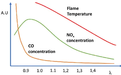
The combustion control strategy for a gas turbine is set up during the machine tuning procedure. Among all the quantities monitored, two are more directly linked to the combustion: the exhaust gases composition and the pressure pulsations in combustion chamber. Pulsation phenomena consist of rapid changes of pressure in combustion chamber caused by a not correct combustion of the fuel. These events must be avoided because they may be dangerous for the machine integrity. The flame temperature is directly proportional to the output power and it is not directly measured, but is calculated knowing the fuel chemical composition, and the air flow.

Usually, an increase of flame temperature causes an increase of pressure pulsations and NOx concentration in the exhaust gases, and a decrease of flame temperature causes a decrease of NOx concentration as shown in Figure 2.2 [5]. The flame temperature depends on several factors but it is mainly determined by the lambda factor (𝜆), i.e. the ratio between the mass of air and the mass of fuel used to supply the burners divided by the stoichiometric air to fuel ratio. The ideal lambda factor (𝜆 = 1) can be calculated knowing the chemical composition of the fuel: a lambda factor <

(12)

10

1 indicates that more fuel than required is supplied: in this condition the flame will be more stable but with a larger temperature, so the production of NOx compounds will increase. If the lambda factor is greater than one, more air than required is supplied, and the flame temperature and the production of NOx will decrease. The formation of CO is usually proportional to the presence of not completely combusted elements. In case of very low lambda factors the concentration of CO can dramatically increase whereas for larger lambda values the CO concentration gets lower because almost all the fuel is easily burned. Unfortunately, the CO concentration is very hard to be predicted, the formation causes of this gas during combustion are complex and, in some cases, not completely known. This is the main reason for which it is still very important to measure CO concentration. Operating at high lambda values is a good choice in terms of efficiency and emission of toxic compounds, but the flame becomes less stable and the control of the combustion becomes harder.

Figure 2.2 – Qualitative plot of flame temperature, CO and NOx emission concentrations as a function of lambda factor. (A.U.: arbitrary units)

From this brief introduction it can be easily understood how much an efficient control of the combustion is important for a gas turbine burner. Nowadays, the demand on the market of low emission machines is increasing, and the combustion control is becoming an even more critical aspect.

(13)

11

The ion current measurement is a promising technique to easily control the conditions of the combustion, and a cheap versatile and portable instrument to monitor the chemical composition of exhaust gases can be of great use and application in the oil and gas sector. An accurate condition monitoring of burners makes easier to program the preventive maintenance, and to keep the combustion process in optimal conditions over the time, reducing maintenance costs and emission of toxic compounds, while increasing the efficiency.

2.1 Ion Current Measurement: State of the art

Measurement of the ionic density in the burning gases have been used for several years, particularly, in the automotive sector, to obtain information about the combustion process [2], [3]. Although the relationship between combustion parameters and ionic density in the flame is strongly dependent on the type of fuel, it is documented in the literature that, from the postprocessing of the signal obtained using ionization sensors (or ionic current sensors), it is possible to determine, for example, the occurrence of pressure dynamics, the onset of combustion, the air–fuel ratio, and the flame stability [4]. Therefore, ion sensor information could be used to optimize the combustor operations (e.g., reducing the instabilities) and to monitor pollutants emission, which is of particular interest today.

Ion sensing is based on immersing one or two metal electrodes in the flame where exothermic chemical reactions release a large amount of ions (chemo-ionization) and sensing their concentration, either biasing the electrodes and measuring the current due to the drift of ions forced by the external applied electrical field, or by using unbiased electrodes and by measuring the charge induced in the electrodes by the ions/electrons freely moving in front of the electrodes themselves [6]. The signal thus obtained depends on the ion concentration in the flame and allows for monitoring many combustion process characteristics, among which pressure pulsations that affect the ion concentration locally, besides simply indicating the presence of the flame.

In general, many different monitoring applications through ion sensors have been proposed for combustors or combustion engines, mainly for endothermic alternative engines, more rarely for rotative ones [7] [8] [9] [10] [11] [12] [13] [14] [15] [16] [17]. The simplest successful application is

(14)

12

flame detection, but recently many studies propose systems with enhanced monitoring capability from crank angle in diesel engines to burning gas characteristics in gas turbines. In these studies, some efforts were devoted to understanding and modeling the sensor behavior, but actually a thorough model still lacks. On the other hand, the same sensor structure and sensing strategy is used, studied and modelled for plasma studies in different application fields (plasma based material processing and aerospace application) and it is called Langmuir probe.

2.2 Ion Current theoretical background

The combustion of hydrocarbons is accompanied by the generation of a large quantity of ions by a process called “chemoionization”. The main reactions that allow for the formation of ions are listed in Table 1 [18] [19] [20]. In the table the parameters A, υ and Ea define the reaction rate

constant k according to the Arrhenius equation (1), R is the universal perfect gas constant and T

the absolute temperature, supposing to have second order reactions:

𝑘 = 𝐴 𝑇𝜐 𝑒 −𝐸𝑎𝑅𝑇 (1) Step Reaction A [𝑐𝑚3 𝑚𝑜𝑙 𝑠 𝑇 −𝜐_] _𝝊 _𝐄 𝐚[ 𝑘𝐽 𝑚𝑜𝑙] 1 𝐶𝐻 + 𝑂 → 𝐶𝐻𝑂+_{+ 𝑒}− _{2.31 ∙ 10}11 _0.00 _7.12 2 𝐶𝐻𝑂+_{+ 𝐻} 2𝑂 → 𝐻3𝑂++ 𝐶𝑂 1.00 ∙ 1016 −0.09 0.00 3 𝐶𝐻𝑂+_{+ 𝐶𝐻} 2 → 𝐶𝐻3++ 𝐶𝑂 5.62 ∙ 1014 0.00 0.00 4 𝐶2𝐻3𝑂++ 𝑂 → 𝐶𝐻𝑂++ 𝐶𝐻2𝑂 2.00 ∙ 1014 0.00 0.00 5 𝐶𝐻3+ + 𝐻2𝑂 → 𝐶2𝐻3𝑂++ 𝐶𝐻2 7.24 ∙ 1014 0.00 0.00 6 𝐶2𝐻3𝑂++ 𝑒− → 𝐶𝐻2𝐶𝑂 + 𝐻 2.29 ∙ 1018 −0.50 0.00 7 𝐻3𝑂++ 𝑒− → 𝐻2𝑂 + 𝐻 2.29 ∙ 1018 −0.50 0.00 8 𝐻3𝑂++ 𝑒− → 𝑂𝐻 + 𝐻 + 𝐻 7.95 ∙ 1018 −1.37 0.00 9 𝐶𝐻𝑂+_{+ 𝑒}−_{→ 𝐶𝑂 + 𝐻} _{7.40 ∙ 10}18 _−0.68 _0.00

(15)

13

A general reaction scheme for the complete combustion of hydrocarbons is the following:

𝐶_𝑥𝐻_𝑦 + (𝑥 + 𝑦

4) 𝑂2 → 𝑥 𝐶𝑂2 + 𝑦

2𝐻2𝑂 (2)

The reaction can also be also incomplete, in this case ions species can be formed together with the formation of carbon monoxide:

𝐶𝑥𝐻𝑦 + ( 𝑥 2+ 𝑦 4) 𝑂2→ 𝑥 𝐶𝑂 + 𝑦 2(𝐻3𝑂 +_{+ 𝑒}−₎ (3)

This situation can be due to a deficit of oxygen or can be an intermediate step of the complete reaction as shown in reaction (4):

𝑥 𝐶𝑂 + ( 𝑥

2 ) 𝑂2 → 𝑥 𝐶𝑂2 (4)

Among all the possible reactions, the main source of ions comes from the first reaction shown in Table 1.

𝐶𝐻 + 𝑂 𝑘1→ 𝐶𝐻𝑂+_{+ 𝑒}− ₍₅₎

The CHO+_{species is not the dominant one in the flame because it rapidly reacts with water, that}

is widely present in exhaust gases, generating H3O+ ions as shown in the second reaction of Table

1.

𝐶𝐻𝑂+_{+ 𝐻} 2𝑂

𝑘2

→ 𝐶𝑂 + 𝐻₃𝑂+ ₍₆₎

The reaction rate constant of step 2 in Table 1 (k2) is much faster than the reaction constant of the

step 1 (k1), therefore the dominant species becomes H3O+. From Table 1 there are many other

(16)

14

predominant species is H3O+. There is a limitation to ion density due to the recombination of H3O+

with free electrons [21] as shown in equation (7):

2𝐻3𝑂+ + 2𝑒− 𝑘4

→ 2𝐻2𝑂 + 𝐻2 (7)

This reaction is very fast with respect to the ion formation but the probability of collision of electrons with H3O+ is very small [21]. The free electron density is also reduced due to the presence

of electronegative species such as O- _{or OH}-_.

The reactions in a flame are not instantaneous and they take place in different areas. The probability of presence of different chemical species in different areas of the flame can be significantly different.

Considering the reactions (5) and (6), it is possible to write the concentration of ions [CHO+_]1_at

the equilibrium as a function of the reaction rates kx and:

[𝐶𝐻𝑂+] = 𝑘1[𝐶𝐻][𝑂] 𝑘2[𝐻2𝑂] ₍₈₎ Where: 𝑘1 = (2.31 ∗ 1011) 𝑒 −7.12 𝑅𝑇 𝑐𝑚 3 𝑚𝑜𝑙 𝑠 𝑘₂ = ( 1016_{) 𝑇}−0.09 𝑐𝑚 3 𝑚𝑜𝑙 𝑠

As described before, CHO+ _{ions lifetime is relatively short so, by using equation (6) and (7), it is}

possible to write the concentration of [H3O+] at the equilibrium as:

(17)

15

[𝐻₃𝑂+_{] =}𝑘2[𝐶𝐻𝑂 +_][𝐻 2𝑂] 𝑘₄[𝑒−_] (9) Where: 𝑘₄ = (2.29 ∗ 1018_)𝑇−0.5 𝑐𝑚 3 𝑚𝑜𝑙 𝑠

If we consider a neutrality condition, the concentration of electrons and [H3O+] can be considered

the same. Using this consideration and combining equations (8) and (9) it is possible to obtain:

[𝐻₃𝑂+_{] = √}𝑘1

𝑘₄ [𝐶𝐻][𝑂] (10)

In a combustion process it is important to maintain the control of the Air-Fuel equivalence ratio that is has already seen is defined as the ratio between the air to fuel ratio of the combustible mixture and the stoichiometric air to fuel ratio [21].

𝜆 = 𝐴𝐹𝑅 𝐴𝐹𝑅_{𝑆𝑡𝑒𝑐ℎ} ∝ [𝑂] [𝐶𝐻] 𝐴𝐹𝑅_{𝑆𝑡𝑒𝑐ℎ} (11)

Comparing equations (10) and (11) it is evident the correlation between [H₃O+] and λ [21] [22]; with a dependence witch is qualitatively shown in Figure 2.3.

(18)

16

Figure 2.3 - Ion Concentration expected behaviour with lambda. (A.U.: arbitrary units). In general, as lambda increases, [CH] decreases whereas more oxygen then required for the combustion is present, so [H3O+] decreases.

For low values of lambda, the oxygen is not sufficient for a complete combustion, causing a decreasing of [H3O+].

In the last equations we considered a dependence on monoatomic oxygen (O). The monoatomic oxygen is not present at environmental conditions, but this is not true inside the flame. As shown in Figure 2.4 at around 2000 Kelvin the diatomic oxygen can dissociate making possible the presence of monoatomic oxygen.

(19)

17 2.3 Ion Channel

To measure the ion density, it is necessary to transform the presence of charge in the flame in an electrical signal. The classical solution is to apply an electric field across two electrodes and to measure the current flowing between them. This current is due to the ionic channel, between the electrodes, originated by the flame. As a first approximation the ion density is higher in high temperature regions [24].

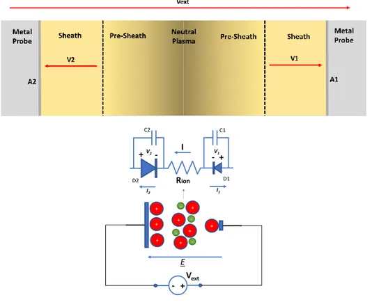
The current is due both: 1) to charged species moving between the electrodes and 2) to the charge transferred from the gas to the electrodes. If a parallel planar electrodes structure is adopted, as in Figure 2.5, it is possible to give a simple description of the measured current assuming that no chemical reactions occur at the electrode interfaces.

Figure 2.5 – Electrodes Geometry

In Figure 2.5 the planar plates are parallel to the xz-plane, we consider an ionized gas flow containing only H3O+ ions moving along the x-axis. Under these assumptions, the following

equations can be considered [19] :

𝜕𝑝_𝑖 𝜕𝑡 + 𝜕𝛤_𝑖,𝑥 𝜕𝑥 + 𝜕𝛤_𝑖,𝑦 𝜕𝑥 = −𝛽𝑝𝑖𝑛 + 𝑘𝑐ℎ𝑒𝑚 (12)

(20)

18

𝜕𝑛 𝜕𝑡 + 𝜕𝛤_𝑒,𝑥 𝜕𝑥 + 𝜕𝛤𝑒,𝑦 𝜕𝑥 = −𝛽𝑝𝑖𝑛 + 𝑘𝑐ℎ𝑒𝑚 (13) 𝜕2_𝜙 𝜕𝑥2 + 𝜕2_𝜙 𝜕𝑦2 = − 𝑞 𝜀 ( 𝑝𝑖 − 𝑛 ) (14)

Where: pi is the cations volume density, n is the electrons volume density, β is the electron-cations

recombination factor, Kchem is the generation rate due to Chemo-Ionization, 𝜞_𝒎,𝒌 is the flow along k of the species m, 𝝓 is the external applied potential, ε is the medium dielectric constant, q is the

electron charge.

Equations (12) and (13) represent the charge flow balance between the electrodes considering having moving ions. The equation (14) considers the application of an external electric potential 𝜙. For Kchem, the generation rate of ions, we consider H3O+ ions according to the previous discussion,

whereas β, the rate of recombination of cations with electrons, is the rate constant k4 in reaction (7). The variation with time of ions and electrons is the rate of generation Kchem minus the

recombination rate and the charge species flow. The charge species flow is a composition of different effects. One is the mechanical transportation due to exhaust gas flow. In addition, there is a drift component due to the external electric field, and a diffusion component due to different ion concentrations, as described by the following equations:

𝛤𝑖,𝑥 = −𝐷𝑖 𝜕𝑝_𝑖 𝜕𝑥 + 𝜇𝑝𝑝𝑖𝐸𝑥+ 𝑝𝑖𝑣𝑓𝑙𝑜𝑤(𝑦) 𝛤_𝑖,𝑦 = − 𝐷_𝑖𝜕𝑝𝑖 𝜕𝑦 + 𝜇𝑝𝑝𝑖𝐸𝑦 (15) 𝛤_𝑒,𝑥 = −𝐷_𝑒𝜕𝑛 𝜕𝑥+ 𝜇𝑒𝑛𝐸𝑥+ 𝑛𝑣𝑓𝑙𝑜𝑤(𝑦) (16)

(21)

19

𝛤𝑒,𝑦 = − 𝐷𝑒 𝜕𝑛

𝜕𝑦 + 𝜇𝑒𝑛𝐸𝑦

Where: 𝝁𝒙 is the mobility of species x, Ek is the electric filed along k, Dx is the diffusion coefficient

of species x, Vflow is the gas flow speed.

In equations (15) and (16), 𝐷𝑥 can be expressed by the Einstein relationship:

𝐷_𝑥 = 𝜇_𝑥 𝐾𝑇

𝑞 (17)

2.3.1 Small External Electric Field Assumption

To simplify the model described by equations (12)(13)(14)(15)(16), some assumption can be considered:

• The chemical reactions are at the equilibrium so:

𝑘_{𝑐ℎ𝑒𝑚} − 𝛽𝑝_𝑖𝑛 = 0 ₍₁₈₎

• The effect of the external electric field in removing electrons or ions from the area of measurement is negligible. This means that the gap between the electrodes can be considered occupied by a neutral plasma (n = pi) and the electric field in reactions (15) and

(16) coincides with the external field applied by the electrodes. This field can be considered constant, having only the y component different from zero (i.e., Ex = 0).

• Vflow, that represents the transportation velocity of charges by the gas flow2, is negligible

with respect to the speed of charges accelerated by the electric field.

2_{The gas flow in a burner has usually a turbulent behaviour: in the proposed model}_V

flow is an

(22)

20

Under these assumptions, the charges flow can be approximated by the following equations: 𝛤_𝑖,𝑥 = 0 𝛤𝑖,𝑦 = 𝜇𝑝𝑝𝑖𝐸𝑦 = 𝐽_𝑖 𝑞 (19) 𝛤_𝑒,𝑥 = 0 𝛤𝑒,𝑦 = 𝜇𝑒𝑛𝐸𝑦 = 𝐽_𝑒 𝑞 (20)

Where Jx is the density of current of species x. The total current, considering a neutral plasma (n = pi) is so given by:

𝐽 = 𝐽_𝑖 + 𝐽_𝑒 = 𝑞( 𝜇_𝑒 + 𝜇_𝑝) 𝑛 𝐸_𝑦 ₍₂₁₎

And we can express the equivalent conductivity of the ionized gas as:

𝜎 = 𝐽 𝐸𝑦

= 𝑞( 𝜇𝑒 + 𝜇𝑝 ) 𝑛 (22)

The density of charges (n=pi) is determined using (18):

𝑛 = 𝑝_𝑖 = √ 𝑘𝑐ℎ𝑒𝑚

𝛽 (23)

The ion channel has, under this assumption, a resistive behaviour since the current is linearly dependent on the applied electric field.

(23)

21

2.3.2 Strong External Electric Field Assumption (Saturation)

Another simplification of the model can be obtained in the limit case in which the external electric field Eyis strong enough that the drift velocity becomes much faster than the electron-ion pair

generation rate. The flows in reactions (15) and (16) is mainly determined in this case by drift component along y. Charges are immediately attracted on the electrodes making impossible the recombination:

𝜕𝑛 𝜕𝑡 =

𝜕𝑝_𝑖

𝜕𝑡 = 𝑘𝑐ℎ𝑒𝑚 (24)

In this situation there is a saturation effect, all the ions pairs generated are attracted by the electrodes and the current becomes independent from the electric field:

𝐽 ∝ 𝑞 𝑘_{𝑐ℎ𝑒𝑚} ₍₂₅₎

Since our target is to measure the ions density it is necessary avoiding to reach the saturation condition, which sets a saturation upper limit to the applied external electric field.

2.4 A Numerical Model for the Burner

The ion distribution density as a function of the lambda parameter can be estimated using a more complete physical model: for this purpose we used Cantera, an open-source suite of tools for problems involving chemical kinetics, thermodynamics, and transport processes [25]. In detail, we exploited the one-dimension model flame to simulate a burner premixed3_{flame: the flames are modelled}

in 1 dimension, by a set of ordinary differential equations (ODE), which is solved in the axial coordinate. The gas flow is physically bidimensional, but a similarity transformation allows to

3_{A premixed flame is a combustion reaction supplied by a homogeneous mixture of fuel and air}

(24)

22

consider a 1D problem. The burner is modelled by a stack of domains. The domains can be gas flows, inlets, outlets, surfaces, or others. Each domain is described by a set of variables and governing equations. The domains are spatially connected by boundary conditions. The solution of the problem is the solution of all the coupled domains. The domain stack used for this work is shown in Figure 2.6.

Figure 2.6 - Bruner Model

The inlet condition is a mixture of air and propane (C3H8). Considering the reaction (2) the

stoichiometric ratio between fuel (propane) and Oxygen is 1:5. Considering that air contains 20.8% of oxygen the AFRStech in (11) is approximately 25. Simulations using different values of AFR,

corresponding to values of  factor from 0.7 to 1.3, were performed. The results in terms of [H3O+]

(25)

23

Figure 2.7 - Ion concentration vs lambda. The concentration is in mole fraction.

(26)

24

Figure 2.9 - Oxygen concentration in mole fraction vs lambda

The model considers only the premixed part of a burner and was useful to verify the expected behaviour of ion concentration with λ. The plots reported in Figure 2.7 and in Figure 2.3, have a similar behaviour. The flame temperature has been considered to check the dependence of ion concentration with local temperature. Higher temperature areas usually correspond to higher ion densities. If lambda increases, the temperature of the flame decreases and therefore also the ion density decreases. This effect was not considered in the theoretical discussion. Obviously, it is impossible to remove this dependence but when lambda is lower than 0.9 the ion density decreases even if the flame temperature does not decrease. This is due to the oxygen concentration, shown in Figure 2.9, that decreases dramatically for lambda ≤ 0.9. The results, even if obtained from a

simplified model, confirm the theoretical analysis according to which the lack of oxygen causes a decrease of ion density.

(27)

25

3 Current Probe Model

In this thesis, based on the Langmuir probe theory, a complete model for the ion sensor is developed and compared with the simpler ion sensor models used in the literature, with reference to the gas turbine field, and considering to exploit as ion-sensor the electrode of the built-in spare spark-plug (even if this approach was already proposed in the literature [26] [27] and the reference therein), a complete modelling of the sensor and of the measuring system specifically aimed at understanding the measurement performance, still lacks). The model refines previous studies by taking into account also the physical effect of the gas/electrode interfaces. Note that chemical or electrochemical effects at this boundary are not accounted for in detail. The model accounts also for the loading effect of the front-end circuit and the overall dynamic behaviour.

The current probe used for ion current measurement in this work is a standard spark plug used to ignite the fuel/air mixture. This is a typical spark plug used for gas turbines or aircraft engines. The electrodes of the probe are shielded by a Pt/30%Rh coating. The spark plug electrodes experience temperatures which are typically between 600 °C and 800 °C. The probe, as shown in Figure 3.1, is asymmetric. One electrode (the smaller one) is in the inner part whereas the other one is in the external part and is usually in contact with the metallic case of the burner.

(28)

26

Figure 3.1 – The spark plug used for ion current measurement. Photograph of the used spark plug (up left). Tip upper view and cross section highlighting the electrode geometry (up-right). The area of the measuring electrode is approximately 4 mm2_{.On the bottom the structure of a typical gas turbine burner that exploit this spark plug is}

shown.

A simplified equivalent circuit for the current probe sensor and the ion channel is shown in Figure 3.2. The resistance (Rion) describes the gas conductance as discussed in (22). The capacitance (C)

represents the double layer capacitances effect, mainly due to the ionic species at the electrode/gas interface. This capacitance can also have a large value.

(29)

27

Unfortunately, the simplified model of Figure 3.2 is effective to describe the measurement results only in specific circumstances, whereas in general a more complex model to describe the probe behaviour is necessary.

3.1 Ions probe physical background [23] [28]

To have an idea of the expected I-V characteristic of ions probes, we need to consider that the electrodes of the probe are close to the flame, where we can consider the presence of a plasma as shown in Figure 3.3. A plasma is an ionized gas that contains free charges (electrons and positive ions or cations) in which the total charge can be considered neutral. In this condition, being the electrodes of the probe made of conductive material, in the plasma, they can be considered a Langmuir probe. The Langmuir probe behaviour is based on the Debye sheath effect. If a metal is put in a plasma, on its external surface a layer of a greater density of positive charges is generated as shown in Figure 3.4. To explain this effect, we need to consider that electrons can be exchanged between metal and plasma, whereas cations cannot enter the metal. For simplicity we suppose that no chemical reactions occur at the metal-plasma interface. This last hypothesis can be considered almost true if a platinum coated probe is used as in our case. Chemical reactions at the interface, like oxidation reactions, can easily take place if a metal like iron is used for the external surface of the probe, making the ion current measurement impossible.

At the onset of the flame, the movement of electrons and cations can be modelled by a diffusion current if no external electric field is applied.

𝐽_𝑒 = −𝑒 𝐷_𝑒𝑑𝜌𝑒(𝑥)

𝑑𝑥 𝐽𝑖 = 𝑒 𝐷𝑖

𝑑𝜌𝑖(𝑥)

𝑑𝑥 (26)

Where De and Di are the diffusion coefficients of electrons and cations, respectively, whereas e(x)

and i(x) are the densities of electrons and cations. The diffusion coefficient of electrons is greater

(30)

28

at the end of a transient phase is balanced by a “sheath” of positive charges around the electrode ( Figure 3.4), which generates a voltage drop at the electrode/plasma interface inhibiting the current (diffusion current + drift current = 0).

Figure 3.3 - Different plasma types as a function of charge density and temperature [23].

(31)

29

To understand the behaviour of a Langmuir probe we need to consider some aspects of the plasma physics. For simplicity we will study a mono dimensional case in which the x coordinate is along the direction orthogonal to the probe surface that is set at x=0 (wall), as shown in Figure 3.5.

Figure 3.5 - Langmuir probe with shown two possible polarizations of the wall with respect to the plasma.

For this study, a collision less Maxwellian plasma is considered in which positive ions or cations (i) and

electrons (n) are present with the same electrical charge e. Let be mi the mass of the positive ions,

me the mass of the electrons, ni the density per unit of length of ions, nethe density per unit of

length of electrons. Vi is the speed of ions while Verepresents the speed of electrons and, finally,

(x) is the electric potential at x. Let also be the electron temperature and the cation temperature Teand

Ti respectively, which are related to the average kinetic energy of electrons and ions. These

temperatures are defined as the variation of the internal energy (U), given a volume containing a given number of particles, with respect to the particles entropy (S).

(32)

30

𝑇 = 𝜕𝑈(𝑆)

𝜕𝑆 (27)

Teand Ti multiplied by the Boltzmann constant (kB) 4, are usually expressed in electron-volt (eV).

From now on we consider the electron/ion temperature in K.

In what follows an analytical expression for the current flowing in the sheath as a function of the voltage between probe and plasma is derived. The total current is the sum of the cations and the electron current contributions. We need to consider both the cases in which the potential of the probe, due to an externally applied voltage, is positive or negative5_{with respect to the plasma}

potential. The sheath edge is defined at x=S but, obviously, this is an approximation because there is not a steep discontinuity between plasma and sheath. We consider, as a first approximation, that the plasma potential is equal to the potential ((S)) in x =S.

3.1.1 Electron current

Let us start with the component of the current given by electrons. We consider first a potential such that 𝛷(𝑆) − 𝛷(0) > 0 (positive potential):

The electrons at x=S are rejected by the potential inside the sheath region. Only electrons with a sufficient kinetic energy can enter in the sheath region. The energy conservation for these particles is: 1 2𝑚𝑒𝑉𝑒 2_{(𝑆) −}1 2𝑚𝑒𝑉𝑒 2_{(0) = 𝑒|Φ(𝑆) − Φ(0)|} (28)

4_{1 eV corresponds to a temperature 11.605 Kelvin.}

5_{Positive or Negative polarization is referred to the Figure 3.5 that is used as a reference. We}

considered a positive polarization the condition in which the plasma potential is greater than the probe potential.

(33)

31

So, the minimum kinetic energy required for the electrons at x=S to enter in the sheath region is: 1

2𝑚𝑒𝑉𝑒

2_{(𝑆) > 𝑒|(Φ(𝑆) − Φ(0)|}

(29)

The minimum speed is therefore given by:

𝑉_𝑒𝑚2(𝑆) = 2|Φ(𝑆) − Φ(0)|

𝑚_𝑒 (30)

The plasma is neutral ( 𝑛𝑖 = 𝑛𝑒 = 𝑛𝑝), but in the sheath region this is not true (𝑛𝑖 ≠ 𝑛𝑒). To maintain the continuity of the electron charge species flow it is necessary to have that:

𝐽_𝑒 = 𝑒 𝑛_𝑒(0)|𝑉𝑒(0)| = 𝑒 𝑛𝑒(𝑆)|𝑉̅̅̅̅̅̅̅| = 𝑒 𝑛𝑒(𝑆) 𝑒(𝑥)|𝑉𝑒(𝑥)| 𝑛_𝑒(𝑆) ≃ 𝑛_𝑝

𝑥 ∈ [0, 𝑆]

(31)

Where Jeis the electron current density, the electron density at the edge of the sheath can be

considered equal to the plasma density.

The electron speed at the sheath edge can be found considering a Maxwellian distribution. The speed probability density function for a mono dimensional (x) Maxwell-Boltzmann distribution is:

𝑓_𝑣𝑒(𝑣𝑒𝑥) = √ 𝑚𝑒 2𝜋𝑘_𝐵𝑇_𝑒 𝑒

− 𝑚𝑒𝑣𝑒𝑥2

2𝑘𝐵𝑇𝑒 ₍₃₂₎

The average speed of electrons at x=S, |𝑉̅̅̅̅̅̅̅̅|, can be found considering the probability density _𝑒+_(𝑆) function in (32) and velocities greater than Vem(S):

(34)

32

So, using the equation (31), the current density when a positive potential is present, 𝐽𝑒+, is given by:

𝐽_𝑒+ = 𝑒 √𝑘𝐵𝑇𝑒

2𝜋𝑚_𝑒 𝑛𝑒(𝑆) 𝑒

− 𝑒 |Φ(𝑆)−Φ(0)|

𝑘𝐵𝑇𝑒 (34)

Let us now suppose to apply an external potential such that Φ(𝑆) − Φ(0) < 0 (negative potential). In this case, electrons are attracted into the sheath. Considering again a Maxwellian distribution for the electrons we can write that the average electron speed is6_:

|𝑉̅̅̅̅̅̅̅̅ | = 𝐸[𝑣_𝑒−_(𝑆) 𝑒𝑥] = ∫ √ 𝑚_𝑒 2𝜋𝑘_𝐵𝑇_𝑒 𝑒 − 𝑚𝑒𝑣𝑒𝑥2 2𝑘𝐵𝑇𝑒 𝑖𝑛𝑓 0 𝑣_𝑥 𝑑𝑣_𝑥 = √𝑘𝐵𝑇𝑒 2𝜋𝑚_𝑒 (35)

The negative potential attracts electrons into the sheath: supposing that electrons move at X=S at 𝑉_𝑒−_(𝑆)

̅̅̅̅̅̅̅̅ , the speed at x=0 due to the potential acceleration of the electrons can be derived from equation (28):

|𝑉̅̅̅̅̅̅̅̅ |_𝑒−₍₀₎ 2₌2𝑒|Φ(𝑆) − Φ(0)|

𝑚_𝑒 + |𝑉̅̅̅̅̅̅̅̅ |𝑒−(𝑆) 2

(36)

6This result does not take into account the effect of the presheath region and the Bohm’s

(35)

33

Supposing constant, as a first approximation (small values of Φ(𝑆) − Φ(0)), the electron’s density in the sheath in case of negative polarization [29], the current density, 𝐽𝑒−, can be expressed as:

_𝐽_𝑒− _{= 𝑒 𝑛} 𝑝|𝑉𝑒−(0)| = 𝑒 𝑛𝑝√ 𝑘_𝐵𝑇_𝑒 2𝜋𝑚_𝑒+ | 2𝑒(Φ(𝑆) − Φ(0)) 𝑚_𝑒 | ₍₃₇₎

3.1.2 Ion current

When a positive potential ( Φ(𝑆) − Φ(0) > 0 ) is considered, the cations at the edge of the sheath are attracted to the wall since the wall is negatively biased with respect to the plasma. We can write the same energy conservation equation as electrons:

1

2𝑚𝑖𝑉𝑖(𝑆) 2₋1

2𝑚𝑖𝑉𝑖(0)

2 _{= −𝑒|Φ(𝑆) − Φ(0)|} ₍₃₈₎

The speed of cations at the sheath interface can be obtained as for electrons exploiting the Boltzmann distribution. The speed probability density function of a monodirectional Maxwell-Boltzmann distribution (x), is for cations:

𝑓𝑣𝑖(𝑣𝑖𝑥) = √ 𝑚_𝑖 2𝜋𝑘𝐵𝑇𝑖 𝑒 − 𝑚𝑖𝑣𝑖𝑥2 2𝑘𝐵𝑇𝑖 ₍₃₉₎

The average speed of cations, analogously to what seen for the electrons, is given by7_:

|𝑉̅̅̅̅̅̅̅̅ | = 𝐸[𝑣_𝑖+_(𝑆) 𝑖𝑥] = ∫ √ 𝑚𝑖 2𝜋𝑘_𝐵𝑇_𝑖 𝑒 − 𝑚𝑖𝑣𝑖𝑥2 2𝑘𝐵𝑇𝑖 𝑖𝑛𝑓 0 𝑣_𝑥 𝑑𝑣_𝑥 = √𝑘𝐵𝑇𝑖 2𝜋𝑚_𝑖 (40)

7This result does not take into account the effect of the presheath region and the Bohm’s

(36)

34

The effect of 𝛷(𝑆) > 𝛷(0) is that the ion’s velocity at the electrode edge is not only due to the average Maxwell Boltzmann speed but also to the potential itself that accelerates ions significantly. From the equation (38) we can derive the ion speed considering that the potential accelerates them from |𝑉̅̅̅̅̅̅̅̅| so: 𝑖+(𝑆) |𝑉_𝑖+(0)|2₌2𝑒|Φ(𝑆) − Φ(0)| 𝑚𝑖 + |𝑉̅̅̅̅̅̅̅̅ |𝑖+(𝑆) 2 (41)

Supposing the ions density constant in the sheath [29] and exploiting the (41) we can write:

𝐽_𝑖+ = − 𝑒 𝑛_𝑝 |𝑉_𝑖(0)| = − 𝑒 𝑛𝑝√ 𝑘𝐵𝑇𝑖 2𝜋𝑚_𝑖 + |

2𝑒(Φ(𝑆) − Φ(0))

𝑚_𝑖 | ₍₄₂₎

When a negative potential ( Φ(𝑆) − Φ(0) < 0 ) is considered, the ions are repelled by the sheath. To calculate the ion current density the solution is the same used for electrons. Only cations with a sufficient kinetic energy can enter the sheath so we obtain:

𝐽_𝑖− = − 𝑒 𝑛_𝑝 √𝑘𝐵𝑇𝑖 2𝜋𝑚_𝑖 𝑒

− 𝑒 |Φ(𝑆)−Φ(0)|

(37)

35

3.1.3 I-V Model

Finally, we can sum up the current densities of cations and electrons. For a positive polarization such that 𝛷(𝑆) − 𝛷(0) > 0, we can sum up the ions and electrons current densities contributions [28] : 𝐽_𝑡𝑜𝑡+ = 𝑒 √𝑘𝐵𝑇𝑒 2𝜋𝑚_𝑒 𝑛𝑝𝑒 −𝑒 |𝛷(𝑆)−𝛷(0)| 𝑘𝐵𝑇𝑒 − 𝑒 𝑛_𝑝√𝑘𝐵𝑇𝑖 2𝜋𝑚_𝑖 + | 2𝑒(𝛷(𝑆) − 𝛷(0)) 𝑚_𝑖 | (44)

Instead, for a negative polarization such that 𝛷(𝑆) − 𝛷(0) < 0 , we have that:

𝐽_𝑡𝑜𝑡− = − 𝑒 √𝑘𝐵𝑇𝑖 2𝜋𝑚_𝑖 𝑛𝑝 𝑒 −𝑒 |𝛷(𝑆)−𝛷(0)| 𝑘𝐵𝑇𝑖 + 𝑒 𝑛_𝑝√𝑘𝐵𝑇𝑒 2𝜋𝑚_𝑒+ | 2𝑒(𝛷(𝑆) − 𝛷(0) 𝑚_𝑒 | (45)

To write a current-voltage relationship we define the potential 𝑽 = 𝜱(𝑺) − 𝜱(𝟎), whereas the current is given by I=JA, where A is the area of the probe. The current of the probe, for the two

polarization cases, is given by:

We can check that if the V = 0 the current density for the two polarizations is continuous and equal to: 𝐼+(0) = 𝐼−_{(0) = 𝑒 𝐴 𝑛} 𝑝[√ 𝑘_𝐵𝑇_𝑖 2𝜋𝑚_𝑖 − √ 𝑘_𝐵𝑇_𝑒 2𝜋𝑚_𝑒] (48)

(38)

36

Whereas for 𝑉 ⇒ ± ∞ we have that the current is determined by:

𝐼−(−∞) ≅ 𝑒 𝐴𝑛_𝑝√|2𝑒𝑉 𝑚_𝑖 | , 𝐼 +_{(∞) ≅ −𝑒 𝐴𝑛} 𝑝√| 2𝑒𝑉 𝑚_𝑒| (49)

In Figure 3.6 it is shown the plot of the equations (46) and (47) considering:

A = 10-6 _{Area of the probe in m}2

np = 1014 Plasma density in number of particles/m3

e = 1.6*10-19 _{Electron charge in Coulomb}

kB = 1.38*10-23 Boltzmann constant in J/K

mi = 3.15*10-26 Mass of H3O+ cations in kg

me = 9.1*10-31 Mass of electrons in kg

Te = 1000 = Ti Electron temperature in K

(39)

37

Figure 3.6 - I-V Plot of the model for the Langmuir probe. The strong asymmetry of the curve for values V>0 and V<0 is due to the strongly difference between the masses of electrons and ions.

3.1.4 Debye length

There is another aspect to be discussed when we talk about a plasma. Let us derive the density of electrons and cations as a function of x. Let us assume that 𝛷(𝑆) − 𝛷(0) > 0.

For Ions, for small applied external potentials, we assumed a constant speed as shown in (40) so we can assume a constant density (np) in the sheath.

For electrons, we can find as a function of x, the mean velocity in the sheath from (33). Applying the continuity condition described in (31) we obtain:

𝑛𝑒(𝑥) = 𝑛𝑝𝑒

−𝑒 (Φ(𝑆)−Φ(𝑥))

𝑘𝐵𝑇𝑒 (50)

Exploiting the Poisson equation and defining 𝜑(𝑥) = 𝛷(𝑆) − 𝛷(𝑥) > 0 , 𝑥 ∈ [0, 𝑆], it is possible to write:

(40)

38

𝜖₀𝑑𝜑 2_(𝑥)

𝑑𝑥2 = 𝑒 ( 𝑛𝑒(𝑥) − 𝑛𝑖(𝑥)) (51)

Using the equations (50) and (51) we get:

𝜖0

𝑑𝜑(𝑥)2

𝑑𝑥2 = 𝑒 𝑛𝑝 {𝑒

−e (𝜑(𝑥))

𝑘𝐵𝑇𝑒 − 1} ₍₅₂₎

Assuming now that the argument of the exponential is smaller than one, the exponential can be replaced by the first order Taylor expansion:

𝑑𝜑(𝑥)2

𝑑𝑥2 = 𝑒2𝑛𝑝

(𝜑(𝑥))

𝜖₀𝑘_𝐵𝑇_𝑒 (53)

Let us now define the parameter 𝜆𝑑 as:

𝜆_𝑑 = √𝜖0 𝑘𝐵𝑇𝑒 𝑒2_𝑛 𝑝 ₍₅₄₎ We get: 𝑑𝜑(𝑥)2 𝑑𝑥2 − 𝜑(𝑥) 𝜆_𝑑2 = 0 (55)

A general solution for this equation is:

𝜑(𝑥) = 𝑐1 𝑒 𝑥 𝜆𝑑+ 𝑐2 𝑒− 𝑥 𝜆𝑑 (56) The equation can be solved imposing the boundary conditions, (we consider 𝛷(0) = 0):

• 𝜑(0) = Φ(𝑆) ; • 𝜑(𝑆) = 0

(41)

39

𝜑(𝑥) = Φ(𝑆) 𝑒(− 𝑥 𝜆𝑑) (𝑒( 2𝑆 𝜆𝑑)− 𝑒( 2𝑥 𝜆𝑑)) (𝑒( 2𝑆 𝜆𝑑) − 1) Φ(𝑥) = Φ(𝑆) [ 1 − 𝑒(− 𝑥 𝜆𝑑) (𝑒( 2𝑆 𝜆𝑑)− 𝑒( 2𝑥 𝜆𝑑)) (𝑒( 2𝑆 𝜆𝑑) − 1) ] (57)

The plot of the equation (57), as a function of x, shown in Figure 3.7, represents the potential in the sheath region as Φ(𝑥). The behaviour, as expected, is the same of the qualitative scheme in Figure 3.5.

The d parameter is the so-called Debye Length. It is an important parameter for plasmas, and it gives

us an indication of how the potential changes with the distance from the wall. For distances from the wall equal to d, considering that S>> d, the potential is attenuated by a factor 1/e with respect

to Φ(𝑆).

In practice, for distances from the wall smaller than the Debye Length, the neutrality, or better the quasi-neutrality, condition of the plasma is not true anymore. The potential exponentially changes with x and 𝑛𝑒(𝑥) gradually approaches 𝑛𝑝 (as shown in equation (50) ).

(42)

40

Figure 3.7 : Potential plot in the sheath region with S>>d.

The Debye Length is useful to be compared with the dimensions of the probe used to measure the ion current. Only a probe with a distance between the electrodes much greater than the Debye Length can be modelled with the equations (46) and (47).

3.2 Ions probe equivalent circuit.

From the electrical point of view, the behaviour of the probe is very similar to a pn junction. The spark plug probe structure presented in Figure 3.1 is asymmetric because it is composed by two electrodes of different dimension (different area A). In Figure 3.8 it is proposed a model for the spark plug based on two Langmuir probes.

The junctions D1 and D2 represent the two Langmuir probes and are in series with the channel (neutral plasma) that has been considered resistive. The “n-type doped” part of the junction is the sheath side, whereas the “p-type doped” part is the metal side. The two capacitances C1 and C2 represent the parasitic effect of the interfaces. The formation of these two capacitances is due to

(43)

41

the Langmuir effect described before. When the plasma is generated there is an initial transient phase, during which these two capacitances, and the two junctions, are created by the diffusion of electrons and cations. During this transient phase, the proposed model is not valid.

Figure 3.8 - Equivalent circuit of ionic channel and electrodes. The I-V relationship of D1 and D2 (that represents the two plasma- electrode junctions) are reported in equations (59).

The solution for the equivalent circuit in Figure 3.8 (without considering the capacitances effect) is:

𝑉_𝑒𝑥𝑡 = 𝑉₁(𝐼) + 𝑅𝑖𝑜𝑛𝐼 − 𝑉2(𝐼) (58)

where 𝑉1(𝐼) and 𝑉2(𝐼) that are the voltages across the junctions can be found inverting equations (46) and (47), whereas 𝑉𝑒𝑥𝑡 is the external applied voltage.

Vext + -+ + + -E + + + + + Rion D2 D1 C1 C2 + -+V2- I V1 I1 I2

(44)

42

𝐼₁(𝑉₁ ≥ 0) = 𝐴₁ 𝛼_𝑝 (𝛽_𝑝𝑒−𝛾𝑝𝑉1_{− √𝜏} 𝑝+ 4𝜋𝛾𝑝𝑉1 ) 𝐼₁(𝑉₁ < 0) = 𝐴₁ 𝛼_𝑛 ( −𝛽_𝑛𝑒𝛾𝑛𝑉1_{+ √𝜏} 𝑛− 4𝜋𝛾𝑛𝑉1 ) 𝐼₂(𝑉₂ ≥ 0) = 𝐴₂ 𝛼_𝑝 (𝛽_𝑝𝑒−𝛾𝑝𝑉2_{− √𝜏} 𝑝+ 4𝜋𝛾𝑝𝑉2 ) 𝐼₂(𝑉₂ < 0) = 𝐴₂ 𝛼_𝑛 (− 𝛽_𝑛𝑒𝛾𝑛𝑉2_{+ √𝜏} 𝑛− 4𝜋𝛾𝑛𝑉2 ) 𝐼 = 𝐼2(𝑉2) = − 𝐼1(𝑉1) (59)

Where A1 and A2 are the area of the junction 1 and 2 respectively, and the quantities

𝛼_𝑝, 𝛼_𝑛, 𝛽_𝑝, 𝛽_𝑛, 𝛾_𝑝, 𝛾_𝑛, 𝜏_𝑝, 𝜏_𝑛 are given by:

𝛼_𝑝= 𝑒𝑛_𝑝 √𝑘𝐵𝑇𝑖 2𝜋𝑚_𝑒 , 𝛼𝑛 = 𝑒𝑛𝑝 √ 𝑘_𝐵𝑇_𝑒 2𝜋𝑚_𝑖 𝛽_𝑝 = √𝑚𝑒 𝑚_𝑖 , 𝛽𝑛 = √ 𝑚𝑖 𝑚_𝑒 𝛾_𝑝 = 𝑒 𝑘_𝐵𝑇_𝑖 , 𝛾𝑛 = 𝑒 𝑘_𝐵𝑇_𝑒 𝜏𝑝 = √ 𝑇_𝑒 𝑇𝑖 , 𝜏𝑛 = √ 𝑇_𝑖 𝑇𝑒 (60)

The channel equivalent resistance can be calculated according to equation (22). The equivalent conductance of the channel depends on the plasma ion density 𝑛_𝑝 . To calculate the resistance from the conductivity we consider the channel as a ‘pipe’ of length 𝐿𝑐ℎ and average area 𝐴𝑐ℎ in the plane orthogonal to the current direction.

𝑅𝑖𝑜𝑛 =

𝐿_𝑐ℎ

(45)

43

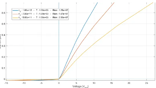
The plot of equation (58), using different plasma ion density (𝑛𝑝) is shown in Figure 3.9. The parameters used are the same of Figure 3.6 except for the length of the channel, the area of the junctions and the cross-section of the conductive channel (𝐴𝑐ℎ):

A1 = 10-5 Area of the D1 junction in m2

A2 = 10-3 Area of the D2 junction in m2

𝐴_𝑐ℎ = 10-5 _{Area of the ion channel in m}2

𝐿𝑐ℎ = 2*10-3 Length of the ion channel in m

𝜇_𝑒 = 100 , ( 𝜇_𝑒 > 𝜇_𝑝) Electron’s mobility in plasma in m2_{/(V s).}

In Figure 3.10, it is evident that the different area of the two junctions creates a rectification effect on the applied voltage. In Figure 3.9 is shown a plot, in the same condition of the previous one, but simulating different plasma temperatures (Ti=Te). The temperature variation of ions does not significantly affect the saturation regions of the probe.

Figure 3.9 - I-V Plot for the circuit in Figure 3.8. In this simulation A1 = 10-5 m2, A2 = 10-3 m2, 𝐴𝑐ℎ = 10-5

m2_{, 𝐿}

𝑐ℎ = 2*10-3 m, the other parameters are the same used in Figure 3.6. The different curves correspond to

(46)

44

Figure 3.10 - I-V Plot for the circuit in Figure 3.8. In this simulation A1 = 10-5 m2, A2 = 10-3 m2, 𝐴𝑐ℎ = 10

-5_m2_{, 𝐿}

𝑐ℎ = 2*10-3 m, the other parameters are the same used in Figure 3.6. The different curves correspond to

(47)

45

4 Ion Current Measurement Setup

A burner test bench was used to verify the model previously presented, and to evaluate the flame ion current in different combustion conditions. The combustible mixture with defined air to fuel ratios is obtained exploiting two controlled flows of air and propane (C3H8); 𝜙𝐴𝑖𝑟 and 𝜙𝐺𝑎𝑠, respectively. The mixture flow passes through a nozzle that impresses a rotation to the fluid to increase the flame stability (Figure 4.1). The combustion occurs after this nozzle, and the distance between the nozzle and the current probe (d) can be modified. To keep under control the temperature and avoid the overheating of the mechanical structure of the burner, a flow of cooling air around the burner is used. The probe is positioned before the mixing point of the cooling air to measure only the premixed contribution to the combustion. The exhaust gases produced by the combustion are tapped from the chimney, cooled, partially dehumidified and pumped to an exhaust gas analyser (this operation is usually referred to as ‘exhaust gas sampling’) to determine their composition in terms of Carbon Monoxide (CO), Nitric Oxides (NOx) and Oxygen (O2). This

measure will be used to be correlated with the ion density measured by the current probe.

(48)

46

As previously discussed, the quantity to be measured is the ion density in the gap between the two electrodes of the probe. From the electrical point of view, it is necessary to measure the current that flows in the probe through the ionic channel. This current, as discussed above, is due both to the ion channel characteristics and to the effect introduced by the Langmuir probe consisting of the two electrodes.

The characteristics of the signal to be measured, used for the design of the ion-current measurement instrument described hereafter, were obtained both from data reported in the literature and from preliminary tests on test burners, which made it possible to estimate both the dynamics and the frequency band of the expected signal in different operating conditions, and its statistical properties. These aspects are discussed in detail in the remainder of the paragraph.

(49)

47

Let us discuss about two possible measurement solutions that take advantage of a constant voltage (DC) or an alternate voltage (AC) excitation.

The instrument realized to measure the ion current generates the excitation signal and measures the current that flows through the electrodes. The structure of the instrument is shown in Figure 4.3, and two pictures of the instrument are shown in Figure 4.4 and Figure 4.5. The device is based on a microcontroller (STM32L432) embedding a 12-bit digital to analog converter (DAC), that is used to generate the waveform signals used to excite the current probe. The excitation signal can be a DC, a sinusoidal, a rectangular, or a triangular waveform. The signal shape, together with its amplitude and frequency, can be set by a serial interface and a Modbus® protocol. The signal generated by the DAC is amplified8_{up to a maximum of ±19𝑉 and, by a shunt resistor, is applied}

to the current probe. The shunt resistor is used to measure the current due to the presence of the ion channel. The voltage across the resistor is amplified by a differential stage9_{and adapted to the}

microcontroller 12-bit ADC dynamics by an analog front end. The acquired signal is processed, and the root mean square value in the period of the excitation waveform is calculated and made available on the serial Modbus® present on the STM32L432 module.

8_{The amplifier is based on an OPA454 operational amplifier used to drive a class B amplifier}

stage based on TIP2955 and TIP3055 transistors.

9_{The differential amplifier has been realized using a standard instrumentation amplifier layout}

(50)

48

Figure 4.3 - Measurement instrumentation block diagram.

Figure 4.4 – A picture of the measurement instrument prototype.

(51)

49

To debug the system, and to perform other more accurate measurements, the signal coming from the ion current probe can be also acquired using an external acquisition board, connected to a PC, which allows to perform more accurate and larger-bandwidth signal acquisitions.

The external acquisition board (NI-DAQ-6251) was used to sample the large bandwidth signal using a sampling frequency up to 1.25 MS/s. Using this setup, a preliminary analysis on the ion current signal has been performed to verify the expected signal bandwidth. From this analysis, the ion current signal is expected [30] to be limited in the bandwidth from 0 to 1kHz. The microcontroller ADC sampling frequency and the anti-aliasing filter in the analog front end have been designed to correctly acquire this signal bandwidth.

The probe electrical connection setup is shown in Figure 4.6: the inner part of the spark plug, that is the electrode with the smaller area, is connected to the positive side of the excitation voltage generator.

Figure 4.6 . Probe electrical connection: The voltage generator V and the current meter I represent the power amplifier and the current sensing reported in Figure 4.3, respectively.

(52)

50

Let us now introduce some considerations about the selection of the probe excitation signal. For this purpose, we assume, as a first approximation, that the measured ion current is determined only by the resistance of the channel (Figure 4.7)10_{. In Figure 4.7, V represents the excitation voltage}

whereas the capacitance C includes the parasitic capacitance of the conditioning electronics, mainly due to the cable capacitance (the coaxial cable used to limit interferences introduces a capacitance of approximately 100 pF/m).

Figure 4.7 - Equivalent simplified circuit of the current probe connected to the conditioning electronics. Rs is the current sensing resistor shown in Figure 4.3.

Considering Figure 4.7 it is possible to derive the expression of the current measured by the instrument (Is):

𝐼_𝑠 = 𝑉𝑠 𝑅_𝑠 =

𝑉

𝑍_𝑒𝑞+ 𝑅_𝑠 (62)

10_{This assumption is not generally valid, as it will be cleared in what follows, but allows for a}

(53)

51

Where Zeq is the equivalent impedance due to Rion and C, and Rs is the shunt resistor of Figure 4.3.

𝑍𝑒𝑞 =

𝑅_𝐼𝑜𝑛

1 + 𝑗𝜔𝑅𝐼𝑜𝑛𝐶 (63)

The equation (62) can be written as:

𝐼_𝑠 = 𝑉 𝑅_𝐼𝑜𝑛

1 + 𝑗𝜔𝑅𝐼𝑜𝑛𝐶 + 𝑅𝑠

(64)

From equation (64) it is evident that increasing the excitation frequency, the parasitic capacitance of the cable reduces the sensitivity of the current to ion resistance variations.

4.1 DC Measurements

DC measurements are performed by applying a constant voltage to the probe, which is proportional to the electric field applied between the electrodes. The optimal choice set up is to maximise the electric field applied across the channel without reaching the saturation electric field, as discussed in section 2.3.2.

From equation (64), if a DC excitation is considered (𝜔 = 0), the expression of the current becomes:

𝐼𝑠 = 𝑉 1 𝑅𝐼𝑜𝑛+ 𝑅𝑠

𝑖𝑓 𝜔 = 0 ₍₆₅₎

and a good sensitivity to the resistance of the ionic channel can be achieved. Unfortunately, DC measurements have a drawback that is experimentally verified: when using the spark plug, or any other electrode, the ion sensor output under DC polarization, in general after a few hours of

Ion current and exhaust gas composition measurements for combustion monitoring

DEPARTMENT

OF

INFORMATION

ENGINEERING

AND

MATHEMATICS

Doctor of Philosophy program in

INFORMATION ENGINEERING AND SCIENCE

Ion current and exhaust gas composition

measurements for combustion monitoring

Cycle XXXIII

a.a. 2019/2020

1

Table of Contents

2

3

4

1. Introduction

5

6

7

1.1 Contributions

8

9

2. Combustion Control: the possible role of ion

density measurements

10

11

2.1 Ion Current Measurement: State of the art

12

2.2 Ion Current theoretical background

13

14

15

16

17

2.3 Ion Channel

18

19

2.3.1

Small External Electric Field Assumption

20

21

2.3.2

Strong External Electric Field Assumption (Saturation)

2.4 A Numerical Model for the Burner

22

23

24

25

3 Current Probe Model

26

27

3.1 Ions probe physical background [23] [28]

28

29

30

3.1.1

Electron current

31

32

(36)

33

3.1.2

Ion current

34

35

3.1.3

I-V Model

36

37

3.1.4

Debye length

38

39

40

3.2 Ions probe equivalent circuit.

41

42