Aalborg Universitet
CLIMA 2016 - proceedings of the 12th REHVA World Congress
Heiselberg, Per Kvols
Publication date: 2016
Document Version
Publisher's PDF, also known as Version of record
Link to publication from Aalborg University
Citation for published version (APA):
Heiselberg, P. K. (Ed.) (2016). CLIMA 2016 - proceedings of the 12th REHVA World Congress: volume 8. Aalborg: Aalborg University, Department of Civil Engineering.
General rights
Copyright and moral rights for the publications made accessible in the public portal are retained by the authors and/or other copyright owners and it is a condition of accessing publications that users recognise and abide by the legal requirements associated with these rights. ? Users may download and print one copy of any publication from the public portal for the purpose of private study or research. ? You may not further distribute the material or use it for any profit-making activity or commercial gain
? You may freely distribute the URL identifying the publication in the public portal ? Take down policy
If you believe that this document breaches copyright please contact us at [email protected] providing details, and we will remove access to the work immediately and investigate your claim.
Comparative Analysis of Thermal Unit Control Methods for
Sustainable Housing Applications
Cihan Turhan #1, Silvio Simani *2, Ivan Zajic &3, Gülden Gökçen Akkurt $4 #1
Mechanical Engineering, Izmir Institute of Technology Gulbahce Campus, Urla - 35430 Izmir, TURKEY
*2
Department of Engineering, University of Ferrara Via Saragat 1E. 44123 Ferrara (FE), ITALY
&3
Control Theory and Applications Centre, Coventry University Coventry, UK
$4
Energy Engineering Program, Izmir Institute of Technology Gulbahce Campus, Urla - 35430 Izmir, TURKEY
Abstract
This study aims to develop different control strategies for application to nonlinear model of a thermal unit and compare their performances as an advanced thermal control methods for HVAC applications of sustainable buildings. The mathematical description of thermal unit was obtained exploiting a data-driven and physically meaningful nonlinear continuous-time model, which represents a test-bed used in passive air conditioning for sustainable housing applications. The presented controller strategies use both inside temperature and air flow control in the thermal unit. The proposed control schemes were assessed with extensive simulations and Monte-Carlo analysis in the presence of modelling and measurement errors. The contribution of this work consists of providing an application example of the design and testing through simulations, of a data-driven thermal unit control. Furthermore, this study provides an insight into different control strategies in air conditioning systems and helps the practitioners and HVAC learners to design proper controller solutions.
Keywords - thermal unit; modelling and simulation for control; advanced control design; artificial intelligence; nonlinear control design
1. Introduction
The distribution of energy consumption in Europe households was as follows in 2015: 50% for air conditioning, 13% for water heating and 12% for lighting and electric appliances [1]. Air conditioning systems provide buildings with heating/cooling functions and thermal comfort parameters including relative humidity and temperature. Thermal Units (TUs) play an essential role for supplying treated air with specified temperature to the conditioned space in the buildings. Hence, it is fundamental to understand the system behaviour of TUs in order to decrease energy consumption and achieve thermal comfort in buildings [2].
The TU system is a typical nonlinear time-variable multivariable system with disturbances in the view of control [3]. Many control methods use traditional controllers like on-off controllers, Proportional,Integral and Differential (PID) or Proportional and Integral (PI) regulators [4]. These controllers are simple and low-cost, however, sometimes are not able to produce accurate results. Moreover, the TU system has bilinear terms like temperature and mass flow rate, hence, advanced controllers must be replaced for an improved thermal comfort and a lower energy consumption. To overcome the problems stated above, Artificial Intelligent (AI) based controllers, namely, Artificial Neural Network (ANN), Fuzzy Logic (FL), Adaptive Neuro-Fuzzy Inference System (ANFIS) and Model Predictive Controllers (MPC) have been applied for trying to achieve more comfortable environments in buildings [5]. FL controllers are based on human knowledge of the system behaviour and require no mathematical modelling. In addition to FL controllers, some authors studied ANN controllers to maintain a better thermal comfort for heating purposes [3]. Although ANN controllers presents interesting features such as learning, adaptation, fault-tolerance and generalization, some researchers studied more efficient control techniques based on ANFIS tool [5] and MPC for temperature control of buildings [1]. Note finally that many studies proved thermal comfort and energy efficiency using AI control techniques, however the performance of the AI based-methods were not compared with extensive simulations in most of them. This paper aims to design different control techniques with application to a nonlinear TU model developed by Ref. [6]. Another objective of the paper is to highlight the potential application of the proposed control strategies to real air conditioning systems and help the practitioners and HVAC learners to design better controllers in their work. To this aim, the simulations and comparisons have been implemented in the Matlab and Simulink environments.
2. Thermal Unit Model
The TU is part of a larger test-bed system for testing and numerical modelling of phase change materials (PCM) used in the passive air
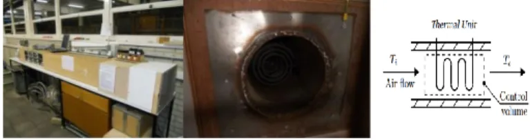
conditioning for sustainable housing applications. The speed and temperature of air passing around the tested PCM can be freely regulated to meet the demanded test environmental conditions, as shown in Fig. 1. The air is conditioned by means of the considered heating element which is in a down stream series connection with a cooling unit.
Fig. 1. The TU test-bed and schematic description of the TU
For the system identification purposes the following system inputs are considered: the measured inlet air temperature, denoted Ti [K], and the air velocity, denoted v [m/s]. The outlet air temperature, denoted To [K], is the system output. The data acquisition experimental set-up has been designed such that the supplied power, denoted q [W], to the heating element is constant with the average reading of q= 830 [W]. The measurements of v, Ti and To are taken from the centre of the cross sectional area of the supply duct.
The energy balance equations of the TU, the control volume of air surrounding the TU and the adjacent duct walls can be expressed as:
Ch (dTh(t)/dt)= q(t) – (UA)h [Th(t) – To (t)] (1)
0 = (UA)h [Th(t) – To (t)] - v(t) ρa Aa ca [To(t)- Ti(t)]-
(UA)int[To(t)-Tw(t)] (2)
Cw (dTw(t)/dt)= (UA)int [To(t)- Tw(t)] –
(UA)ext[Tw(t)-Ta(t)] (3) Here, Ch [J/K] is the thermal capacity of the heating element, Cw [J/K] thermal wall capacity (insulated plywood), ca [J/kgK] is the air specific heat capacity, Aa [m2] denotes the cross sectional area of the duct, ρa [kg/m3] is the air density. The heat transfer coefficient is denoted by U [J/m2K] while the product of the heat transfer coefficient and the efficient surface area, A [m2], through which the heat is transmitted is denoted by (UA)h [J/K] (when referred to the TU) (UA)int [J/K] (inner duct wall) and (UA)ext [J/K] (outer duct wall). The mean temperature of the heating element and wall temperature are denoted, respectively, by Th(t) [K] and Tw(t) [K]. In (2), it is assumed that the passing air has negligible thermal capacity, hence the
left hand side of the equation equals to zero. A standard thermocouple type K has been used to measure the air temperatures. The accuracy is around 1 °C for the whole measurement range. The airflow has been measured using a Hot Wire Thermo-anemometer with declared accuracy of 5%. For further detail of the TU model, please see Ref.[6].
3. Development of Control Logics for Thermal Unit
TU process, which is basically a MISO system, has several nonlinear components like temperature and air flow. The general description of the dynamic model of TU can be expressed by the nonlinear dynamic function
P:
y= P (u,t) (4)
Here, y is the process output, u are the inputs and t is the time. The control strategy applied to the TU should determine the control input such that the controlled process is able to track a given reference r(t) [6].
The control input is represented by the air flow input temperature
u(t)= Ti, and the measured output is y(t) = To. In building HVAC control systems, bilinear terms are the most dominant ones. (Temperature)X(mass flow rate ) can be given as an example in HVAC systems. Therefore, mass flow rate is considered as a measured disturbance, d. The data contain the inlet temperature, the air flow and the outlet temperature were obtained from the experimental work. The measurement errors were added to the the temperature and air flow signals.
The PID controller has been commonly used in many HVAC system applications [4,5]. The PID controller produces promising results based on the computation of the error e(t) between the desired and the measured values of the output, ie. e(t) =r(t)- y(t).
The continous-time control law of the PID regulator is described by (5):
u(t)= Kp e(t) + Ki∫ 𝑒(𝜏)𝑑𝜏
𝑡
0 + Kd
𝑑𝑒(𝑡)
𝑑𝑡 (5)
where Kp, Ki, Kd are the PID proportional, integral and derivative gains, respectively. The control of the TU is therefore carried out by a PI regulator (5) as shown in Fig. 2.
Fig.2. Block diagram of the TU system controlled by the PI regulator
In FL controller, controller actions are implemented in the form of if-then-else statements [7]. The controller design approach relies on the identification of transparent rule-based Takagi-Sugeno (TS) fuzzy models using an ANFIS tool implemented in the Simulink toolbox [8].
Fig.3. Block diagram of the TU system controlled by the ANFIS fuzzy regulator
The TS fuzzy model consists of a set of rules Ri, where the consequents are deterministic functions fi:
Ri= IF x is Ai THEN yi= fi(x) (6) where i= 1, 2, ……, K. Here, K is the number of clusters. The term x describes the antecedent variables, whilst yi represents the consequent output. The fuzzy set Ai of the ith rule is represented with a multivariable membership function in (7):
µ Ai (x)→ [0,1] (7) Note finally that the final output y of the TS fuzzy model is represented as:
y = ∑ µ𝐴𝑖(𝑥)𝑦𝑖 (𝑥)
𝐾 𝑖=1
This paper also considers an effective approach called Fuzzy Modelling and Identification (FMID) toolbox developed in the Matlab environment. Fuzzy models are automatically generated from the measurements by a comprehensive methodology described e.g. in Ref. [9]. The system relies on the identification of rule-based fuzzy models and using the input-output data acquired from the controlled process. The method employs Gustafson-Kessel clustering method to divide the data into subsets with a common local linear behaviour. The identified fuzzy controller requires a proper model structure n and a number of clusters K. The developed method provides the parameters ai, bi and the estimation of the membership functions µAi of the optimal controller minimising the tracking error e(t) which is the difference between the reference signal r(t) and the measured output y(t).
Fig.4. Block diagram of the TU system controlled by the FMID fuzzy regulator
The adaptive control method is based on the on-line identification of a second order discrete-time transfer function of an ARX time-varying model described in (9):
G (z) = 𝑏1 𝑧−1 +𝑏2 𝑧−2
1+ 𝑎1 𝑧−1 +𝑎2 𝑧−2 (9) where z represents the unit advance operator and parameters are recursively estimated at each sampling time tk= kT where k is the number of samples and T is the sampling interval. The on-line identification employs Recursive Least Squares Method (RLSM) with adaptive directional forgetting.
Fig.5. Block diagram of the TU system controlled by the adaptive regulator
Model Predictive Controller (MPC) predicts the future nonlinear system behaviours and generates a control vector over the prediction horizon. The controller implements current sampling time but optimises a finite time-horizon. The main advantage of MPC over PID controllers is predictive ability.
The MPC obtains control signals by minimizing objective function (J) as:
J = ∑𝑘+𝑁𝑝𝑘 𝑤 [𝑦𝑘] ( rk – yk )2 + ∑𝑘+𝑁𝑐𝑘 𝑤 [𝑢𝑘] Δ 𝑢𝑘2 (10)
where w[yk] is the weighting coefficient reflecting the relative importance of the monitored output, w[uk] is the weighting coefficient penalising relative big changes in uk and Δ uk = uk - uk-1 , Np represents the prediction horizon and Nc is the control horizon.
Fig.6. Block diagram of the TU system controlled by the MPC
The study recalls different control strategies including standard PI controller as well as AI techniques, such as FL, adaptive, model predictive controllers, which are used for the regulation of the outlet temperature of the TU system. The results of each regulator are compared in terms of Mean Sum of Squared Errors (MSSE %), as shown in (11):
MSSE % = 100 √∑ (𝒓𝒌−𝒚𝒌)𝟐
𝑵 𝒌=𝟏
∑𝑵𝒌=𝟏(𝒓𝒌)𝟐 (11)
4. Simulation Results and Discussion
Most of the HVAC systems use classical PID regulators , the control of the TU is therefore carried out by a PI regulator as shown in Fig. 2.
The optimal proportional and integral gains are determined using the automatic PID tuning procedure and settled to Kp=2 and Ki=3, respectively. The PI controller has a settling time (Ts) of 2.17, with an overshoot (S%) of 36.14. These values are computed by applying a step change in the reference output temperature from 39 oC to 40 oC. The tracking error ,achieved by using (5), is MSSE%= 1.65 (Fig.7).
Fig.7. Outlet temperature controlled by the PI regulator
Classical controllers, such the PI controller used for the TU system, are robust and allow accurate tuning, hence have the benefit of quite straight- forward implementation. Nevertheless, the control laws are not efficient and can lead possible high maintenance costs. Therefore, the authors of this paper appraise advanced controllers in order to reduce energy consumption while maintaining the thermal comfort. To this aim, the PI regulator of TU system represents the reference controller for the generation of the data used by the advanced controller set-up. Fuzzy identification method is used to derive the models of the controllers by exploiting the so-called model reference control approach as described in Ref. [10]. The TS fuzzy controller , as described in previous section, is derived with the ANFIS tool, a sampling interval (T) of 0.1 s is exploited . Fig. 3 depicts the fuzzy regulator, which has a number of K=3 of Gaussian membership functions, with a number of delayed inputs and output n=1. The antecedent vector of the ANFIS controller is x= [ek, ek-1,uk-1]. Table 1 highlights the achieved performance of the regulator obtained with the ANFIS tool. In this case, the settling time is Ts = 2.21, with an overshoot of S%=38.22 and a MSSE%= 1.07(Fig.8). 0 200 400 600 800 100 0 120 0 14 00 160 0 180 0 22 24 26 28 34 36 38 40 Time (s) r(t ) & y (t ) [o C] Temperature outlet 32 30 r y (t) & (t) [°C] Reference PI regulator
Fig.8. Outlet temperature controlled by the ANFIS regulator
In this work, a second fuzzy regulator was implemented by using the same data from the standard PI controller of the TU system. The regulator uses the FMID tool which predicts the optimal shapes of the membership functions of µA . Fig. 4 shows the implementation of the fuzzy regulator with a number of clusters K=3, number of delays n=2 and the antecedent vector of x= [ uk-1,uk-2,rk,rk-1,yk,yk-1] . The reference signal is tracked with a
MSSE% of 1.14. In this case, the settling time is Ts= 3.98 s with a maximum overshoot S% of 41.65 (Fig.9).
Fig.9. Outlet temperature controlled by the FMID regulator
On the other hand, an adaptive controller was developed by using the online procedure recalled in previous section. Fig.5 shows the block diagram of the adaptive controller used for TU system. Time-varying parameters have been settled to δ = ω = 1 which are defined as damping factor and natural frequency, respectively. The settling time of the adaptive controller is Ts=3 .65 s with a maximum overshoot S% of 40.18 and the tracking error of MSSE%= 1.18 (Fig.10).
0 200 400 600 800 100 0 1 20 0 140 0 160 0 180 0 22 24 26 36 38 40
Tout outlet temperature
Time (s) r(t ) & y( t) [o C] 28 30 3 2 34 r y (t) & (t) [°C] ANFIS Regulator Reference 0 200 400 600 800 100 0 120 0 140 0 160 0 180 0 2 2 2 4 2 6 2 8 3 6 3 8 4 0 42
Tout outlet temperature
Time (s) 3 0 32 3 4 r y (t) & (t) [°C] FMID Regulator Reference
Fig.10. Outlet temperature controlled by the adaptive regulator
With reference to the MPC strategy recalled in previous section, the MPC were developed for the TU system (Fig.6). Note that the MPC of the TU uses a prediction horizon of Np=10 and a control horizon of Nc=2. The weighting parameters were selected as wyk= 0.1 and wuk=1 in order to reduce abrupt changes of the control input that would increase the energy consumption. In this case, the settling time is Ts= 1.85s and the overshoot is
S%=35.51 with a tracking error of MSSE%=0.41 (Fig.11).
Fig.11. Outlet temperature controlled by the MPC
Table 1 depicts the comparison of the results achieved from different regulators used for the TU system in terms of settling time (Ts), overshoot (S%) and tracking error (MSSE%).
Table 1. Comparison of the proposed controller performance in terms of MMSE, Settling Time and Overshoot Controller Type Settling time (Ts) Overshoot (S%) MMSE% (Nominal value) PI 2.17 36.14% 1.65 % ANFIS 2.21 38.22% 1.07% FMID 3.98 41.65% 1.14% Adaptive 3.65 40.18% 1.18% MPC 1.85 35.51% 0.41 % 0 2 00 400 600 800 100 0 120 0 140 0 160 0 180 0 22 24 26 28 30 32 34 36 38 40
Tout outlet temperature
Time (s) r y (t) & (t) [°C] Reference Adaptive Regulator 0 200 400 600 8 00 1 000 120 0 140 0 160 0 180 0 22 24 26 28 30 32 34 36 38 40 Tim e (s ) Tout outlet temperature
r y (t) & (t) [°C] Reference MPC
The MPC implementation is able to track the reference signal very accurately, thus maintaining the thermal comfort for energy-efficient buildings. In addition, ANFIS controller has good values of settling time, overshoot and the tracking error compared to the other ones. The PI regulator leads to the second best settling time as it uses auto-tuning in the Simulink environment in order to optimise parameters.
5. Robustness evaluation
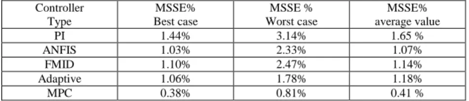
This section presents further simulation results and the robustness features of the proposed controllers with respect to parameter variations. The robustness evaluation was performed according the approach already described in detail in Ref. [11]. The Monte–Carlo (MC) tool is useful as the control strategy performances depend on the error magnitude due to the model approximation and uncertainty, as well as on input–output measurement errors. The MC analysis describes TU model parameters as Gaussian variables with standard deviations of 20% corresponding to the maximal error values. Therefore, for performance evaluation of the control schemes, the best, average, and worst values of the MSSE% performance index were computed, and experimentally evaluated with 500 Monte–Carlo runs, as shown in Table 2.
Table 2. Comparison of the performances in terms of MSSE% Controller Type MSSE% Best case MSSE % Worst case MSSE% average value PI 1.44% 3.14% 1.65 % ANFIS 1.03% 2.33% 1.07% FMID 1.10% 2.47% 1.14% Adaptive 1.06% 1.78% 1.18% MPC 0.38% 0.81% 0.41 %
Note finally that, MC analysis is an effective tool in presence of uncertainty and modelling errors and can be used for testing the suggested control methods for TU system.
6. Conclusion
In this paper, different control schemes varying from PI regulator to MPC were implemented to a nonlinear TU model, which represents a part of a larger system used for PCM in passive air conditioning for sustainable housing applications andthe results were compared with the measurements. The feasibility and robustness issues of the proposed tools were demonstrated experimentally. The proposed control schemes were assessed with extensive simulations and Monte-Carlo analysis in the presence of modelling and measurement errors. Some final comments can be drawn
here. The achieved results showed that AI-based controllers can be successfully used for the regulation of the temperature of TU systems. Compared to the classical control approach, the TU model can be well described by advanced control techniques. MPC presented the best values of settling time, maximum overshoot and tracking error. However, the MPC strategy requires extra effort to find a suitable construction. The fuzzy-based controllers were fuzzy-based on the learning accumulated from off-line simulations but it is time-consuming to train the model properly. MC simulation tool was effective to facilitate the validation of the considered control schemes for application to real HVAC systems.
In this paper, the temperature of air and the air flow were taken into account; future works will focus on trying to extend the developed controllers to control more thermal comfort parameters, such as relative humidity, air flow and temperature. Moreover, the real evaluation of the MC analysis will be presented.
7. References
[1] D.Lindelof, H.Afshari, M.Alisafaee, J.Biswas, M.Caban, X.Mocellin, J. Viaene. Field tests of an adaptive, model-predictive heating controller for residential buildings. Energy and Buildings. 99 (1) (2015) 292-302.
[2] P.M Ferreira, A.E. Ruano, S. Silva, E.Z.E Conceiçao. Neural networks based predictive control for thermal comfort and energy savings in buildings. Energy and Buildings. 55 (2012) 238-251.
[3] H. Mirinejad, S.H. Sadati, M. Ghasemian, H. Torab. Control techniques in Heating,Ventilating and Air Conditioning(HVAC) systems. Journal of Computer Science. 4 (9) (2008) 777-783.
[4] Q.G.Wang, T.H.Lee, H.W.Fung, Q.Bi, Y.Zhang. PID tuning for improved performance. Control System Technology, IEEE Transactions. 7 (4) (1999) 457-465.
[5] J.Moon, S.K. Jung, Y.Kim, S.H.Han. Comparative study of artificial intelligence-based building thermal control-Application of fuzzy, adaptive neuro-fuzzy inference system and artificial neural network. Applied Thermal Engineering. 31 (14-15) (2011) 2422-2429. [6] I.Zajic, M. Iten, K.J. Burnham. Modeling and data-based identification of heating element in continuous domain. Journal of Physics:Conference Series. 570 (1) (2014) 012003.
[7] M.M Gouda, S.Danaher, C.P. Underwood. Thermal comfort based fuzzy logic controller.Building Services Engineering Research & Technology. 22 (2001) 237-253. [8] J.S.R. Jang. ANFIS: Adaptive-Network-based Fuzzy Inference System. IEEE Transactions on Systems, Man &Cybernetics .23 (3) (1993) 665-684.
[9] R. Babuska. Fuzzy Modeling for Control. 1998, Kluwer Academic Publishers, Boston USA.
[10] V. Bobal, J.Böhm, J. Fessl, J. Machacek. Digital Self-Tuning Controllers: Algorithms, Implementation and Applications. Advanced Textbooks in Control and Signal Processing. 2005, 1st Edition, Springer.
[11]R. J. Patton, F. J. Uppal, S. Simani, and B. Polle, “Robust FDI applied to thruster faults of a satellite system,” Control Engineering Practice, vol. 18, pp. 1093–1109, September 2010. ACA’07 – 17th IFAC Symposium on Automatic Control in Aerospace Special Issue. Publisher: Elsevier Science. ISSN: 0967–0661. DOI: 10.1016/j.conengprac.2009.04.011.