Improving
CtxMatch by means of
grammatical and ontological knowledge – in order
to handle attributes
S. Zanobini
Contents
1 Introduction 2
2 Our approach 4
3 CtxMatch 7
3.1 CtxMatch: the general algorithm . . . 7
3.1.1 Building the contextual meaning . . . 9
3.1.2 Comparing the concepts . . . 10
3.2 Semantic coordination of HCs . . . 11
3.2.1 HC–specific functions for build-ctx-meaning . . . 11
3.2.2 HC–specific functions for semantic–comparison . . . . 14
4 Improving HC-CtxMatch 17 4.1 The general approach . . . 17
4.1.1 Using DL . . . 18
4.1.2 Grammatical knowledge . . . 20
4.1.3 Ontological knowledge . . . 21
4.2 Building formulas . . . 22
4.2.1 Individuating the functionality of a node . . . 22
4.2.2 Individuating the semantic atoms . . . 24
4.2.3 Building the formula . . . 25
4.3 Handling the ambiguity . . . 28
4.3.1 No relation between two atoms . . . 29
4.3.2 Multiple relations between two atoms . . . 30
4.3.3 Bidirectional relations . . . 31
4.3.4 Multiple relations with ancestors or siblings . . . 31
4.4 Catalogues – Cat-CtxMatch . . . 32
Chapter 1
Introduction
With the development of WWW, one of the more recent issue is the problem of enabling machines to exchange meaningful information/knowledge across appli-cations which (i) may use autonomously developed models of locally available data (local models), and (ii) need to find a sort of agreement on what local models are about to achieve their users’ goals. This problem can be viewed as a problem of semantic coordination1
, defined as follows: (i) all parties have an interest in finding an agreement on how to map their models onto each others, but (ii) there are many possible/plausible solutions (many alternative mappings across local models) among which they need to select the right, or at least a sufficiently good, one.
In environments with more or less well-defined boundaries, like a corpo-rate Intranet, the semantic coordination problem can be addressed by defining and using shared models (e.g., ontologies) throughout the entire organization2
. However, in open environments, like the Semantic Web, this “centralized” ap-proach to semantic coordination is not viable for several reasons, such as the difficulty of “negotiating” a shared model of data that suits the needs of all parties involved, the practical impossibility of maintaining such a model in a highly dynamic environment, the problem of finding a satisfactory mapping of pre-existing local models onto such a global model. In such a scenario, the prob-lem of exchanging meaningful information across locally defined models seems particularly tough, as we cannot presuppose an a priori agreement, and there-fore its solution requires a more dynamic and flexible form of “peer-to-peer” semantic coordination.
In a recent paper ([5]), we address an important instance of the problem of semantic coordination, namely the problem of coordinating hierarchical clas-sifications (HCs). HCs are structures having the explicit purpose of organiz-ing/classifying some kind of data (such as documents, records in a database,
1
See the introduction of [2] for this notion, and its relation with the notion of meaning negotiation.
2
But see [1] for a discussion of the drawbacks of this approach from the standpoint of Knowledge Management applications.
goods, activities, services) and are widely used in many applications. Examples are: web directories (see e.g. the GoogleTM
Directory or the Yahoo!TM
Directory), content management tools and portals (which often use hierarchical classifica-tions to organize documents and web pages), service registry (web services are typically classified in a hierarchical form, e.g. in UDDI), marketplaces (goods are classified in hierarchical catalogs), PC’s file systems (where files are typically classified in hierarchical folder structures).
In particular, we propose in [5] a logic–based algorithm, called CtxMatch, for coordinating HCs. It takes in input two HCs H and H0 and, for each pair
of concepts k ∈ H and k0∈ H0, returns their semantic relation3
.
With respect to other approaches to semantic coordination proposed in the literature, our approach is innovative in three main aspects: (1) we introduce a new method for making explicit the meaning of nodes in a HC (and in general, in structured semantic models) by combining three different types of knowledge, each of which has a specific role; (2) the result of applying this method is that we are able to produce a new representation of a HC, in which all relevant knowledge about the nodes (including their meaning in that specific HC) is encoded as a set of logical formulae; (3) mappings across nodes of two HCs are then deduced via logical reasoning, rather then derived through some more or less complex heuristic procedure, and thus can be assigned a clearly defined model-theoretic semantics.
In particular, the point (2) represents a new and relevant problem in NLP. In fact, despite the presence of a large literature addressing the problem of encoding natural language statements into logical formulas [6, 7, 8, 3], no approach has been proposed addressing the issues raised by point (2). The problem is relevant, because of the recent development of the WWW, where these kind of structures are widely used for representing domains. The goal of this paper is to define an improvement for the simple encoding process used in CtxMatch.
This paper proceeds as follow: in Chapter 2 we present the general approach followed in CtxMatch. In chapter 3 we analyze in detail the algorithm. In Chapter 4 we show a general problem afflicting CtxMatch and we propose a solution.
3
The relations we consider in this version of CtxMatch are: k is less general than k0
, k is more general than k0, k is equivalent to k0, k is compatible with k0, and k is incompatible
Chapter 2
Our approach
The approach to semantic coordination we propose in [5] is based on the intuition that there is an essential conceptual difference between coordinating generic ab-stract structures (e.g., arbitrary labelled graphs) and coordinating structures whose labels are taken from the language spoken by the community of their users. Indeed, the second type of structures give us the chance of exploiting the complex degree of semantic coordination implicit in the way a community uses the language from which the labels are taken. Most importantly, the status of this linguistic coordination at a given time is already “codified” in artifacts (e.g., dictionaries, but today also ontologies and other formalized models), which pro-vide senses for words and more complex expressions, relations between senses, and other important knowledge about them. Our aim is to exploit these ar-tifacts as an essential source of constraints on possible/acceptable mappings across HCs.
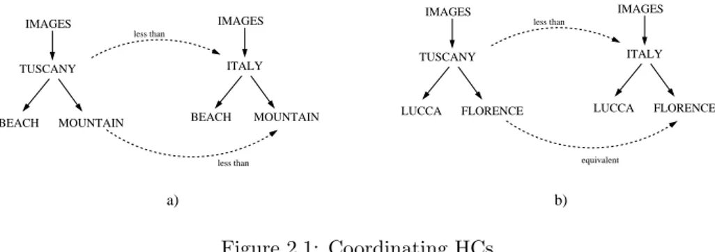
To clarify this intuition, let us consider the HCs in Figure 2.1, and suppose they are used to classify images in two multi-media repositories. Imagine we want to discover the semantic relation between the nodes labelled MOUNTAIN in the two HCs on the left hand side, and between the two nodes FLORENCE on the right hand side. Using knowledge about the meaning of labels and about the world, we understand almost immediately that the relation between the first pair of nodes is “less general than” (intuitively, the images that one would classify as images of mountains in Tuscany is a subset of images that one would classify under images of mountains in Italy), and that the relation between the second pair of nodes is “equivalent to” (the images that one would classify as images of Florence in Tuscany are the same as the images that one would classify under images of Florence in Italy). Notice that the relation is different, even though the two pairs of HCs are structurally equivalent. How do we design a technique of semantic coordination which exploits the same kind of facts to achieve the same results?
The approach we propose is based on three basic ideas.
1. Three levels of knowledge. First of all, exploiting the degree of coordination implicit in the fact that labels are taken from language requires
less than IMAGES IMAGES ITALY TUSCANY LUCCA FLORENCE LUCCA FLORENCE equivalent less than IMAGES MOUNTAIN IMAGES TUSCANY
BEACH MOUNTAIN BEACH ITALY
less than
a) b)
Figure 2.1: Coordinating HCs
to make explicit the meaning of labels associated to each node in a HC. We claim that this can be done only of we properly take into account three distinct levels of semantic knowledge:
Lexical knowledge: knowledge about the words used in the labels. For ex-ample, the fact that the word ‘image’ can be used in the sense of a picture or in the sense of personal facade, and the fact that different words may have the same sense (e.g., ‘picture’ and ‘image’);
Domain knowledge: knowledge about the relation between the senses of la-bels in the real world or in a specific domain. For example, the fact that Tuscany is part of Italy, or that Florence is in Italy;
Structural knowledge: knowledge deriving from how labels are arranged in a given HC. For example, the fact that the concept labelled MOUNTAIN classifies images, and not books.
Let us see how these three levels can be used to explain the intuitive reason-ing described above. Consider the mappreason-ing between the two nodes MOUNTAIN. Linguistic meaning can be used to assume that the sense of the two labels is the same. Domain knowledge tells us, among other things, that Tuscany is part of Italy. Finally, structural knowledge tells us that the intended meaning of the two nodes MOUNTAIN is images of Tuscan mountains (left HC) and images of Italian mountains (right HC). All these facts together allow us to conclude that one node is less general than the other one. We can use similar reasoning for the two nodes FLORENCE, which are structurally equivalent. But exploiting domain knowledge, we can add the fact that Florence is in Tuscany (such a relation doesn’t hold between mountains and Italy in the first example). This further piece of domain knowledge allows us to conclude that, beyond structural similarity, the relation is different.
2. Encoding the concepts. This analysis of meaning has an important consequence on our approach to semantic coordination. Indeed, unlike all other approaches we know of, we do not use lexical knowledge (and, in our case, domain knowledge) to improve the results of structural matching (e.g., by adding
synonyms for labels, or expanding acronyms). Instead, we combine knowledge from all three levels to build a new representation of the problem, where the meaning of each node is encoded as a logical formula, and relevant domain knowledge and structural relations between nodes are added to nodes as sets of axioms that capture background knowledge about them.
3. Problem of satisfiability. This, in turn, introduces the third innovative idea of our approach. Indeed, once the meaning of each node, together with all relevant domain and structural knowledge, is encoded as a set of logical formulae, the problem of discovering the semantic relation between two nodes can be stated not as a matching problem, but as a relatively simple problem of logical deduction. Intuitively, determining whether there is an equivalence relation between the meaning of two nodes becomes a problem of testing whether the first implies the second and vice versa (given a suitable collection of axioms, which acts as a sort of background theory); and determining whether one is less general than the other one amounts to testing if the first implies the second. As we will say, in the current version of the algorithm we encode this reasoning problem as a problem of logical satisfiability, and then compute mappings by feeding the problem to a standard SAT solver.
Chapter 3
CtxMatch
In this chapter, we propose (i) a general algorithm, called CtxMatch, for dis-covering (semantic) relationships across distinct and autonomous generic struc-tures (section 3.1) and (ii) a specific algorithm specializing the algorithm to the discovering of mappings across hierarchical classifications (section 3.2).
3.1
CtxMatch: the general algorithm
The general framework described in Chapter 2 can be used for discovering rela-tions between any structures labelled with natural language. In this section, we introduce the structure and purpose independent part of the algorithm, namely the steps that do not depend on the use nor on the type of structure. This generic algorithm must be obviously enriched with specific structure and pur-pose dependent functions, i.e. with different functions for each particular type and use of the structures we want to match. In Section 3.2 we present the specific functions we use to match Hierarchical Classifications, i.e., tree-like structures used for classifying documents.
To make things clearer, imagine the following scenario: an agent A (the seeker) has a set of documents organized into a tree–structure. To collect new documents, he can send a query to a provider (an agent B). In our approach, the agent can formulate the query using his own structure: for example, imagine that seeker A uses the structure on the right-hand side of Figure 2.1.b to classify his documents. Then, he can select node FLORENCE to formulate the query ‘Images of Florence in Italy’. Furthermore, imagine that the provider employs the left-hand structure in Figure 2.1.b. After receiving the query, he has the following tasks: (i) to interpret the query he receives, (ii) to find semantic relations holding between the query and his structures, and (iii) to return relevant documents (if any). In particular, in this paper we focus on the tasks (i) and (ii).
The algorithm needs two inputs:
query Q: A seeker sends a query composed by a node fl in a structure FS. It means simply that the seeker wants to find nodes semantically related to the
node fl in FS;
context C: The context is composed by the three elements of the local knowl-edge, namely a structure LS, a lexicon LL and an ontology LO. The context is the target of the query1
.
The main goal of the algorithm CtxMatch is to find the semantic relations between node f l in the query Q and all the nodes belonging to the local structure LS in the context C. For the sake of simplicity, in this paper we focus on the procedure for matching the node f l in the query with a single nodes ll in the context C. Therefore, for this simplified version of CtxMatch, we add a third element in the input: a label ll of the structure LS. The output of the algorithm will simply be the semantic relation holding between the two nodes.
The algorithm also employs a data–type ‘concept’ hφ, αi, constituted by a pair of logical formulas, where φ approximating the individual concept repre-sented by a node of a structure and α expressing the relations between the current individual concept and other individual concepts in the structures (local relevant axioms). E.g., the formulas associated with the node labeled FLORENCE in rightmost structure in Figure 2.1.b will approximate the statements ‘images of Florence in Italy’ (the individual concept) and ‘Florence is in Italy’ (the local relevant axiom).
Algorithm 3.1 CtxMatch(Q, C, ll)
.query Q = hf l, F Si where f l is the foreign term F Sis the foreign structure
.context C = hLS, LL, LOi where LS is the local structure LLis the local lexicon LOis the local ontology
.label ll is the label of the local node to be matched
VarDeclarations context QC;
concept hφ, αi, hψ, βi; .concepts are pairs of formulas
relation R;
1 QC←hF S, LL, LOi;
.QCrepresents the virtual query context
2 hφ, αi← build–cxt–meaning(f l, QC);
3 hψ, βi← build–cxt–meaning(ll, C);
.compute the concepts expressed by label ll and f l
4 R← semantic–comparison(hφ, αi, hψ, βi, LO);
.Rrepresents the semantic relation between the two concepts
5 ReturnR;
In line 1, CtxMatch first builds the ‘virtual’ query–context QC. The reason of it is that we want the query Q to be locally interpreted within the local lexicon and ontology. An important consequence is that the relation returned by the
1
We call context the ensemble of the three levels of knowledge because they express the local representation that an agent has of a portion of the world.
algorithm is directional: it expresses the relation holding between the two nodes from the provider’s point of view. Indeed, the seeker could have different lexicon and ontology and could calculate different relation for the same nodes.
Then, line 2 builds a concept, i.e. a pair of logical formulas, approximating the meaning of the node f l in the virtual context QC. Line 3 similarly builds the concept for the node ll in the local context C. Finally, line 4 computes the semantic relation between the two concepts. The following two subsections describes in more detail this two top-level operations, implemented by the func-tions build–ctx–meaning and semantic–comparison.
3.1.1
Building the contextual meaning
This step has the task of building the concept expressed by a generic node t in a generic context GC. Before analyzing the corpus of the algorithm, it’s important to focus our attention on the array of senses SynS. A synset (set of synonyms) is a set of senses, i.e. of concepts, expressed by an expression of the natural language2
. For example the word ‘Florence’ has, in WordNet, two senses (i.e. it may express two different concepts): ‘city of Tuscany’ and ‘town of South Caroline’. The array SynS records these senses, so that, for example, SynS[Florence] is the synset containing the two senses above, while SynS[Florence][0] is the first of the two senses.
Algorithm 3.2 build–ctx–meaning(GC, t)
.context GC = hT, L, Oi, where T is a structure Lis a lexicon Ois an ontology
.label t is a generic label
VarDeclarations
sense SynS[][] .array of senses
structure F formula α, η
1 F← determine–focus(t, T );
.the focus F is a substructure of T
2 for each label e in F do
3 SynS[e]← extract–synset(e, L);
.extracts the senses associated to each label in the structure F
4 for each label e in F do
5 SynS[e]← filter–synset(F, O, SynS, e);
.unreasonable senses are discarded
6 δ← individual–concept(t, SynS, F, O);
7 η← extract–local-axioms(F, SynS, O);
8 Returnhδ, ηi;
Let us now look at the algorithm. Line 1 determines the focus of a node t, i.e. the subgraph of the structure T useful to extract the meaning of t. This step
2
is performed essentially for efficiency reasons, as it reduces as much as possible the node space to take into account. Lines 2-3 associate to each node within the focus the synsets found in the Lexicon. Consider the Figure 2.1.b: the two synsets ‘city of Tuscany’ and ‘town of South Caroline’ are associated to the label FLORENCE.
Lines 4-5 try to filter out unreasonable senses associated to t. In our example, ‘town of S.C.’ is discarded since it is incompatible with the other labels in the focus of t (in fact, node FLORENCE refers clearly to the city in Tuscany – see Algorithm 3.4).
Finally, lines 6 and 7 build the two component of the concept expressed by node t, computing the individual concept and the local relevant axioms, as we explained in describing Algorithm 1.
3.1.2
Comparing the concepts
The main task when comparing two concepts is to find the semantic relation holding between them. The algorithm employs the data–type ‘deductional– pair’: this is an array of pairs hrelation, formulai, where the formula expresses the condition under which the semantic relation between the concepts holds. E.g., the deductional–pair h≡, α → βi means that if α → β is valid, then the relation holding between the two concepts is the equivalence (≡).
Algorithm 3.3 semantic–comparison(hφ, αi, hψ, βi, O)
.concept hφ, αi
.concept hψ, βi
.ontology O
VarDeclarations formula γ
deductional-pair k[] .array of pairs hrelation, f ormulai
1 γ ← extract–global–axioms(φ, ψ, O);
2 k← build–deductional–formulas(hφ, αi, hψ, βh, γ);
3 for each deductional-pair i in k
4 ifsatisfies(¬k[i].f ormula) then
5 Returnk[i].relation;
6 else ReturnN ull;
Line 1 extracts global axioms, i.e. the relations holding between individual concepts belonging to different structures. Consider, for example, the nodes ITALYAND TUSCANY in Figure 2.1.b: the global axioms express the fact that, for example, ‘Tuscany is a region of Italy’. Line 2 builds the array of deductional– pair. It’s important to note that the relations, their number and the associated conditions depend on the type of structure to match. In Section 3.2 we report the pairs relation/condition relevant for matching HCs. Lines 3–6 look for the “correct” relation holding between two concepts. This is done by checking the formulas in each deductional–pair, until a valid one is found3
. If a valid formula
3
is found, the associated relation is returned.
It’s important to observe that the problem of finding the semantic relation between two nodes t ∈ T and t0 ∈ T0 is encoded into a satisfiability problem
involving both the formulas extracted in the previous phase, and some further global relevant axioms. So, to prove whether the two nodes labeled FLORENCE in Figure 2.1.b are equivalent, we check the logical equivalence between the formu-las approximating the statements ‘Images of Florence in Tuscany’ and ‘Images of Florence in Italy’ (individual concepts), given the formulas approximating the statements ‘Florence is in Tuscany’ and ‘Florence is in Italy’ (local axioms) and ‘Tuscany is a region of Italy’ (global axiom).
The three functions above constitute the top-level algorithm, i.e. the proce-dure followed to match generic structures labelled with natural language. All remaining functions (see below) are specific to the particular type of structures we need to match.
3.2
Semantic coordination of Hierarchical
Clas-sifications (HC-CtxMatch)
Intuitively, a classification is a grouping of things into classes or categories. When categories are arranged into a hierarchical structure, we have a hierar-chical classification. Prototypical examples of HCs are the web directories of many search engines, for example the GoogleTM
Directory, the Yahoo!TM
Di-rectory, or the LooksmartTM
web directory. In this section we show how to apply the general approach described in the previous section to the problem of coordinating HCs.
The main algorithm is CtxMatch, which is essentially the version of Ctx-Match where the input context contains a HC. It returns a relationship between the query node f l and the local node ll. Due to space limitation, we limited the description to the most relevant functions (see [5, 9] for a more detailed description). In the version of the algorithm presented here, we use WordNet as a source of both lexical and domain knowledge. WordNet could be replaced by another combination of a linguistic and domain knowledge resources4
.
3.2.1
HC–specific functions for build-ctx-meaning
build-ctx-meaning first needs to compute the focus of the label t and the synsets of each label in the structure. This is done by the functions determine– focus and extract–synset, respectively. We only give an intuitive descrip-tion of these two funcdescrip-tions.
4
It’s important to note that WordNet is not a merged and shared structure, namely a kind of average of the structures to be matched (as in the GAV and LAV approaches). Indeed, it represents the result of linguistic mediation in centuries of use by human speakers. Using WordNet instead of merged and shared structures, shifts the problem of sharing ‘view of the world’ to the more natural problem of ‘sharing natural language’.
Given a node s belonging to a structure S, determine–focus has the task to reduce S to the minimal one without loosing the capability of rebuilding the meaning associated to the node s. For HC–CtxMatch we define the focus F of a structure S given a node s ∈ S as the smallest structure containing s and all its ancestors with their children.
extract–synset associates to each node all the possible linguistic interpre-tations (synsets) provided by the Lexicon. In order to maximize the possibility of finding an entry into the Lexicon, we use both a postagger and a lemmatizator over the labels.
Algorithm 3.4 filter–synset(T, O, SynS, t)
.structure T
.ontology O
.sense SynS[][] .array of senses for the labels in T
.label t
VarDeclarations
relation R1, R2, Rel1, Rel2 .initialized to N ull
sense senset1, senset2, sensey
1 for each pair senset16= senset2 in SynS[t] do
2 foreach ancestor y of t in T do
3 for each senseyin SynS[y] do
4 R1 ← access–ontology(sensey, senset1, O);
5 if R1 = ‘hyperonymy’ then Rel1← ‘hyperonymy’;
6 R2 ← access–ontology(sensey, senset2, O);
7 if R2 = ‘hyperonymy’ then Rel2← ‘hyperonymy’;
8 if(Rel1= N ull & Rel26= N ull) then
9 remove senset1from SynS[t];
10 Rel1←Rel2←N ull;
11 for each pair senset16= senset2 in SynS[t] do
12 foreach descendant y of t in T do
13 for each senseyin sense[y] do
14 R1 ← access–ontology(sensey, senset2, O);
15 if R1 = ‘hyponymy’ then Rel1 ← ‘hyponymy’;
16 R2 ← access–ontology(sensey, senset1, O);
17 if R2 = ‘hyponymy’ then Rel2 ← ‘hyponymy’;
18 if(Rel1= N ull & Rel26= N ull) then
19 remove senset1from SynS[t];
20 Rel1= Rel2= N ull;
21 for each senset1in SynS[t] do
22 foreach sibling y of t in T do
23 for each senseyin SynS[y] do
24 R1 ← access–ontology(senset1, sensey, O);
25 if R1 = ‘contradiction’ then Rel1← ‘contradiction’;
26 if (Rel16= N ull) then remove senset1from SynS[t];
27 Return SynS[t];
goal is to eliminate those senses associated to a node which seem to be incom-patible with the meaning expressed by the node. To this end, it employs three heuristic rules, which take into account domain information provided by the ontology. This information concerns the relations between the senses associated to the node t and the senses associated to the other nodes in the focus.
Intuitively, the situation is as follows. Consider the node FLORENCE in the rightmost structure of Figure 2.1.b. The function extract–synset associates to this node the two senses ‘town in South Caroline’ (‘florence#1’) and ‘a city in central Italy’ (‘florence#2’). The structure also contains the node ITALY, which is an ancestor of FLORENCE. This node has a sense italy#3 (namely, ’Italy the European state’), for which the relation ‘italy#3 hyperonym florence#2’ holds, meaning that ’Florence is in Italy’. Therefore, the sense ‘florence#1’ can be discarded by exploiting knowledge about the sense of an ancestor node. We can then conclude that the term ‘Florence’ refers to the ’city in Italy’ and not to the ‘town in South Caroline’. The function access–ontology allows us to discover relations between senses by traversing the ontology O (the WordNet relations are reported in the left-hand side of Table 3.1).
Lines 1–10 applies this heuristic to a sense sn associated to a node t.
For-mally, it discards sn if the following two conditions are satisfied: (i) no relation
is found between this sn and any sense associated to some ancestor, and (ii)
some relation is found between a sense sm6= sn and some sense associated with
an ancestor of t. Lines 11–20 do the same for descendants. Finally, lines 21–26 discard a sense if it is in ’contradiction’ with some sense associated to a sibling of t.
The function individual–concept builds a formula approximating the meaning expressed by a node t.
Algorithm 3.5 individual–concept(t, SynS, T, O)
.label t .sense SynS[][] .structure T .ontology O VarDeclarations formula η = N ull
relation R = N ull, Rel = N ull path P
1 for each SynS[t][i] in SynS[t][] do
2 foreach sibling y of t in T do
3 for each SynS[y][k] in SynS[y][] do
4 R ← access–ontology(SynS[t][i], SynS[y][k], O);
5 if R= ‘hyperonymy’ then Rel ← ‘hyperonymy’;
6 if (rel 6= N ull) then replace SynS[t][i] in SynS[t][] with ‘SynS[t][i] ∧
¬SynS[y][k]’;
7 P ← path from root to t in T ; .Path from root to node t.
8 η←V
e∈P `W
iSynS[e][i]´;
This is done by combining the linguistic interpretation (the synsets SynS asso-ciated to the nodes of the focus) with structural information (T ) and domain knowledge (O), in input to the function. A critical choice is the formal language used to describe the meaning. Our implementation for HCs adopts propositional logic, whose primitive terms are the synsets of WordNet associated to each node.
Lines 1–6 look for some ontological relation between the senses of the sib-lings and, if anyone is found, the interpretation of the node is refined. For example, imagine we have a node IMAGES with two children EUROPE and ITALY, and that the functions extract–synset and filter–synset associate to the nodes EUROPE and ITALY respectively the senses europe#3 and italy#1. Since there exists an ontological relation ‘europe#3 hyperonym italy#1’ (Italy is in Europe) the meaning associated to node EUROPE is not longer europe#3, but it becomes europe#3 ∧¬ italy#1. In fact we imagine that a user wants to classify under node EUROPE images of Europe, and not images of Italy.
Lines 7-8 compute the formula approximating the structural meaning of the concept t. This formula is the conjunction of the meanings associated to all of its ancestors (i.e., the path P ). The meaning of a node is taken to be disjunction of all the (remaining) senses associated to the node. For example, if you consider the node FLORENCE in the rightmost structure of Figure 2.1.b, the function returns the formula (images#1 ∨ images#2) ∧ italy#3 ∧ florence#2, where (images#1 ∨ images#2) means that we are not able to discard anyone of the senses.
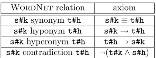
Function extract–local–axioms extracts the local relevant axioms, i.e. the axioms relating concepts within a single structure. The idea is to rephrase the ontological relations between senses into logical relations. Consider again the senses florence#2 and italy#3 associated to the nodes FLORENCE and ITALY in Figure 2.1.b. The ontological knowledge tells us that ‘italy#3 hyperonym florence#2’. This can be expressed by the axiom ‘florence#2→italy#3’. In HC-CtxMatch, local axioms are built by translating WordNet relations into formulas according to Table 3.1.
3.2.2
HC–specific functions for semantic–comparison
The top–level function semantic–comparison calculates the semantic rela-tion between the formulas approximating the meaning of two nodes. In this section we describe the structural dependent functions called by this function: extract–global–axioms and build–deductional–formulas.
extract–global–axioms works exactly as extract–local–axioms. The only difference is that the axioms extracted express relations between concepts belonging to different structures. Consider for example that the two senses tuscany#1 and italy#3 have been associated respectively to nodes TUSCANY and ITALY in Figure 2.1.b. The ontological relation is ‘italy#3 hyperonym tuscany#1’, which can be expressed as ‘tuscany#1 → italy#3’. The rules of translation from WordNet senses to axioms are the same as for the function extract–local–axioms.
WordNet relation axiom s#ksynonym t#h s#k≡ t#h s#khyponym t#h s#k→ t#h s#khyperonym t#h t#h→ s#k s#kcontradiction t#h ¬(t#k ∧ s#h) Table 3.1: WordNet relations and their axioms.
In our approach, the problem of finding the relation between two nodes is encoded into a satisfiability problem. build–deductional–formulas defines the satisfiability problems needed by defining (i) the set R of possible relations holding between concepts and, for each such relation r ∈ R, (ii) the formula which expresses the truth conditions for this relation. Clearly, the set R of possible relations depends on the intended use of the structures we want to map. For HC-CtxMatch we choose the following set–theoretical relations: ≡, ⊆, ⊇, ⊥ (⊥ means that the two concepts are disjoint).
Relation Formula
⊥ (α ∧ β ∧ γ) → ¬(φ → ψ)i ≡ (α ∧ β ∧ γ) → (φ ≡ ψ)i ⊆ (α ∧ β ∧ γ) → (φ → ψ)i ⊇ (α ∧ β ∧ γ) → (ψ → φ)i
Table 3.2: The satisfiability problems for concepts hφ, αi and hψ, βi, with global axioms γ.
Table 3.2 reports the pairs hrelation,formulai representing the satisfiability problems associated to each relation between concepts we consider, given two concepts hφ, αi, hψ, βi, and the formula γ representing the global axioms. The result of this function is simply an array k[] containing these pairs.
Consider the problem of checking whether FLORENCE in the right-hand struc-ture in Figure 2.1.b is, say, equivalent to the node FLORENCE in the left-hand structure. Following are the concepts and axioms extracted by the two struc-tures:
concept 1: image#1 ∧ tuscany#1 ∧ florence#2 (3.1) local axiom 1: florence#2→ tuscany#1 (3.2) concept 2: image#1∧ italy#3 ∧ florence#2 (3.3) local axiom 2: florence#2→ italy#3 (3.4) global axiom: tuscany#1→ italy#3 (3.5) Checking equivalence then amounts to checking the following logical con-sequence 3.2 ∧ 3.4 ∧ 3.5 |= (3.1 ≡ 3.3). By the properties of propositional consequence, we can rephrase it as follows: |= (3.2 ∧ 3.4 ∧ 3.5) → (3.1 ≡ 3.3). It is easy to see that this latter formula is valid. So we can conclude that the relation holding between the two nodes FLORENCE is “equivalence”, which is the intuitive one.
In particular, the function satisfies checks for the validity of a formula. In our implementation a standard SAT–solver is used for this task.
Chapter 4
Improving HC-CtxMatch
4.1
The general approach
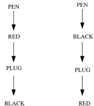
The algorithm HC-CtxMatch, as defined in the Chapter 3, builds a boolean formula approximating the meaning expressed by a node as a conjunction of dis-junctions. Using this kind of encoding leads to a general problem. Consider the very simple structures depicted in Figure 4.1. Imagine to run HC–CtxMatch for finding the relation holding between the two nodes BLACK and RED on the low: it returns the wrong result ‘≡’ (equivalence).
The reason of it is that the formulas approximating the concepts expressed by the two nodes are:
pen#1∧ red#1 ∧ plug#1 ∧ black#1 and
pen#1∧ black#1 ∧ plug#1 ∧ red#1
for BLACK and RED nodes respectively. Because of the commutative property on logical connectives, there is no significant difference between the two formulas. But, how we can simply argue, the relation holding between the two nodes BLACK and RED should have been ‘⊥’ (no relation). In fact the node BLACK of the left structure means intuitively ‘the red pens with the black plugs’ while the node RED of the right structure means intuitively ‘the black pens with the red plugs’, so that the sets of objects described by the two node are distinct (their intersection is the empty set).
In this paper we propose a new approach for improving the encoding process of HC-CtxMatch. The general idea is the following:
1. to use a more expressive and powerful logics, able to handle the semantic richness of structures labelled with natural language;
2. to obtain grammatical and ontological knowledge, helping us to better approximate the meaning expressed by a node;
PEN RED PLUG BLACK PLUG PEN BLACK RED
Figure 4.1: CtxMatch problem
3. to face the problem of building the formula to be associated to a node in two steps: (i) individuating ‘semantic atoms’ present into the structures, and (ii) to combine them to build ‘molecules’.
For a sake of simplicity and because of the fact we want to focus on the process of building formulas, we imagine to use the structure depicted in Fig-ure 4.2, where each node has been pre–processed by the algorithm until to each node is associated exactly one concept (i.e. one sense). To extend the approach to the more general case (when two or more senses are associated to a node) is quite simple: the process we are going to present works indifferently on a set of senses.
4.1.1
Using DL
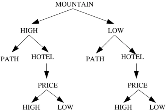
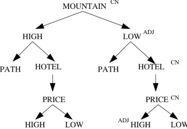
As we said before, the first step is to individuate a more suitable logics than propositional one. For this version of the algorithm we choose Description Log-ics. Consider for example the structure depicted in Figure 4.2. What we want to obtain is such an encoding which allow us to find that the relation holding between the two low central nodes HIGH and LOW is ‘disjoint’.
From an intuitive point of view, we want to say that the node HIGH in the low right means ‘Hotels with high price located in low mountains’, while the node LOWin the low left means ‘Hotels with low price located in high mountains’. In description logics we can approximate these formulas by:
hotelu ∀HasPrice.high u ∀IsLocated .(mountain u ∀HasHeight.low) and
hotelu ∀HasPrice.low u ∀IsLocated .(mountain u ∀HasHigh.high) Such an encoding allow us to say that the two nodes have no relation. In fact, the concepts described by the formulas hotel u ∀HasPrice.high and
HIGH LOW MOUNTAIN HIGH LOW PRICE PRICE HIGH LOW HOTEL HOTEL PATH PATH
Figure 4.2: A more complicated structure
hotelu∀HasPrice.low are mutually exclusive, so far as the concepts mountainu ∀HasHigh.high and mountain u ∀HasHigh.low.
Description Logics is then enough expressive to encode the semantic richness of structures labelled with natural language (we want to manage). In particular, using Description Logics allows us to encode three different types of function-ality a node can assume into a structure: concept, role and value. Consider again the node HIGH in the low right of the structure depicted in Figure 4.2 and the following associated formula:
hotelu ∀HasPrice.high u ∀IsLocated .(mountain u ∀HasHeight.low) We can recognize the following three kinds of functionality associated to different nodes:
concept: for example the nodes HOTEL and MOUNTAIN. They represent the nodes which have the property of attracting nodes with modifier functionalities. In our case, the right low node HIGH refers clearly to the node HOTEL, while the second level node LOW refers clearly to the role PRICE which refers to the node HOTEL. In DL the nodes with this property are translated into concepts: hotel and mountain
role: for example the nodes PRICE. This node represents a role for node HOTEL whose fillers are expressed by nodes HIGH and LOW. In the formula this is encoded into the role HasPrice.
value: for example the nodes MOUNTAIN, LOW, HIGH. Roles can be explicitly expressed by the structure, as in the case of HasPrice (node PRICE), or implicitly expressed, as in the case of IsLocated and HasHeight. The nodes belonging to the functional category ‘value’ represents the filler for explicit and implicit roles. In the formula the three nodes MOUNTAIN, LOW, HIGH
HIGH LOW MOUNTAIN HIGH LOW PRICE PRICE HIGH LOW PATH CN CN CN ADJ ADJ
PATH HOTEL HOTEL
Figure 4.3: A structure enriched with grammatical categories
are translated into the following couple role/filler isLocated .(mountain u ∀hasHeight.low), hasHeight.low and hasPrice.high. Note that MOUNTAIN is both a concept and a filler.
To individuate which functional category a node belongs to, we need at least of two kind of knowledge: grammatical and ontological.
4.1.2
Grammatical knowledge
In this paper we use only two grammatical categories: common nouns (CN) and adjectives (ADJ). We believe we can extend conservatively (and easily) the encoding process for handling some other syntactical categories, as proper names, infinite and past participle verbs, while for other kinds of syntactical categories the analysis could be extremely more complicated.
We imagine, for a sake of simplicity, to have a black box returning the exact syntactical category of some input (an example of input could be a sense associated to a node). Imagine, for example, that we want to determine the syntactical categories of the nodes lying in the path from root to the low right node HIGH. The result of accessing the grammar should be that one depicted in Figure 4.3.
Syntactical information allow us to have a first approximate hypothesis on the functionality to be associated to a node. For example, from the fact that the adjective HIGH is a child of the common noun MOUNTAIN, we can deduce that, most probably, the node HIGH can be interpreted as a filler (value) for some generic role existing between the concepts expressed by the node MOUNTAIN and by the node HIGH.
HIGH LOW MOUNTAIN HIGH LOW PRICE PRICE HIGH LOW HOTEL
PATH PATH HOTEL
RELATION:IsLocated
RELATION:HasHeight
ROLE:HasPrice
FILLER:HasPrice
Figure 4.4: A structure enriched with ontological knowledge
4.1.3
Ontological knowledge
The second kind of knowledge we need is the ontological knowledge. As for grammatical knowledge, we think of ontology as a black box where, given some inputs, it returns the wanted ontological knowledge (if it exists).
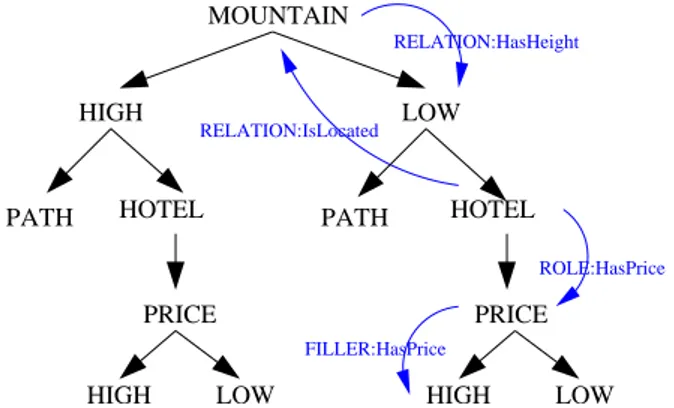
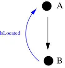
An example of ontological request is the following: imagine we want to know if it exists a relation between the concepts associated to the nodes MOUNTAIN and LOW of Figure 4.4. We inquire ontology–black box given in input the two concepts: the expected result is that exists a role HasHeight tieing ‘mountain’ and ‘low’. Note that the relation is directional, i.e. the role holds between mountain and low (‘mountains have an height that can be low’) but not vice-versa.
More specifically, we need essentially three kinds of informations: • the kind of (implicit) role existing between two nodes;
• the fact that a node can be a role itself;
• the fact that a node can be a filler for some role.
The expected result of accessing ontology for determining these three kinds of relationships holding between the nodes lying on the path from root to the lower right node HIGH of Figure 4.2 should be that one depicted in Figure 4.4. Note that we sign the relations as arrows, because of the directionality of the relationship. If no relation is found, no arrow is associated to the structure.
In particular, we should find four relations:
RELATION:HasHeight : It means that a relation ‘HasHeight’ holds between the nodes MOUNTAIN and LOW, and means exactly that ‘mountains has a low height’;
RELATION:IsLocated : It means that a relation‘IsLocated’ holds between the nodes HOTEL and MOUNTAIN, and means exactly that ‘hotels are located in mountains’;
ROLE:HasPrice : This relation holds between the nodes HOTEL and PRICE, and means exactly that ‘hotels has a price’. Note that the arrow is explic-itly declared as ROLE: in fact, the concept ‘Price’ is not a filler for some role, but it is the role itself.
FILLER:HasPrice : This relation holds between the nodes HIGH and the role HasPrice, and means exactly that ‘high’ can be a filler for the role ‘HasPrice’.
4.2
Building formulas
In this section we describe informally the steps to follow for building a formula approximating the meaning expressed by a node. Note that, as we said in Section 4.1, we consider the grammatical and ontological knowledge as a black box returning the informations we need. For make things simpler, we imagine to have defined four functions:
• function accessing the grammar:
find-syncat(node n) : This function takes as input a node and returns the associated grammatical category;
• functions accessing the ontology:
find-relation(node n, node m) : This function takes as input two nodes and returns the (directional) relationship holding between the nodes n and m if any, N ull otherwise. Note that access-onto-logy(n,m) may be different from access-ontology(m,n); is-role(node n, node m) : This function takes as input two nodes and
returns a role R if n is one of the possible role of m, N ull otherwise; is-filler(node n, role r) : This function takes as input a node n an a role r and returns T RU E if n can be a filler for r, F ALSE otherwise.
4.2.1
Individuating the functionality of a node
This step assume a crucial role. The general idea is to combine grammatical and (some) ontological knowledge1
for individuating the functionality of a node, i.e. if a node should have considered a concept, a value or a role. At this level the process can be considered syntactical : in fact we try simply to individuate the main concepts present in the structure (i.e. nodes with ‘concept’ functionality) and their (eventual) modifiers (i.e. nodes with ‘role’ or ‘value’ functionality).
1
HIGH LOW MOUNTAIN HIGH LOW PRICE PRICE HIGH LOW CN ADJ CN ADJ CN V R V C C
PATH HOTEL PATH HOTEL
FILLER:HasPrice
ROLE:HasPrice
Figure 4.5: A structure enriched with functional categories
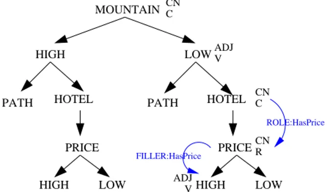
For example, if we consider the Figure 4.2, we intuitively understand that the node MOUNTAIN is a ‘concept’ and that the node LOW is a modifier of the concept ‘mountain’, i.e. is a filler for some (implicit) role. Furthermore we clearly understand that HOTEL is a concept, and that HIGH is the filler of an (explicit) role HasPrice, defined by the node PRICE.
More formally, given a node n, we associate the functional category F C by means of the following recursive rules:
1. s = find-syncat(n)
2. if s = ‘ADJ’, then F C = ‘V’ (value); 3. if s = ‘CN’, then F C = ‘C’ (concept);
4. if s = ‘CN’ and if is-role(n, FATHER(n)) 6= N ull, then F C = ‘R’ (role); 5. if s = ‘CN’ and F C(FATHER(n)) = ‘R’ and
is-filler(n,is-role(FATH-ER(n),FATHER(FATHER(n)))) = TRUE, then F C = ‘V’ (value). The rule 1 simply determines the syntactical category of a node. The rule 2 says that an adjective is always considered as a filler for some role. The idea is that an adjective must refer always to some noun, so it should be always a filler. The rule 3 says that a common noun is considered as a concept. This is a default condition, which can be modified by rules 4 and 5. The rule 4 says that if a node is a common noun but it can be considered a role (with respect to its father node), than the functional category is ‘role’. This is the case of node PRICE in structure of Figure 4.4. It is a common noun, but it can be considered as a role (HasPrice) for the node HOTEL. The rule 5 concludes the process. The idea is that a node with ‘role’ functionality should be followed by a filler: so, (i) if the following node is an adjective, it is intended by default to be the filler (for rule 2), while (ii) if the following node is a common noun, its functionality becomes ‘value’ only if we have the ontological information allowing us to do that. The
HIGH LOW MOUNTAIN HIGH LOW PRICE PRICE HIGH LOW PATH C V R V C
HOTEL PATH HOTEL
Figure 4.6: The semantic atoms
result of applying rules 1–5 to the structure depicted in Figure 4.4 is depicted in Figure 4.5, together with the ontological and grammatical knowledge useful for this process.
4.2.2
Individuating the semantic atoms
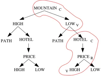
The next step has the task of individuating the semantic atoms lying on a path. A semantic atom can be intuitively defined as the minimal meaningful unit: the idea is that a node with a concept functionality, followed by all the atoms which modifies it, constitutes something we can handle as an unit. In fact, nodes with ‘role’ or ‘value’ functionality assumes meaning only when associated to the main concepts they refer to. Consider for example Figure 4.6. In the path from root to the low right node HIGH, we can individuate two atoms:
1. the atom constituted by nodes MOUNTAIN and LOW, where ‘mountain’ is the main concept modified by ‘low’;
2. the atom constituted by nodes HOTEL, PRICE and HIGH, where ‘hotel’ is the main concept modified by ‘price’ and ‘low’.
More formally, an atom can be defined as a set of nodes constituted exactly by one node with ‘conceptual’ functionality and all the nodes with ‘role’ and ‘value’ functionality modifying the ‘conceptual’ node. A trivial consequence of it is that, considering a path from root to a node n, there will be as many atoms as nodes with ‘conceptual’ functionality lying in the path.
The procedure for exactly individuate the atoms is the following. Let A[] be an empty array of sets of nodes (each set of nodes being an atom) and i an index, set to the value -1. Let n the node whose path (from root) we want to analyze:
1. P = path from root to n 2. for each p ∈ P (a) if FC(p) = ‘C’, then • i = i+1 • p ∈ A[i] (b) if FC(p) = ‘R’, then p ∈ A[i] (c) if FC(p) = ‘V’, then p ∈ A[i]
The process is very simple, and the final result of applying the rules 1–2c to the path from root to the lower right node HIGH is depicted in Figure 4.6, together with the functional category useful for this task.
4.2.3
Building the formula
The final step is to build the formula expressing the meaning of a node n. To do that, we simply handle the atoms present into the path (from root to the node n). In particular, we perform two sub–steps: (i) for each atom, we build a formula expressing its meaning and (ii) we combine this formulas into a unique formula expressing the meaning of the node into the structure.
Imagine we want to build up the meaning associated to the low right node HIGH: we need to build the two formulas approximating the meaning expressed by the atoms depicted in Figure 4.6 and to combine them.
Building the atom formulas
The first step is really simple. In each atom there is only one node with ‘con-ceptual’ functionality and a set of nodes with ‘role’ and ‘value’ functionalities. The ‘conceptual’ node, i.e. the node with the functionality ‘C’, can be trans-lated into Description Logics as a concept, the nodes with functionality ‘V’ as a filler, while the nodes with functionality ‘R’ as roles. The sub-step is reached by means of the following recursive rules:
for each atom A lying in the path: 1. φ = N ull
2. let r the node with functionality ‘C’ (i.e. the main node)
3. associate to r the formula φ = r (i.e. the formula is equivalent to the concept associated to the node);
4. for each following node n ∈ A: (a) R = find-relation(n,r) (b) if R = Null, then R = Rn/r
(c) if F C(n) = ‘V’ and F C(F AT HER(n)) 6= ‘R’, associate to n the formula φ = φ + u∀R.n
(d) if F C(n) = ‘V’ and F C(F AT HER(n)) = ‘R’, associate to n the formula φ = φ + .n
(e) if F C(n) = ‘R’, then R = is-role(n,r). Associate to n the formula φ = φ + u∀R
The procedure starts by individuating the main concept and translating it into a DL concept. Then, it finds the role holding between two nodes of the atom and, for each combination of functional category, it builds the DL modifiers. In particular note the steps 4(a–b): in this procedure we access ontology by means of the function find-relation() for finding the relation holding between the main node and some modifier. If no relation is founded, we define a generic relation Rn/r. For example, if no relation holding between the nodes MOUNTAIN
and LOW was founded, the following formula would have been built: mountainu ∀Rmountain/low.low
expressing the fact that ‘low’ is a filler of a generic role existing between ‘mountain’ and ‘low’. This rule allow us to built the formula in any case.
Applying this procedure to the path from root to the low right node HIGH, we obtain the two formulas:
mountainu ∀HasHeight.low and
hotelu ∀hasPrice.high
respectively for the upper and the lower atoms depicted in Figure 4.6. Combining atoms
After having built the formulas associated to the semantic atoms, we try to com-bine these formulas (to build a molecule!), taking into account the relationships holding between atoms, namely relationships holding between the main nodes (the nodes of functional category ‘C’) of the atoms composing the molecule. In our example, we find that there is an IsLocated role holding between HOTEL and MOUNTAINS, in the sense that ‘hotels are located in mountains’. General situation is depicted in Figure 4.7. The fact that exists a relation between the two atoms allows us to say that one of the two atoms can be considered as a modifier of the other one, and translated into a role in Description Logics. The final result of applying these rules should be the following:
A
B
IsLocated
Figure 4.7: Combining atoms
Abstracting from our example, the general rules for combining atoms are the following. Let n be the node we want to build up the associated formula, and let A be the set of atoms lying in the path from root to n. Furthermore, let f (A) be the formula associated to the atom A by the previous step. Then:
1. R = the first atom in A 2. formula φ = f(R)
3. for each remaining atom A ∈ A, accessing top down: (a) a = main node in A
(b) for each ancestor B of A • b = main node in B • R = find-relation(a,b) • Ri = find-relation(b,a)
• choose R or Ri
(c) if R = IsA or R = P artOf , then φ = φ[b/(f (A))] (d) if Ri = IsA or Ri = P artOf , then φ = φ[a/(f (B))]
(e) if R 6= N ull, then φ = φ[f (B)/f (A) u ∀R.(f (B))] (f) if Ri6= N ull, then φ = φ[f (B)/f (B) u ∀Ri.(f (A))]
The idea expressed by this algorithm is simple. If we find some relation between an atom A and some ancestor B, A becomes a modifier for B, while if we find a relation between B and A, B becomes a modifier for A. The result of applying this final step to the atoms depicted in Figure 4.6 is the following formula:
hotelu ∀hasPrice.high u ∀isLocated .(mountain u ∀hasHigh.low) which is exactly that one we want.
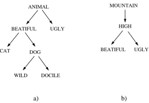
Note that we use two special rules for IsA and P artOf relations: imagine a situation as depicted in Figure 4.8.a, where we are in presence of a IsA relation.
BEATIFUL UGLY DOG DOCILE WILD HIGH UGLY BEATIFUL a) b) ANIMAL CAT MOUNTAIN
Figure 4.8: Two different structures
Imagine you want to build up the formula approximating the meaning associated to node WILD.
The algorithm builds the right formula
DOGSu ∀HasBehaviour .WILD u ∀HasBeauty.BEATIFUL
In particular, the algorithm substitutes the concept ‘animal’ with the concept ‘dog’, because it is a redundant information. In fact, the function build-ctx-meaning (see algorithm 3.2) extracts from the ontology the local axiom (see chapter 3) DOG w AN IM AL.
Another situation well-handled by this algorithm is that one depicted in Figure 4.8.b, where we have a chain of adjectives. The formula associated to the node BEAUTIFUL is the followed
MOUNTAINSu ∀HasHeight.HIGH u ∀HasBeauty.BEATIFUL which is the right one.
4.3
Handling the ambiguity
The step we describe in section 4.2.3 has a strong assumptions concerning the process of discovering relationships between atoms: it hypothesizes to find ex-actly one relation holding between two atoms.
The general idea is that we are in a perfectly not-ambiguous situation. Of course this is not the more general and frequent case. The kinds of ambiguity we can encounter are four:
1. no relation is founded between two atoms;
2. two or more relations are founded between two atoms;
3. a relation between A and B and a relation between B and A is founded (reciprocal relationships);
4. an atom has relations with more than one ancestor and/or siblings. The ambiguous situation 1 is mutually exclusive with the situations 2-4, while situations 2-4 can be present at the same time. In the next section we propose a general approach to handle this kinds of ambiguity.
4.3.1
No relation between two atoms
A
B
C
IsLocated
Figure 4.9: No relation between two atoms
Consider the Figure 4.9. In this case, we are in presence of three atoms (A, B, C), but we find a relation only between A and B. No relation has been founded between C and some other atom. In this case we should build two different formulas. In fact, if it’s simple to understand that if the relation between the first two atoms has no ambiguity, and can be solved as
Au ∀IsLocated .B
the same cannot be done for the third atom (C). Essentially, there can be two possible interpretations:
Cu ∀R.(A u ∀IsLocated .B) or
(A u ∀IsLocated .B) u ∀R.C
Handling the ambiguity in this way leads to a blow up in the number of formulas: in the worst case, hand Lind n atoms means to have 2n possible
interpretations. To make things easier, we choose to handle the ambiguity in a more simple way, i.e. to use the intersection builder (u) of Description Logics. This means that for building the formula associated to the atom C, instead of to have the two formulas described before, we have the unique formula:
which intuitively means the intersection between the concept A (as modified by the role IsLocated ) and the concept C. From a formal point of view, we need to insert the following rule in the algorithm described in section 4.2.3:
if R = N ull and Ri= N ull, then φ = (φ) u f (A)
4.3.2
Multiple relations between two atoms
Concerning the ambiguity caused by the presence of more than one relation, we need to distinguish between two cases:
sense#1 sense#2 sense#3 B sense#4 A IsLocated HasPart
Figure 4.10: Multiple relations between two atoms referring to different senses
• the ambiguity regards two or more different senses associated to the main node of the atoms;
• the ambiguity regards an unique sense.
In the first case the ambiguity concerns the senses associated to the main nodes of the atoms, so it can be treated as a disjunction. Consider the ex-ample of Figure 4.10. The two relations founded, respectively IsLocated and HasPart, refer to different senses, so that the following relations hold: sense#3 ∀IsLocated .sense#1 and sense#4 ∀HasPart.sense#2.
The interpretation of the atom B is so:
(sense#3 u ∀IsLocated .sense#1) t (sense#4 u ∀HasPart.sense#2) This means simply that for this atoms we have two possible interpretations: because of the lack of ontological information we are not able to discard one of these ones. The case where the multiple relations refers to the same sense is more interesting, because of the presence of a real ambiguity on relations.
Consider the general case depicted in Figure 4.11, where the ambiguity re-gards a single sense associated to a node into the atom. In this case we are in presence of two ore more relations holding between an atom A and another atom B.
This kind of ambiguity can be managed building a formula as follow: Bu (∀IsLocated .A t ∀HasPart.A)
B A
IsLocated HasPart
Figure 4.11: Multiple relations between two atoms
4.3.3
Bidirectional relations
In presence of bidirectional relations between atoms, the ambiguity can not be maintained at the modifiers level.
A
B
IsLocated HasPart
Figure 4.12: Bidirectional relations
There are two possible interpretations: B u ∀IsLocated .A or A u ∀HasPart.B. Because of the fact that we are not able to solve this ambiguity, we need to associate the following formula
(B u ∀IsLocated .A) t (A u ∀HasPart.B) both to atom A and B.
4.3.4
Multiple relations with ancestors or siblings
The only case of real ambiguity in presence of multiple relations with ancestors or siblings is that one depicted in Figure 4.13, where a single atom is a modifier of two different atoms.
There are two possible interpretations. If we consider the relation IsLocated we obtain the formula:
(B u ∀IsLocated .A) u C
while if we consider the relation HasPart we obtain the formula: (C u ∀HasPart.A) u B
B A
C IsLocated
HasPart
Figure 4.13: Multiple relations with descendants
If we take a disjunction between this two formulas, we obtain the following one:
((B u ∀IsLocated .A) u C) t ((C u ∀HasPart.A) u B)
4.4
Catalogues – Cat-CtxMatch
This approach has the further advantage to be easily generalized to catalogues. In fact, the clustering into the three functional categories ‘C’ (concept), ‘R’ (role) ad ‘V’ (value) is explicitly present into a catalogue. Consider the catalogue depicted in Figure 4.14, which represents the same structure of the Figure 4.2.
MOUNTAIN HasHeight=Low,High
HOTEL HasPrice=Low,High PATH
Figure 4.14: A simple catalogue
As we can easily see, the problems of determining the functionality category of each element of the structure and of building the semantics atoms is solved a priori. The only problems remained are (i) to find eventual relations between atoms and (ii) to provide to combine the atoms in order to obtain the formula to be associated to each node. For this task, the procedure to be followed is the same we described.
Appendix A
The algorithm
In this appendix we briefly define the pseudo–code for the algorithm. In partic-ular, this version of the pseudo–code is able to manage the ambiguity regarding the absence of relations between atoms, but not the other kinds of ambiguities.
In the algorithm A.1 is described the pseudo–code substituting the function individual-concept (see algorithm 3.5).
Algorithm A.1 new-individual–concept(t, SynS, T, O)
.label t
.sense SynS[][]
.structure T
.ontology O
VarDeclarations
relation R = N ull, Rel = N ull formula η = N ull
path P Conc[]
.Array of individual concepts expressed by a node
FunCat[]
.Array of functional categories associated to nodes
Atoms[]
.Array of sets of nodes (each set is an atom)
1 for each SynS[t][i] in SynS[t][] do
2 foreach sibling y of t in T do
3 for each SynS[y][k] in SynS[y][] do
4 R ← access–ontology(SynS[t][i], SynS[y][k], O);
5 if R= ‘hyperonymy’ then Rel ← ‘hyperonymy’;
6 if (rel 6= N ull) then replace SynS[t][i] in SynS[t][] with ‘SynS[t][i] ∧
¬SynS[y][k]’;
7 P ← path from root to t in T ;
.Path from root to node t
8 for each p ∈ P
9 Conc[p] ←W
sense∈pSynS[p][i];
.To each node is associated a disjunction of senses
10 FunCat[] ← associate-fun-cat(P, Conc[]); 11 Atoms[] ← build-semantic-atoms(P,FunCat[]);
12 AtomFormulas[] ← build-semantic-atom-formula(Atoms[],FunCat[],Conc[]); 13 η ← combining-semantics-units(Atoms[], AtomFormulas[], Conc[]);
In the following, we proceed to define in detail the new four functions called by lines 10–13 of algorithm A.1. The first one, the associate-fun-cat function, has the main goal to associate the functional category to each node.
Algorithm A.2 associate-fun-cat(P, Conc[])
.path P
.array of individual concept Conc[]
VarDeclarations syntactical category s; path P
FunCat[]
.Array of functional categories associated to nodes
1 for each node p ∈ P accessing top–down
2 c ← Conc[p]
3 s ← find-syncat(c);
4 ifs = ‘ADJ’, then FunCat[p] ← ‘V’;
5 ifs = ‘CN’, then FunCat[p] ← ‘C’;
6 ifs = ‘CN’ and if is-role(c,FATHER(c)) 6= ‘Null’, then FunCat[p] ← ‘R’;
7 ifs = ‘CN’ and FunCat[FATHER(p)] = ‘R’ and
is-filler(c,is-role(FATHER(c),FATHER(FATHER(c)))) = ‘TRUE’,
thenFunCat[p] = ‘V’;
.These steps associates to each node one of the three possible functional categories: ‘V’ (value or filler), ‘C’ (concept) or ‘R’ (role)
The second function, build-semantic-atoms, tries to determine the se-mantic atoms present in some path.
Algorithm A.3 build-semantic-atoms(P, FunCat[])
.path P
.array of functional categories FunCat[]
VarDeclarations array Atoms[];
.Array of sets of nodes. Each set is an atom
index i;
1 for each p ∈ P accessing top–down
2 ifFunCat[p] = ‘C’, then
3 i ← i + 1;
4 p ∈ Atoms[i];
5 ifFunCat[p] = ‘V’, then p ∈ Atoms[i];
6 ifFunCat[p] = ‘R’, then p ∈ Atoms[i];
The third function, semantic-atom-formulas, has the aim of build-ing the formulas associated to each atom. The task is quite simple, because we handle only one concept and its modifiers.
Algorithm A.4 build-semantic-atom-formulas (Atoms[], FunCat[], Conc[])
.array of atoms Atoms[]
.array of functional categories FunCat[]
.array of individual concepts Conc[]
VarDeclarations formula φ;
array AtomFormulas[];
1 for each Atoms[i]
2 φ= N ull;
3 r = node n ∈ Atoms[i] s.t. FunCat[n] = ‘C’
.The node is unique and it is the always the first one
4 φ← Conc[p]
.the formula is equivalent to the concept associated to the node
5 foreach following node p ∈ Atoms[i]
6 R = find-relation(r,p)
7 if R = Null, then R ← Rn/r;
8 if F C(p) = ‘V’ and F C(F AT HER(p)) 6= ‘R’, φ ← φ + u∀R.Conc[p]
9 if F C(p) = ‘V’ and F C(F AT HER(n)) = ‘R’, φ ← φ + .Conc[p]
10 if F C(p) = ‘R’, then R = is-role(p,r) and φ ← φ + u∀R
11 AtomFormulas[i] ← φ
The last function combining-semantic-atoms has the main task of com-bining atoms to form molecules.
Algorithm A.5 combining-semantic-atoms(Atoms[], AtomFormu-las[], Conc[])
.array of atoms Atoms[]
.array of formulas AtomFormulas[]
VarDeclarations formula φ
1 R ← Atom[0]
.R is the first atom accessing top–down
2 φ= AtomFormulas[R];
3 for each atom Atoms[i¿0] accessing top down
4 a = node n ∈ Atoms[i] s.t. FunCat[n] = ‘C’;
5 foreach ancestor Atoms[j] of Atoms[i]
6 b = node n ∈ Atoms[j] s.t. FunCat[n] = ‘C’
7 R ← find-relation(a,b);
8 Ri← find-relation(b,a);
9 choose R or Ri;
10 if R = N ull and Ri= N ull then φ ← φ + u (AtomFormulas[A])
11 ifR = IsA or R = P artOf then φ ← φ(Conc[b] / (AtomFormulas[A]))
.The formula is the same as the father formula except that the concept expressed by node b is substituted by the formula associated to atom A
12 if Ri= IsA or Ri= P artOf , then φ ← φ(Conc[a]/(AtomFormulas[B]))
13 if R 6= N ull, then φ ← φ(AtomFormulas[B]/AtomFormulas[B] u∀ R.
(Atom-Formulas[A]))
14 if Ri 6= N ull, then φ ← φ(AtomFormulas[A]/AtomFormulas[A] u∀ R.
(AtomFormulas[B])) 15 Return η;
Bibliography
[1] M. Bonifacio, P. Bouquet, and P. Traverso. Enabling distributed knowl-edge management. managerial and technological implications. Novatica and Informatik/Informatique, III(1), 2002.
[2] P. Bouquet, editor. AAAI-02 Workshop on Meaning Negotiation, Edmonton, Canada, July 2002. American Association for Artificial Intelligence (AAAI), AAAI Press.
[3] G. Cerchia. Logica e linguistica. il contributo di montague. Laterza, 1992. [4] Christiane Fellbaum, editor. WordNet: An Electronic Lexical Database. The
MIT Press, Cambridge, US, 1998.
[5] P. Bouquet B. Magnini, L. Serafini, and S. Zanobini. A SAT–based algo-rithm for context matching. In P. Blackburne, C. Ghidini, R.M. Turner, and F. Giunchiglia, editors, Proceedings of the 4th International and Inter-disciplinary COnference on Modeling and Using Context (CONTEXT-03). Stanford University (CA), June 23-25, 2003, volume 2680 of Lecture Notes in Artificial Intelligence. Springer Verlag, 2003.
[6] R. Montague. On the nature of certain philosophical entities. 1960. [7] R. Montague. Contemporary philosophy: A survey. 1968.
[8] R. Montague. English as a formal language. 1970.
[9] P. Bouquet L. Serafini and S. Zanobini. Semantic coordination: a new ap-proach and an application. In Proceedings of the 2nd International Semantic Web Conference (ISWO’03). Sundial Resort, Sanibel Islands, Florida, USA, October 20-23, 2003, 2003.