Fluctuating hydrodynamics model for homogeneous and heterogeneous vapor bubble nucleation

Dipartimento di Ingegneria Meccanica e Aerospaziale

Dottorato di Ricerca in Meccanica Teorica e Applicata XXXI Ciclo

Fluctuating Hydrodynamics

Model for Homogeneous and

Heterogeneous Vapor Bubble

Nucleation

PhD Candidate Mirko Gallo

Supervisor

Prof. Carlo Massimo Casciola Tutor

Fluctuating Hydrodynamics Model

for Homogeneous and

Heterogeneous Vapor Bubble

Nucleation

Mirko Gallo

2 aprile 2019

Man is a mystery. It needs to be unravelled, and if you spend your whole life unravelling it, don’t say that you’ve wasted time. I am studying that mystery because I want to be a human being.

Abstract

At the molecular scale, even in conditions of thermodynamic equilibrium, the fluids do not exhibit a deterministic behavior. Going down below the micrometer scale, the effects of thermal fluctuations play a dominant role in the dynamics of the system, calling for a suitable description of thermal fluc-tuations. These models not only play an important role in physics of fluids, but a deep understanding of these phenomena is necessary for the progress of some of the latest nanotechnology. For instance the modeling of thermal fluctuations is crucial in the design of flow micro-devices, in the study of bio-logical systems, such as lipid membranes, in the theory of Brownian engines and in the development of artificial molecular motor prototypes. Another problem with a huge technological impact is the phenomenon of nucleation – the precursor of the phase transition in metastable systems – in this context related to bubble formation in liquid-vapor phase transition. Vapor bubbles form in liquids by two main mechanisms: boiling, by increasing the tempe-rature over the boiling threshold, and cavitation, by reducing the pressure below the vapor pressure threshold. The liquid can be held in these metasta-ble states (overheating and tensile conditions, respectively) for a long time without forming bubbles. Bubble nucleation is indeed an activated process, requiring a significant amount of energy to overcome the free energy barrier

and bring the liquid from the metastable conditions to the thermodynami-cally stable state where vapor is observed. Depending on the thermodynamic conditions, the nucleation time may be exceedingly long, the so-called "rare-event" issue. Nowadays molecular dynamics is the unique tool to investigate such thermally activated processes. However, its computational cost limits its application to small systems (less than few tenth of nanometers) and to very short times, preventing the study of hydrodynamic interactions. The latter effects are crucial to understand the cavitation phenomenon in its en-tirety, starting from the vapor embryos nucleation up to the macroscopic motion.

In this thesis a continuum diffuse interface model of the two-phase fluid has been embedded with thermal fluctuations in the context of the so-called Fluctuating Hydrodynamics (FH) and has been exploited to address cavita-tion. This model provides a set of partial stochastic differential equations, whose deterministic part is represented by the capillary Navier-Stokes equa-tions and reproducing the Einstein-Boltzmann probability distribution for the macroscopic fields. This mesoscale approach enables the description of the liquid-vapor transition in extended systems and the evaluation of bub-ble nucleation rates in different metastabub-ble conditions by means of numerical simulations. Such model is expected to have a huge impact on the under-standing of the nucleation dynamics since, by reducing the computational cost by orders of magnitude, it allows the unique possibility of investiga-ting systems of realistic dimensions on macroscopic time scales. In addition, after the nucleating phase, the deterministic equations have been used to address the collapse of a cavitation nanobubble near a solid boundary, sho-wing an unprecedented description of interfacial flows that naturally takes

into account topology modification and phase changes (both vapor/liquid and vapor/supercritical fluid transformations).

Overview

Nucleation is a complex and intrinsically multiscale problem representing the precursor of phase change in first order phase transitions. Among the huge variety of nucleation problems in nature, this thesis is devoted to the study of liquid-vapor phase change inception. The proposed model is based on a mesoscale approach exploiting a diffuse interface approach embedded with thermal fluctuations. The approach I follow in this PhD project is theore-tical and numerical, and basically, can be structured as follows: I coupled a diffuse interface model with fluctuating hydrodynamics, exploiting the model to address homogeneous and heterogeneous nucleation. In order to perform in silico experiments, an in-house parallel code has been developed. Nu-cleation rates, have been calculated by numerically integrated the resulting equations (Landau-Lifshitz-Navier-Stokes equations with capillarity) showing very good agreement with MD simulations as well as more classical approach. The model is also able to capture long terms dynamics in nucleation –not easily detectable with conventional techniques– revealing some interesting effects. In fact, in closed system, the hydrodynamic effects have a great in-fluence on the nucleation dynamics, where the "bubble crowding" strongly change the nucleation rate. Furthermore, I proposed a spherical version of the LLNS, particularly useful when dealing with homogeneous nucleation,

since it is reasonable to assume the spherical shape of nucleation embryos. In addition LLNS equations can be also used in a pure deterministic set-ting, showing a very accurate description of the hydrodynamics of a two phase system. In particular, the model is exploited to study the collapse of a cavitation nanobubble near a solid surface, showing an accurate reproduc-tion of the main physical phenomena detected in the experiments, namely: strong peaks of pressure and temperature, shockwave emission and liquid jet formation.

In the first chapter, an introduction to vapor bubble nucleation will be given, with particular emphasis on cavitation. The main features of the phenomenon are exposed as well as the technological implications. Further-more a brief overview on the state of art and about the importance of using mesoscale approaches in this context will be illustrated.

The second chapter retraces a detailed description of the Van der Walls diffuse interface approach. In the first sections the thermodynamics of a non-homogeneous system is recalled, deriving a thermodynamically consistent equations of motion for a multiphase system. In this context, I proposed a general expression to uniquely identify the solid-fluid contact angle, relating the solid-fluid free energy contributions with the bulk properties of the fluid. Furthermore a rare event technique (String Method) is coupled with the phase field description to address the bubble nucleation rate.

The third chapter recalls the Einstein theory of hydrodynamic fluctua-tions, focusing on capillary fluids. Starting from the probability density functional, under the hypothesis of small fluctuations, the field correlations of a Van der Walls fluid are obtained in a closed form. The celebrated fluc-tuation dissipation theorem is than derived in a phase field context, leading

to the Landau-Lifshitz-Navier-Stokes (LLNS) equations for a capillary fluid. These equations are used to address the vapor bubble nucleation in a meta-stable liquid. Furthermore, I derived a new set of stochastic equations for nucleation, arising from a spherical version of LLNS.

The fourth chapter is focused on the numerical analysis of the LLNS equations, highlighting the principal numerical issues in capillary and sto-chastic equations. The first sections concern the numerical analysis of the deterministic part of the equations, while the other ones are focused on the stochastic part.

Chapter 5 is devoted to draw the conclusions about this research activity, its implications and further possible developments.

The remaining chapters report the papers I published on high-impact peer-review journals. In particular in Chapter 6 the Van der Waals diffuse interface model is exploited to address the dynamics of a cavitation nanobub-ble near solid boundary, and in Chapter 7 the same diffuse interface model is coupled with a fluctuating hydrodynamic theory to study the vapor bub-ble homogeneous nucleation. Chapter 8 report the model extension to study heterogeneous nucleation (paper in preparation).

Finally, since the present PhD project is framed in an interdisciplina-ry context between engineering and physics, in the appendices are retraced the main features of mathematical techniques that are commonly known in the statistical physics community and not entirely taken for granted in the engineering one.

During my PhD work an international collaboration with Dr. X. Noblin from the “Institut de Physique de Nice”lead to the publication of paper con-cerning the acoustics of a micro-confined cavitation bubble [127]. In addition

I was Co-Advisor of three master thesis:

• Forward Flux Sampling technique in Fluctuating Hydrodynamics con-text to study vapor bubble nucleation. Vincenzo Andrea Montagna, master thesis in Nanotechnology Engineering Sapienza University of Rome.

• A numerical Model to address the dynamics of macroscopic bubbles near solid walls. Dario Abbondanza, master thesis in Mechanical En-gineering Sapienza University of Rome.

• Stochastic Models for Bubble Nucleation, Davide Cocco master thesis in Nanotechnology Engineering Sapienza University of Rome.

Published Papers

• Magaletti, F., Gallo, M., Marino, L., & Casciola, C. M. (2015). Dy-namics of a vapor nanobubble collapsing near a solid boundary. In Journal of Physics: Conference Series.

• Magaletti, F., Gallo, M., Marino, L., & Casciola, C. M. (2016). Shock-induced collapse of a vapor nanobubble near solid boundaries. Inter-national Journal of Multiphase Flow.

• Gallo, M., Magaletti, F ., & Casciola, C. M. Fluctuating hydrodynamics as a tool to investigate nucleation of cavitation bubbles.Multiphase Flow: Theory and Applications, 347. 2018.

• Gallo, M., Magaletti, F ., & Casciola, C. M. Thermally activated va-por bubble nucleation: the Landau–Lifshitz/Van der Waals approch. Physical Review Fluids, 2018.

• Scognamiglio, C., Magaletti, F., Izmaylov, Y., Gallo, M., Casciola, C. M., Noblin, X. (2018). The detailed acoustic signature of a micro-confined cavitation bubble. Soft matter.

Papers in preparation

• Gallo, M., Magaletti, F ., & Casciola, C. M. A mesoscale model for Heterogeneous Nucleation.

• Magaletti, F .,Gallo, M., & Casciola, C. M. Coupling a rare event tech-nique with diffuse interface approach for vapor bubble heterogeneous nucleation.

Conferences and workshops

• Hydrodynamic Fluctuations in Soft-Matter Simulations, February 2016 - Prato, Italy (Poster).

• MolSimEng, September 2016 - Milan, Italy (Poster). • Multiphase Flow, June 2017 - Tallin, Estonia (Talk).

• Numerical Simulations of Flow with Particles, Bubbles and Droplets, May 2018 - Venice, Italy (Talk).

• European Fluid Mechanics Conference, EFMC12, September 2018 -Vienna, Austria (Talk).

Indice

Abstract 1

Overview 5

1 Introduction 15

1.1 Nucleation Overview . . . 16

1.2 Metastability and Phase Transitions. . . 19

1.3 Classical Nucleation theory. . . 24

1.3.1 The Blander and Katz Nucleation Rates . . . 27

1.3.2 The Kramers theory . . . 27

1.4 Thermal Fluctuations at Continuum Level . . . 31

1.5 Beyond Classical Nucleation Theory. . . 34

2 Diffuse interface models 37 2.1 Thermodynamic of non-homogeneous systems . . . 38

2.2 The Van der Waals approach. . . 40

2.3 Solid-Fluid Free Energy . . . 44

2.4 The String Method . . . 48

3 Fluctuating Hydrodynamics 59

3.1 Equilibrium Thermal Fluctuations. . . 60

3.1.1 Static structure factor . . . 67

3.2 Fluctuation dissipation balance . . . 67

3.2.1 Restating the LLNS equations with capillarity in terms of entropy functional . . . 72

3.2.2 FDB for the 3D system . . . 73

3.3 FDB for wall bounded systems. . . 77

3.4 Spherical Formulation of Fluctuating Hydrodynamics Equa-tions and its application to nucleation process . . . 80

4 Numerical Analysis of the LLNS Equations with capillarity 91

4.1 The deterministic equations . . . 91

4.1.1 The different mathematical features of the equations . 92

4.1.2 Operator splitting strategy . . . 94

4.2 The stochastic equations . . . 98

4.2.1 Thermal fluctuations for a capillary fluid at equilibrium in a discrete system . . . 99

4.2.2 Discrete static structure factor and weak convergence analysis . . . 102

4.2.3 Static Probability Distributions . . . 104

5 Conclusion and Perspectives 107

Acknowledgments 111

6 Shock-induced collapse of a vapor nanobubble near solid

boun-daries 113

7 Thermally activated vapor bubble nucleation:

the Landau–Lifshitz/Van der Waals approach 155

8 A Mesoscale Model for Heterogeneous Nucleation 181

Appendices 204

A Gaussian Path Integrals 207

B Ito Stochastic Integration 211

C Backward-Forward Kolmogorov Equations 217

D Bubble Kinematics 221

Capitolo 1

Introduction

The fundamental aspect underlying the phase change inception draws simila-rities in a very large number of applications such as vapor bubble cavitation on propeller blades and on turbines, ice formation on aircrafts, drying or de-foaming procedures in the food industry, solidification in material science and alloy production. The variety of technological applications combined with the complex nature of the phenomenon make nucleation a stimulant research area. The main challenging aspect concerning nucleation is its mul-tiscale nature, ranging from the molecular scale up to the hydrodynamic one. From an experimental point of view, quantitative measurements during the phase change inception are not easy to perform, due to the wide spectrum of space-time scales to be investigated. This issue represents also a great challenge for theoreticians who need to develop consistent multiscale models to correctly capture the critical features of the nucleation phenomenon.

This Chapter is devoted to the presentation of the peculiar aspects of nucleation, with particular attention to the nucleation of vapor bubbles in liquids. The main features of the liquid vapor phase transition will be highlighted, as well as the possible technological implications.

1.1 The impact of nucleation phenomena in

na-ture and technological applications

Nucleation is the “incipit” in the formation of a new thermodynamic pha-se, representing the precursor of phase transformation. In particular, the liquid-vapor phase transition can be achieved by two different mechanism: by increasing the temperature up to the boiling threshold, or by decreasing the pressure below the vapor pressure. We will refer to these two processes as boiling and cavitation, respectively. The qualitative mechanism during cavitation of water flowing at ambient conditions, for example, is simple: vapor nuclei locally appear where the liquid accelerates and its pressure de-creases. Inside these bubbles the pressure is as low as the vapor pressure (that at ambient temperature is about 2.3kP a) hence they can survive, and even grow, as long as they remain in the liquid low pressure regions. Howe-ver, when the flow transports them in a region with higher pressure, they suddenly become unstable and collapse. Vapor bubble implosion is a very complicated physical phenomenon, which comprises large bubble deforma-tion and topological changes, shockwave emission and propagadeforma-tion through the liquid, phase transition to and from supercritical conditions [60], and in-tense pressure and temperature peaks on the order of dozens GP a and 104_K,

respectively, [111]. The aforementioned effects are considered the main cause of damage that is observed on the ship propellers, hydraulic turbines, diesel engines [17,14, 120].

Nowadays cavitation is also exploited as a positive source of damage in different areas of applied sciences, for instance in medicine SWL (shock wa-ve lithotripsy) it is used to comminute kidney and gall stones with acoustic

waves and HIFU (high intensity focused ultrasound) for tumor treatment and other surgical applications [27, 29, 70]. In biochemistry applications the vorticity induced during the last stage of bubble collapse is being used to enhance mixing [89], furthermore manipulation of cavitation nuclei is em-ployed in drugs and genetic material delivery, e.g., to enhance biological barrier layer permeability [38,114] . Concerning nuclei manipulation, liposo-mes and microbubbles are designed with a variety of contents, structures and appendage in order to carry drugs to the target site. Drug can be incorpora-ted by themselves, or if insoluble in water, within the lipid layer. After the bubbles/liposomes have reached the specific site, cavitation can be triggered by using ultrasound or laser-pulses. Hence by controlling liquid-jet formation or shockwave emission cell membrane poration (the so-called sonoporation) can be achieved. Recently gene-loaded structures have been used for DNA injection without destroying effects on the cell[19]. In a completely different context cavitation devices have been developed for the treatment of water pollution [1]. In wastewater treatment, the combined mechanical, thermal and chemical effects of bubble collapse are exploited. In particular the pro-duction of free radicals [134] is found to enhance enhances the oxidation of contaminants in water.

Another example of the cavitation occurrence is the phenomenon of crac-king knuckles which have been recently theorized to derive from cavitation bubbles formed into synovial liquid within articulations. According to some authors osteoarthritis can be caused by repeated cavitation events occurring into joints when they are subjected to traction stress [140].

The crucial issue, and the important challenge, is to obtain quantitative information on all the different aspects involved in cavitation. An

appropria-te investigation down to the smallest length and time scale is needed in order to capture all the macroscopic effects. From an experimental point of view, quantitative measurements of relevant physical observables in cavitation are not easy to perform, due to the reduced space-time scales on which the phe-nomenon occurs (ns/µs in terms of time and nm/µm in terms of space), thus developing theoretical and numerical models is crucial in order to achieve a quantitative understanding of cavitation. On the other hand developing a fully consistent theory is still a great challenge for theoreticians. Concerning the bubble dynamics, the first mathematical model was developed by Lord Rayleigh in 1917 and subsequently improved by M. Plesset [118]. Raylei-gh studied the dynamics of a bubble in an incompressible liquid under the assumption of spherical symmetry. He modeled the bubble interface as a ma-thematical, zero-thickness discontinuity, obtaining an evolution equation for the bubble radius. This model has proven to be very useful for predicting the time evolution of the gas pressure inside the bubble, the bubble oscillations, and an overview of the approximate dynamics of the collapse. However the model is not able to predict many other phenomena that characterise cavi-tation: starting from the nucleation phase up to the reabsorption. The main limitations of these sharp interface models emerge when the diffused nature of the vapour-liquid interface becomes important. This typically happens when the size of the bubble is comparable with the vapor-liquid interface thickness, like e.g. in the case of nanobubbles during nucleation inception, and during the last stages of bubble collapse. More complete models are required in these cases to correctly follow the dynamics down to the smallest relevant scales. One possible solution is relaxing the assumption of sharp interface, by adopting, e.g., a phase field approach, to be discussed in full

detail in Chapter 2.

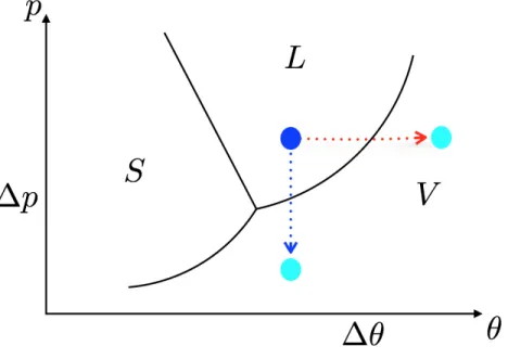
Figura 1.1: The sketch qualitatively describes the state of matter as a function of pressure and temperature. The S-zone represent the solid state, the L-zone the liquid one and the V-zone the vapor phase.

1.2 Metastability and Phase Transitions

Let us now focus on the thermodynamic aspects of the liquid-vapour phase transition analysing the phase diagram in Fig.1.1. Starting from the liquid state, evaporation and cavitation are represented by the red and the blue paths, respectively. This description is however oversimplified and a much more rigorous analysis of these processes is needed for a complete under-standing of the phase transition in liquids [41]. In fact, after reaching the boiling temperature or the vapour pressure, the liquid can remain trapped near coexistence line for a long time (depending on the level of overheating

or stretching). The reason is that bubble nucleation is an activated process that needs to surmount the free energy barrier separating the liquid and the vapor states. As a consequence the system can remain trapped in a me-tastable state, unless the barrier vanishes altogether, i.e. the system is at the so-called spinodal conditions where the transition does not require an activation energy (spinodal decomposition).

Figura 1.2: The sketch qualitatively describes the energetic configurations of a thermodynamic system as a function of a generic reaction coordinate X. The states 1, 2, 3 represent the metastable, the critical and the stable configurations respectively.

In order to better explain this important point, it is worth focusing on a one dimensional system, whose free energy ⌦ is sketched in Fig. 1.2 as a function of a reaction coordinate X. The state X1 is a metastable state,

minimum of the free energy landscape. This “peculiar” state is not the thermodynamic equilibrium state that the system is expected to reach on the long time scale which corresponds to the absolute free energy minimum, X3. Nevertheless, the system could remain trapped for a very long time

around X1. In fact, an amount of energy greater than ⌦⇤ = ⌦2 ⌦1,

with ⌦2 the energy value of the transition state X2, is needed to bring the

system to thermodynamic equilibrium. In thermally activated process the energy is provided by thermal fluctuations. In this case the life time ⌧ of the metastable state is related to the energy barrier as ⌧ / exp( ⌦⇤_/k

B✓),

suggesting the definition of metastability as a stability limited over time. There are many metastable systems in nature. One of the most popular is carbon in the diamond phase at ambient conditions that could undergo, in principle, the diamond-graphite phase transition. In standard conditions, the stable form of carbon is graphite. However the life time of diamond is so long that diamond can remain stable for million years [137,7]. Metastability could be observed also in supercooled water [106,103], (e.g freezing rain, icing aircraft) or in emulsions and colloids [85, 48], and in mechanical systems, for instance when dealing with avalanches [68], and more in general with sandpile-like systems [24].

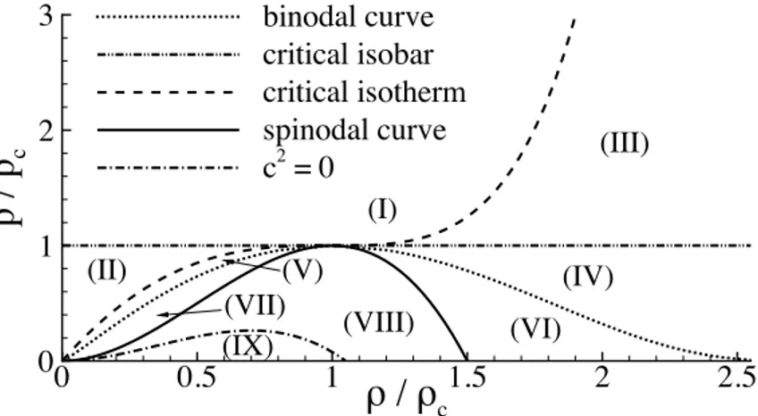
Let us now focus on metastable liquids and liquid-vapor phase transition at constant temperature (cavitation). Figure1.3 provides the phase diagram of a Lennard-Jones fluid [75] with binodal and the spinodal lines reported in the inset. In the ⇢ ✓ plane, the binodal line is identified as the set of points having same temperature, chemical potential and pressure, blu and azure lines in the inset. The spinodal points are identified along isotherms where @p/@⇢ = 0. They are represented by the red and orange lines. All the states

ρ

p

0.1 0.2 0.3 0.4 0.5 0.6 0.05 0.1 0.15 0.2 0.25 isotherm iso-chemical potential ρ_{V spin} ρ_{V sat} ρ_{L spin} ρ_{L sat} ρ θ 0.2 0.4 0.6 0.8 0.7 0.8 0.9 1 1.1 1.2 1.3 ρ_{V sat} ρ_{L sat} ρ_{V spin} ρ_{L spin}

Figura 1.3: Phase diagram for the Lennard-Jones EoS[75]. In the main plot the isotherm ✓ = 1.25 and the iso-chemical potential µ = µsat with the

sa-turation value are reported with dashed and dash-dotted lines, respectively. The saturation densities are identified as the two points with equal tempe-rature, chemical potential and pressure; the red circle represent the vapor saturation point and the orange circle the liquid one. The other two circles, blue and light blue, represent the spinodal points, vapor and liquid respecti-vely, identified on the isotherm where @p/@⇢ = 0. In the inset the loci of all the saturation and spinodal points at different temperatures are reported in the ⇢ ✓ plane.

in the regions comprised between binodals and spinodals are metastable (i.e. drops and bubbles can nucleate in the metastable regions on the left (vapour) and on the right (liquid) of the diagram, respectively).

Metastable liquid is represented by a point placed between the orange and azure line, and it is separated from its stable state (homogeneous vapor

phase), by an energy barrier that must be surmounted to bring the system in the new phase. This occurs due to thermal fluctuations, which, starting from an ideally homogeneous liquid phase, eventually induce the formation of vapour nuclei. After the nuclei reach a critical size, they start expanding surrounded by their mother phase, in a complex non-equilibrium process, leading the system to decompose in two different phases.

Depending on thermodynamic conditions, the time needed for the occur-rence of a sufficiently intense fluctuation event able to produce a supercritical nucleus can be very long. For this reason, nucleation can be seen as a rare event. The relevance of thermal fluctuations underlines the microscopic na-ture of the phenomenon. However, despite its origin is to be definitely found at the atomistic level, nucleation takes place on temporal scales which, due to the rare event issue, is several order of magnitude greater than the mole-cular characteristic time. Moreover, in many cases the interest is centred on systems of macroscopic size.

The presence of impurities or dissolved gas strongly lowers the energy barrier and facilitates bubble formation. The presence of solid boundaries makes a similar effect. In fact the energy needed to form a vapour bubble on a solid surface depends on the contact angle and, as explained in the next section, it can be considerably lower than it is in a bulk phase. This is the reason why it is so common to observe cavitation in water at pressures considerably larger than the extreme cavitation limit of ultra-pure water which can sustain 1 kbar tensions [10]. Moreover recent experimental works have highlighted how the wettability of ultra-smooth surfaces can strongly influence the onset temperature of pool boiling in superheated liquids [26,

Several theoretical models have been proposed in order to estimate the energy barrier and the nucleation rate, i.e. the number of nucleated bubble per unit time and volume, both in homogeneous and heterogeneous (near extraneous boundaries) conditions. The classical nucleation theory (CNT) [18], poses the basis for the understanding of the phenomena, and it may be easily extended to the non-homogeneous case [147], as recalled in Sec. 1.3. The major contribution to the work to create a vapour bubble into a me-tastable liquid is the positive work needed to create the bubble surface. Its value is related to the surface tension and to the surface extension. The counteracting contribution is the energy released to transform the liquid into the stable vapour phase. Its value is related to the difference between the vapour pressure and the ambient pressure and it is proportional to the bub-ble volume. The (algebraic) sum of these two contributions gives the total work needed to create a bubble of a given radius. At small radii the surface contribution prevails up to a critical bubble radius where the needed work is maximum and then the negative volume contribution becomes stronger and the work start decreasing. This maximum work corresponds to the energy barrier that must be overcome to create a vapor region.

1.3 Classical Nucleation theory

Classical nucleation theory (CNT) [80, 28, 147] provides the fundamental understanding of bubble nucleation in a metastable liquid, both for homoge-nous (bubble forming in the bulk liquid) and heterogehomoge-nous conditions (bub-ble forming in contact with an extraneous phase, typically a solid with given geometry and chemical properties). The simplest example of heterogenous nucleation is a vapor bubble nucleating on a flat solid surface at fixed contact

angle . The free energy of a spherical cup laying on a flat solid wall, ⌦ (R, ) = pVV (R, ) + LVALV (R, ) +

+ SVASV (R, ) + LSALS(R, ) , (1.1)

depends on the vapor-liquid pressure jump p = pV pL(the Laplace

pressu-re), the bubble volume VV, the area of liquid-vapor ALV, solid-vapor ASV and

liquid-solid ALS interfaces and the respective surface energies LV, SV, LS.

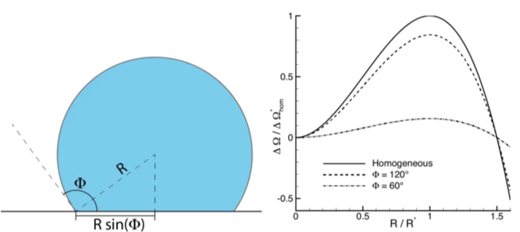
Introducing the equilibrium (or Young) contact angle = cos 1₍ LS SV)/ LV) (see the sketch in Fig. 1.4, where, at variance with the

stan-dard convention, the angle is measured from the vapor-solid interface, i.e. > ⇡/2 means hydrophilic) allows for re-expressing the relevant geometric quantities as ASV = ⇡R2sin2 , ALV = 2⇡R2(1 cos ), ALS = Aw ASV,

VV(R, ) = VV(R, ⇡) ( ), where is Aw the total surface of the solid wall and

( ) = 1/4(1 cos )2_{(2 + cos ). As ! ⇡ the free energy reduces to the}

homogeneous case. Thus, starting from a homogeneous metastable liquid and denoting by ⌦hom = pVV(R, ⇡) + LVALV(R, ⇡) the free energy spent

for a spherical bubble of radius R in the bulk liquid, the energy required to form a spherical cup at the wall reads

⌦ (R, ) = ⌦hom(R) ( ) . (1.2)

The free energy consists of two contribution, one associated with volume terms and decreasing like R3 _{with increasing bubble radius and the other}

depending on the surface area which increases with like the square of the bubble radius. The free-energy attains a maximum, the critical state, at the critical radius R⇤_.

R⇤ = 2 LV

Figura 1.4: Left panel: bubble sketch illustrating the equilibrium contact angle and the bubble radius R. Right panel: CNT prediction of free-energy profiles for different contact angle , the continuous line corresponds to the homogeneous case ( = ⇡), the dotted lines represent the heterogeneous case.

The corresponding free energy barrier is

⌦⇤ = ⌦ (R⇤, ) = ⌦⇤_hom ( ) = 16 3 ⇡

3 LV

p2 ( ) . (1.4)

The critical radius is the same both for heterogeneous and homogenous nu-cleation. On the opposite, the barrier ⌦⇤ _{for heterogenous nucleation is}

lower than ⌦hom ( ( )  1). Clearly, for trivial geometrical reasons, also

the critical volume V⇤ _{= 4/3⇡R}⇤3 _{( )is smaller for the heterogeneous case.}

As an example let us compare the work needed to form a vapour bubble in the bulk of the liquid phase ⌦hom (homogeneous nucleation) with the work

needed to form a vapour bubble on a flat solid surface ⌦het (heterogeneous

nucleation) by assuming, for the sake of simplicity, the contact angle = ⇡/2. It is straightforward to realize that ⌦hom= 2 ⌦het, since the critical bubble

is expected to be a perfect half of the one in homogeneous condition. It follows that the probability of observing a nucleated bubble on a solid surface

is significantly larger than the probability of observing a vapour bubble in the bulk.

1.3.1 The Blander and Katz Nucleation Rates

The crucial observable in the nucleation process is the nucleation rate, i.e. the normalized number of super-critical bubbles formed per unit time. In the heterogeneous context the normalization is per unit surface (as opposed to unit volume used in homogeneous conditions). The expression for the nucleation rates[18, 41] are

JBK = nL r 2 LV ⇡m exp ✓ ⌦⇤ kB✓ ◆ , (1.5)

concerning the homogeneous nucleation, and

JBK = n2/3L (1 cos ) 2 r 2 LV ⇡m exp ✓ ⌦⇤ kB✓ ◆ , (1.6)

for the heterogeneous one, where nL is the liquid number density and m the

mass of the liquid molecule.

Equations (1.5–1.6) represent the famous Blander and Katz expressions for the nucleation rates in the CNT context. They are commonly used as a reference theory in nucleation.

1.3.2 The Kramers theory

Kramers theory [83] provides the mean time ⌧ for the diffusion across a barrier (mean first passage time) of a random walker trapped in the metastable basin of a given potential. Let us denote B ⇢ S the metastable basin where S is the space of the states for the physical system (each trajectory X(t) 2 S).

In the present context the random walker is assumed to obey the Langevin equation

dX

dt = µ (X) + (2D)

1/2_{⇠(t) , (1.7)}

where ⇠ is delta-correlated process, h⇠(t) ⌦ ⇠T_(t0

)_{i = (t} t0) with D the diffusion tensor. Let us denote P (X, t|Y, t0)the transition probability from

the state Y at the time t0 to the state X at the time t. It obeys the Fokker

Planck equation (see Appendix B for details) @P (X, t_{|Y, t}0) @t = FP (X, t|Y, t0) , (1.8) where F = @ @X · µ (X) @ @X ⌦ @ @X : D , (1.9)

is the Fokker Planck operator.

Eq.1.8must be complemented with initial and boundary conditions, that in the context of barrier crossing problems can be assumed to be

P (X, t0|Y, t0) = (X Y) X2 B ,

P (X, t_{|Y, t}0) = 0 X2 @B ,

in other words @B is an absorbing boundary.

The probability that the trajectory X is still contained in the basin B, or equivalently, the probability that the mean first passage time ⌧(Y) (time required to reach @B starting from Y) is greater than the current time t, can be easily evaluated as ⇧ (t_{|Y, t}0) = Z B P (X, t_{|Y, t}0) dX = P r (⌧ (Y) > t) = Z +1 t ⇡ (⌧_{|Y) d⌧ ,} (1.10)

with ⇡ (⌧|Y) the probability density distribution of the first passage times. Thus the mean value of ⌧ is

h⌧ (Y)i = Z +1 0 ⌧ ⇡ (⌧|Y) d⌧ = Z +1 0 ⌧ @⇧ (⌧|Y, 0) @⌧ d⌧ , (1.11)

that, after integrating by parts provides

h⌧ (Y)i = Z +1 0 d⌧ Z B P (X, ⌧_{|Y, 0) dX .} (1.12) Since Y is the starting state for the random walker X, the governing equation for the mean first passage time, will be related to the Kolmogorov Backward equation, in fact by applying the adjoint of the operator F to the Eq. 1.12

one finds F†h⌧ (Y)i = Z +1 0 d⌧ Z B @P (X, ⌧|Y, 0) @⌧ dX , (1.13)

where Eq. C.13in Appendix B has been enforced, and the stationary condi-tions are invoked P (X, t|Y, t0) = P (X, t t0|Y, 0). So, the Eq. 1.13can be

integrated, by using Eq. 1.10 leading to

F†h⌧ (X)i = 1 , (1.14)

representing a differential equation for the mean first passage time, with the boundary condition h⌧ (X)i = 0 on @B.

In the light of above general description, for a one dimensional physical system, moving in a bistable potential ⌦(X), according to the equation

dX dt = d⌦ dX + p 2D⇠(t) , (1.15)

a simple equation for h⌧i can be deduced by enforcing Eq. 1.14, d⌦ dX d dXh⌧ (X)i + D d2 dX2h⌧ (X)i + 1 = 0 , (1.16)

By multiplying both sides of Eq.1.16by the integrating factor exp( ⌦)/D, the equation is rearranged as

d dX ✓ exp ( ⌦)dh⌧(X)i dX ◆ = 1 Dexp ( ⌦) , (1.17) with = 1/kB✓.

Hence by initialising the system in the metastable basin [, the mean time required to reach the saddle point in the unstable basin \, is obtained by integrating Eq. 1.17, leading to

h⌧i = Z [ exp ✓ ⌦(X) kB✓ ◆ dX Z \ 1 Dexp ✓ ⌦(X) kB✓ ◆ dX . (1.18)

The relationship between barrier crossing and nucleation, becomes evident when one considers the free energy of a vapor bubble in a surrounding liquid, as prescribed by CNT. In fact by imposing the potential ⌦ = ⌦ in Eq.1.2, the mean time required to form a critical bubble can be evaluated by solving Eq. 1.18.

Here for the sake of simplicity a simple approximation of Eq. 1.14 based on the Laplace’s method is reported. This method provides accurate results for high barriers. Alternatively a numerical approach should be adopted. The approximation is ⌧ = 1 D⇤ exp ✓ ⌦⇤ kB✓ ◆ Z +1 1 dr exp ✓ 1 2 kB✓ r2 ◆ 2 , (1.19) with = d2 _⌦/dR2_|

R=0 = 8⇡ LV ( ). The RHS of Eq. (1.19) is a Gaussian

integral that is easily calculated providing ⌧ ( ) = 1 D⇤ kB✓ 4 ( ) LV exp ✓ ⌦⇤ kB✓ ◆ . (1.20)

The diffusion coefficient D⇤ _{= k}

B✓/16µ⇡R⇤ as evaluated in [101], by

enfor-cing the fluctuation dissipation balance for the overdamped Rayleigh-Plasset equation, where µ is the fluid viscosity.

Once ⌧ is evaluated, the nucleation rate may be estimated as [12, 55]

Jhom=

nL

⌧ (⇡) , (1.21)

for the homogeneous case, and

Jhet =

n2/3_L

⌧ ( ) , (1.22)

for the heterogeneous one.

1.4 Modelling Thermal Fluctuations at the

Con-tinuum Level

As discussed in the previous sections, a suitable modelling of thermal fluctua-tions is crucial to address nucleation, and in general multiphase flow involving spontaneous phase transformations. For this reason a brief description of the theory of hydrodynamic fluctuations at the continuum level is included in the present Introduction.

At the molecular scale, even in conditions of thermodynamic equilibrium, the fluids exhibits a stochastic behaviour. In fact, going down below the micrometer scale, the effects of thermal fluctuations play a dominant role in the dynamics of the system. As a consequence, a suitable description of me-soscale fluid dynamics must include thermal fluctuations. Such fluctuations have been experimentally investigated by light and neutron scattering [15]. Since the pioneering work of Landau and Lifshitz (1958, 1959) [84] several models, describing the hydrodynamic fluctuations at the continuum level, have been developed [61, 152, 104, 124]. In the literature these approaches are grouped under the name of "Fluctuating Hydrodynamics". The main

idea of Lifshitz and Landau theory is to treat the thermodynamic fluxes as stochastic processes. As prescribed by the thermodynamics of irreversible processes, at macroscopic level, thermodynamic fluxes are the expression of microscopic molecular degrees of freedom of the thermodynamic system. Un-der this respect dissipation in fluids can be seen as macroscopic manifestation of the energy transfer arising from random molecular collisions [40]. Thus at mesoscopic scale, thermodynamic fluxes have to be modeled as stochastic tensor fields, whose statistical properties can be inferred by enforcing the fluctuation-dissipation-balance (FDB). Since the eminent work of Einstein on the theory of equilibrium thermal fluctuations [57], other investigators have analised the statistical fluctuation by considering the entropy as the proba-bility functional of the fluctuations [61, 123, 124]. Each fluctuation results in an entropy deviation from the equilibrium value (the maximum value). Evidently, every large deviation from the equilibrium conditions (resulting for a great fluctuation) will have a very small probability of occurrence.

Once a suitable probability distribution functional of the fluctuations is available, a stochastic process reproducing such equilibrium statistical pro-perties can be appropriately defined. In this context, the fluctuating hydro-dynamics equations can be seen as a set of stochastic processes reproducing the Einstein-Boltzmann probability distribution for the fields, whose deter-ministic part is represented by the Navier-Stokes equations. In principle the theory of fluctuating hydrodynamics has been derived for the linearised Navier-Stokes equations, and as such, it can be considered valid only for small fluctuations. However some important works have advanced the theo-ry to the non-linear regime [132, 133, 142], highlighting several differences with respect to the linear one. In particular the study of one dimensional

non-linear stochastic Burgers equations provides connections with the KPZ scaling behavior [78], and the Levy distribution. In addition, non-linear ver-sion of FDB are well know [136], as well as stochastic equations for non-linear hydrodynamics [59]. These theories, far away from equilibrium, provide cri-tical changes in the field statistics, resulting in long-ranged correlations also in stationary non equilibrium conditions, like, e.g. in the Rayleigh-Bernard problem [39]. More commonly, the extension of the theory to the non-linear case, is based on the assumption on the local-equilibrium [21, 40]. This as-sumption implies that in a non-equilibrium condition, the expressions for the fluctuation statistics of a system in equilibrium continue to be valid, by sub-stituting the equilibrium values with the local values of the hydrodynamic fields. Starting from the pioneering work of Garcia et al. [65], in recent years there has been an exponential increase of numerical methods for fluctuating hydrodynamics equations [54, 46, 11, 53, 13]. These models not only play an important role in the physics of fluids, but their predictive power can be useful to improve some of the latest nanotechnologies. For instance the mo-deling of thermal fluctuations is crucial in the design of flow micro-devices [47,20], in the study of biological systems, such as lipid membranes [107], in the theory of Brownian engines and in the development of artificial molecular motors prototypes [115]. Inspired by organic devices able to convert chemi-cal into mechanichemi-cal energy by means of thermal noise, devices operating with the same principles have been theorised. For instance, the cell division is a mechanical process, driven by the chemical energy released during the ATP hydrolysis , with much higher efficiency than the common operating machi-nes. Actually RNA and DNA polymerase can be seen as molecular motors. In addition, thermal fluctuations play also an important role in the breakup

of droplets in nano jets [105, 56,77].

1.5 Beyond Classical Nucleation Theory

In the previous sections, the main features of nucleation have been described, highlighting the fundamental physical aspects. The CNT poses the founda-tions for basic understanding, however it still lacks some crucial features. More sophisticated theories like density functional theory (DFT) [113, 91], interesting extensions [95, 101], and molecular dynamics (MD) simulations can give more precise estimates of the barriers and can correct some mis– prediction of CNT. Such methods are extremely powerful in stationary condi-tions and need to be coupled to specialized techniques, like the string method [148], to study the nucleation events and the transition path [67].

Often, depending on the thermodynamic conditions, the time to be awai-ted to observe the nucleation event is so long and its probability is so small that the phenomenon is labeled as a “rare events”. In particular this time grows exponentially as the energy barrier [83]. For this reason, in the last decades there have been several works addressing nucleation by the means of rare-event techniques [3, 4, 22, 42]. Forward Flux Sampling (FFS) explores a series of interfaces placed between an initial and final states to calculate rate constants and transition paths, both in equilibrium and nonequilibrium systems driven by stochastic dynamics. Transition Path Sampling (TPS) perturbs random paths in the space of configurations –as in Monte Carlo walks– by accepting or rejecting configurations to reconstruct the correct path probability. Alternatively the study of nucleation processes is almost uniquely addressed by direct molecular dynamics simulations [6, 49], which for a large part of the real systems are often computationally too expensive,

limiting its application to very small domains, often far from the technologi-cal applications. In addition molecular dynamics simulations are not able to capture the hydrodynamics effects, crucial for the next phases of the nuclea-tion process. These aspects suggest the adopnuclea-tion of mesoscale models for the study of nucleation in its entirety, starting from the phase change inception up to the macroscopic motion.

Promising approaches are based on phase field models, having as order parameter the mass density itself. In stationary conditions they recover the DFT descriptions with a squared-gradient approximation of the excess energy [92]. The phase field models have the advantage of being easily extended to unsteady situations, enabling the full description of both the thermodynamic and the fluid dynamics fields [96, 99, 97]. The model, in its original form, is deterministic and cannot capture spontaneous nucleation originated by thermal fluctuations, in absence of external forcing. To this purpose, the theory of fluctuating hydrodynamic [40,33] represents the natural framework to embed thermal fluctuations inside the phase field description, and also it has been recently stressed as the theory can be used to formulate dynamical theory of nucleation [93], providing stochastic equations for the evolution of order parameter and a formalism to evaluate the nucleation pathways.

During my PhD research, I developed a novel mesoscale approach, based on a diffuse interface description of the two-phase vapor-liquid system em-bedded with thermal fluctuations through a fluctuating hydrodynamics mo-deling. The model has been used to address vapor bubble nucleation in both homogeneous [63,64] and heterogeneous case (see Chapter 7). This mesosca-le approach offers a good mesosca-level of accuracy (as exposed in the next sections) at a very cheap computational cost compared to other techniques, providing

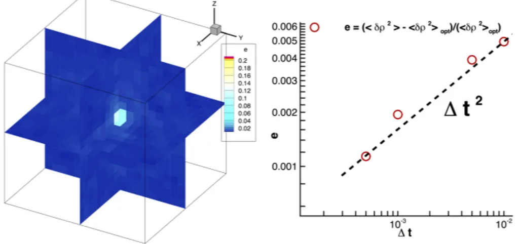
the possibility of dealing with macroscopic system. The typical size of the simulated system on a small computational cluster (200⇥200⇥200 nm3_,

cor-responding to a system of order 108 _{atomistic particles) is comparable with}

one of the largest MD simulations [49] on a tier-0 machine. Moreover the simulated time is here Tmax ⇠ µs to be compared with the MD Tmax ⇠ ns.

The enormous difference between the two time extensions allows us to ad-dress the simultaneous nucleation of several vapor bubbles, their expansion, coalescence and, at variance with most of the available methods dealing with quasi-static conditions, the resulting excitation of the macroscopic velocity field. These hydrodynamic effects –not easily detectable with conventional techniques– have a great influence on the nucleation dynamics, specially for closed systems [63], where "bubble crowding" strongly affects the nucleation rate. The above approach has been extended also to address heterogeneous vapor bubble nucleation, showing its applicability even when dealing with more complex physical systems, e.g., vapor bubble nucleation on solid surface having different wetting properties (see Chaper 8).

Capitolo 2

Diffuse interface models

Aim of this chapter is to introduce the diffuse interface approach that will be exploited in the present thesis. The chapter will start discussing the general thermodynamic description of the two-phase, liquid-vapour systems, and will analyse with great detail the particular case of the Van der Waals model, the so-called “square-gradient approximation”. The resulting model provides a mesoscale description of the liquid-vapour system, enabling a robust charac-terisation of the interfacial properties, namely the interface thickness and the surface tension, down to the nanometer length scale.

The presence of a confining solid surface with different wetting properties can be also taken into account with this approach. In this context I propose a general expression to uniquely identify the solid-fluid contact angle, rela-ting the solid-fluid free energy contributions with the bulk properties of the fluid. This model recovers the classical Young-Laplace equilibrium wetting condition and the prescribed expressions for the diffused contact line in the context of the famous Cahn-Hilliard phase field approach for binary flows. Successively, the governing equation of multiphase systems enodowed with capillarity will be derived in details, by choosing a thermodynamic consistent

constitutive relationship between thermodynamic forces and thermodynamic fluxes. During my research I exploited this model to address the collapse of a cavitation bubble near a solid boundary, showing an unprecedented descrip-tion of interfacial flows, that naturally takes into account topology modifica-tion and phase changes (both vapour/liquid and vapour/supercritical fluid transformations).

In order to deal with the rare event issue described in the Introduction which, of course, is still present in the proposed mesoscale description, the diffuse interface model will be coupled with the string method, one of the specialised rare event techniques, in order to extract the free energy barriers and the transition paths during both homogeneous and heterogeneous vapour bubble nucleation.

2.1 Thermodynamic of non-homogeneous systems

Let us briefly describe the thermodynamic equilibrium of a two-phase sy-stem, focusing on a closed system with fixed temperature and volume. Van der Waals was the first to recognise that a description of the Helmholtz free energy based only on the local values of temperature and phase indicators was not sufficient to describe the internal structure of a transition zone se-parating two different phases. Indeed he showed how a local description of the free energy provides a separating interface having zero-thickness and zero surface tension. Thus, in order to describe to thermodynamics of a non-homogeneous system, in which the different phases are separated by a smooth transition zone, a non-local term (depending on the spatial gradients of the phase indicator) should be added to the free energy of the system. In modern terminology, the non-local terms in the free energy can be justified in

the context of Density Functional Theory, see Lutsko ([91,92]) for a detailed derivation and related comments. Accounting for the presence of a solid wall in contact with the fluid, the general form of the (Helmholtz) free-energy functional F as a function of the temperature ✓ and a phase indicator takes the form

F [ , ✓] = Z V fb( , ✓) + fs(r , ..., r ⌦ ... ⌦ r ) dV + Z @V fw( , ✓) dS , (2.1) where fb is the homogeneous bulk free-energy contribution, fw is related to

solid-fluid interactions and fs is the gradient contribution, depending on the

spatial gradients of the phase indicator . At fixed temperature ✓ = ✓0 the

equilibrium condition is reached when the first variation of the functional 2.1

with respect to the phase indicator is zero, leading to the Euler-Lagrange equation F = @fb @ + N X k=1 ( 1)k_r(k) : @fs @⇣_r(k) ⌘ = 0 , (2.2) where the superscript ⇤(k) _{on the differential operator r denotes rank k}

ten-sor operator defined as the n-fold tenten-sor product of r with itself. Eq.2.2is a partial differential equation for the equilibrium profile of the phase indicator

with boundary conditions @fw

@ + g (r , ..., r ⌦ ... ⌦ r , n) = 0 , (2.3) with n as a unit normal on the domain V and g is a function arising from the boundary terms when integrating by parts. The boundary conditions arise, in fact, from the extremality condition on the free-energy functional, due the

presence of the solid-fluid interactions described by the free-energy boundary term.

It is worth stressing that the existence of a smooth equilibrium configu-ration eq of two distinct phases, i.e. a diffuse interface separating them,

originates from the presence of the gradient contribution to the free energy.

2.2 The Van der Waals approach

In the last part of XIX century scientists were starting to recognise that the separation surface between two thermodynamic phases could have a finite thickness. Van der Waals, based on phenomenological assumptions, proposed a gradient theory that led him to predict the interface thickness of a fluid near the critical point. In the framework of a general phase field theory, Van der Waals assumes the density field as the relevant phase indicator, and the density gradient square norm as a surface contribution basically localised at the liquid-vapour interface where the density gradient is large (see. Eq. 2.4

below). The model is extremely powerful both for steady and unsteady conditions, providing a robust description of interfacial flows that naturally accounts for topology modification of the regions occupied by the two phases and the phase change between them [96,98]. Since in this initial illustration of the model the focus is on the properties of the fluid irrespective of the solid walls it may be in contact with, like e.g. surface tension, interface thickness and the constitutive relationship for thermodynamic fluxes, for the time being the solid-liquid free energy contribution is neglected. It will be taken up again in some detail in the forthcoming sections.

For a closed system, with a given mass M0, the constrained Helmholtz

[45, 72, 5] is: Fc[⇢, ✓] = F [⇢, ✓] + l ✓ M0 Z V ⇢dV ◆ = Z V f dV + l ✓ M0 Z V ⇢dV ◆ = = Z V ✓ fb(⇢, ✓) + 2r⇢ · r⇢ ◆ dV + l ✓ M0 Z V ⇢dV ◆ , (2.4) where l is a Lagrange multiplier, f = fb+ /2|r⇢|2 with fb(⇢, ✓) the

classi-cal Helmholtz free energy density per unit volume of the homogeneous fluid at temperature ✓ and mass density ⇢. The coefficient (⇢, ✓), in general a function of the thermodynamic state, embodies all the information on the interfacial properties of the liquid-vapour system (i.e. surface tension and in-terface thickness). At given temperature, equilibrium is characterized by the minimum of the free energy functional (2.4), where variations are performed with respect to the density distribution ⇢ assumed to be the proper phase de-scriptor for the liquid-vapour phase transition. The relevant Euler-Lagrange equation is

µb_c r · ( r⇢) l = 0 , (2.5)

where the temperature is constrained to be constant, ✓ = const, µb

c =

@fb/@⇢|✓ is the classical chemical potential, and the Lagrange multiplier is

identified as l = µb

c r · ( r⇢) = µc(⇢eq) = µeq evaluated at the

equili-brium density field. The equation defines a generalised chemical potential µc = µbc r · ( r⇢) that must be constant at equilibrium.

The consequence of the above equilibrium conditions is better illustrated in the simple case of a single planar liquid-vapour interface separating the two bulk, homogenous phase (liquid and vapour, respectively). The only direction of inhomogeneity is s and a constant is assumed. The constant temperature appears in the problem as a parameter and will not be further mentioned

throughout the present section. Hence, determining the equilibrium density distribution amounts to finding a solution of

µc = µbc(⇢)

d2_⇢

ds2 = µeq . (2.6)

The boundary conditions for this second order ordinary differential equation are obtained by evaluating the generalised chemical potential far away on the two sides of the interface, namely in the bulk liquid and bulk vapour where d⇢/ds = 0. It follows µeq = µbc(⇢V) = µbc(⇢L).

The solution of Eq. (2.6) is readily obtained by multiplying through by d⇢/ds and integrating between ⇢1 = ⇢V and ⇢,

wb(⇢) wb(⇢V) = 2 ✓ d⇢ ds ◆2 , (2.7)

where wb(⇢) = fb(⇢) µeq⇢. Equation (2.7) shows that wb has the same

value in both the bulk phases, where the spatial derivative of mass density vanishes: wb(⇢L) = wb(⇢V).

The grand potential, defined as the Legendre transform of the free energy, ⌦ = F Z V ⇢ F ⇢dV = Z V wdV , (2.8)

has the density (actual grand potential density)

w[⇢] = f µc⇢ = fb+ 2 ✓ d⇢ ds ◆2 ✓ µb_c d 2_⇢ ds2 ◆ ⇢ , (2.9)

implying that, in the bulk, w = wb, i.e. wb is the bulk grand potential density.

Given the form of wb(⇢), the solution of Eq. (2.7) provides the (implicit

expression for the) equilibrium density profile ⇢(s):

s = r 2 Z ⇢ ⇢v d⇢ p wb(⇢) wb(⇢V) + const . (2.10)

Eq. (2.10) provides the equilibrium density profile characterized by two bulk regions separated by a thin layer. The layer thickness can be estimated as

✏ = ⇢L ⇢V d⇢/ds|max

. (2.11)

The equilibrium condition, Eq. (2.7), provides the interface thickness in terms of the bulk grand potential density wb(⇢)and of the parameter ,

✏ = (⇢L ⇢V)

s

2 [wb(¯⇢) wb(⇢V)]

, (2.12)

without explicitly addressing the density profile. ¯⇢ is the density correspon-ding to the maximum of d⇢/ds, achieved where dwb/d⇢ = 0, in Eq. (2.7).

The surface tension can be defined as the excess (actual) grand potential density, = Z Si 1 (w[⇢] w[⇢V]) ds + Z ₁ Si (w[⇢] w[⇢L]) ds = (2.13) = Z 1 1 (w[⇢] w[⇢V]) ds,

where Si is the position of the Gibbs dividing surface, whose precise value

is ininfluential since w[⇢V] = w[⇢L] (we stress that, e.g., w[⇢V] should be

interpreted as the functional (2.9) evaluated at the constant density field ⇢V). Given the definition of w[⇢], Eq. (2.9), and exploiting the equilibrium

condition for the chemical potential, Eq. (2.6), it follows that = Z 1 1 " fb + 1 2 ✓ d⇢ ds ◆2 µeq⇢ wb(⇢V) # ds = (2.14) = Z ₁ 1 " wb + 1 2 ✓ d⇢ ds ◆2 wb(⇢V) # ds .

Using Eq. (2.7) one finds = Z +1 1 ✓ d⇢ ds ◆2 ds = Z ⇢L ⇢V d⇢ dsd⇢ = (2.15) = Z ⇢L ⇢V p 2 (wb(⇢) wb(⇢V)) d⇢ ,

where the second expression can be evaluated with no a priori knowledge of the equilibrium density profile. It worths stressing that, as for the interface thickness, the surface tension only depends on the form of the bulk grand po-tential density wb(⇢)in the density range between the two equilibrium values,

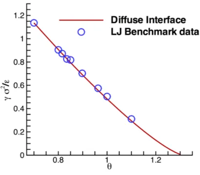
[⇢V; ⇢L], and on the parameter . Figure2.1 reports the comparison between

the diffuse interface prediction of surface tension and molecular dynamics simulations, for a Lennard-Jones fluid. A constant value of was assumed to reproduce the simulation data. It is evident how the Van der Waals model is able to capture the temperature dependence of surface tension. Of course, equation (2.7) applied to the two adjoining bulk regions where d⇢/ds = 0 implies the mechanical equilibrium condition p(⇢L) = p(⇢V), where

p = @ ˆfb @v = @fb/⇢ @v = ⇢µ b c fb (2.16)

is the classical thermodynamic pressure, ˆfb = fb/⇢ the specific bulk free

energy, and v = 1/⇢ the specific volume. Indeed Eq. (2.7) implies wb(⇢V) =

wb(⇢L), which corresponds to the equality of the pressures given that p =

wb.

2.3 Solid-Fluid Free Energy

In order to describe a non-homogeneous liquid-vapour system interacting with a solid surface, I again start from the Van der Waals square gradient approximation of the (Helmoholtz) free energy functional,

Figura 2.1: Comparison between the temperature dependen-ce of the surfadependen-ce tension obtained through Eq. (2.15), when using the Lennard-Jones EoS [75], and the benchmark data provided at the url https://www.nist.gov/mml/csd/chemical-informatics-research-group/lennard-jones-fluid-properties. The value of the capillary coefficient is fixed to m2_/( 5_{✏) = 5.224. The results are presented in a non-dimensional}

Figura 2.2: Bubble sketch illustrating both geometrical and wetting properties. Fc[⇢, ✓] = Z V dV ✓ fb(⇢, ✓) + 1 2 r⇢ · r⇢ ◆ +l ✓ M0 Z V ⇢dV ◆ + Z @V dSfw(⇢, ✓) . (2.17) For the sake of uniformity with the previous section, I address the equilibrium problem in the canonical ensemble, i.e. at constant mass, volume and tem-perature, but the generalization to the microcanonical ensemble (constant mass, volume, energy) is straightforward and is addressed in Chapter 8. By minimising the free-energy, it follows that, in equilibrium, temperature and (generalized) chemical potential µc must be constant, as expected,

✓ = const = ✓eq (2.18)

Furthermore the boundary term gives rise to the additional requirement ✓ r⇢ · ˆn + @fw @⇢ ◆ @V = 0 , (2.20)

where ˆn is the outward normal, to be read as a (non-linear) boundary condi-tion for the density. The free energy contribucondi-tion fwarises from the fluid-wall

interactions and accounts for the wetting properties of the surface. In order to come up with a model fw, I deduced an analytic form that generalises an

approach that has been already used to describe two immiscible fluids, see e.g [126, 71].

The analytic form of fw is constructed by observing that the equilibrium

contact angle is related to the inhomogeneity direction ˆs as ˆs· ˆn = cos , (see Fig. 2.2), and the density gradient is r⇢ = d⇢/ds ˆs, so that Eq. 2.20

reads

dfw

d⇢

d⇢

ds cos = 0 , (2.21)

the above equation can be integrated by using Eq. 2.7 providing fw(⇢) = cos

Z ⇢ ⇢V

p

2 (wb(˜⇢) wb(⇢V)) d˜⇢ + fw(⇢V) . (2.22)

The analytic form of fw recovers the physical evidence that for a pure vapor

of density ⇢V in contact with the wall, the free-energy should be given by

the solid-vapor surface tension, fw(⇢V) = SV. Similarly, for a pure liquid

of density ⇢L, fw(⇢L) = LS. These aspects become even more evident by

enforcing Eq. 2.15, leading to

fw(⇢L) = LS = LV cos + SV , (2.23)

the famous Young equilibrium wetting condition.

Using the expression (2.22), @fw/@⇢ ⌘ 0 in both stable liquid and

derivative for the density outside coexistence and metastable regions and assigning the contact angle otherwise, i.e. in the small region where the finite thickness liquid-vapour interface meets the wall. In fact Eq. (2.21) pro-vides a uniquely defined relationship between contact angle and the normal derivative of the density, confirming that the surface energy fw encodes the

wetting properties of the wall. In addition, when a pure liquid in metastable state is in contact with the wall, the model provides a wall normal strati-fied density profile, in which the density is higher toward the solid surface, for a hydrophilic wall, and is lower for a hydrophobic one. In Fig. 2.3 the equilibrium density profiles are reported as a function of the wall normal z, showing the depletion or absorption layering of the liquid in proximity of the solid surfaces, as commonly detected [34,74] in MD simulations. As evident, the density profiles are not monotonic, foretelling the existence of an exten-ded region near walls where ⇢(z) < ⇢b for hydrophilic interactions ( > ⇡/2)

and ⇢(z) > ⇢b for hydrophobic ones. Such behaviour is consistent with the

constant mass constraint which characterises closed systems. These aspects play an important role in heterogeneous nucleation, inasmuch bubble forma-tion is favoured on hydrophobic walls and discouraged on hydrophilic ones. Such qualitative statement is corroborated both by energetic considerations and by fluctuating hydrodynamics simulations of spontaneous heterogeneous bubble nucleation to be discussed in forthcoming sections (see Chapter 8).

2.4 The String method: energy barriers and

the critical bubble

During my PhD research, I coupled the diffuse interface description together with a rare-event technique (the string method), in order to obtain the

cri-z/L

z

ρ

/ρ

b 0 0.2 0.4 0.6 0.8 1 0.97 0.98 0.99 1 1.01 1.02 _{φ= 100}0 φ = 800 φ = 1200 φ = 600

Figura 2.3: Spatial density distribution in wall normal direction z. The den-sity values are normalized with mean bulk denden-sity ⇢b, the normal coordinate

z is normalized with the total domain lenght Lz. Two walls with the same

wetting properties are located at z = 0 and z = Lz. The different profiles

refer to different contact angle .

tical configurations of the bubbles both in homogeneous and heterogeneous nucleation. The procedure was successfully exploited by Ren [122] to study the wetting transition on structured hydrophobic walls for a Cahn-Hillard binary fluid. In this work, it is extended to study vapour bubble nucleation, for a Van der Waals diffuse interface model.

The minimisation of the free energy functional (2.4), stating that the ge-neralised chemical potential µc = µbc(⇢) r2⇢ must be constant and equal

to the external chemical potential µext, allows the evaluation of the

thermodynamic conditions where either the liquid or the vapour are stable, constant chemical potential corresponds to a homogeneous phase. When the liquid or the vapour are metastable instead three solutions at constant che-mical potential are found: i) the homogeneous vapour; ii) the homogeneous liquid; iii) a two-phase solution with a spherical (critical) nucleus of a given radius (vapour/liquid in the case of bubble/droplet, respectively), the critical nucleus being surrounded by the metastable phase.

Dealing with nucleation, the non-trivial solution of case (iii), ⇢(r) = ⇢crit(r) where the critical bubble is surrounded by the metastable liquid at

⇢ = ⇢met

L , ✓ = ¯✓and µc(⇢metL , ¯✓) = µmetis particularly significant. The solution

⇢(r) = ⇢crit(r)is found by solving the non linear Euler-Lagrange equation of

the functional 2.4 which, in spherical coordinates and at fixed temperature, reads µb_c(⇢, ¯✓) r2 @ @r ✓ r2@⇢ @r ◆ = µmet. (2.24)

The critical bubble, ⇢c(r), is an unstable solution of Eq. (2.24) which requires

specialised numerical techniques. In this work the powerful string method is applied [149] which, as additional information, identifies the minimum energy path (MEP) joining the metastable fluid (e.g. the liquid) to the fluid (e.g. the vapour ensuing form cavitation). Since our interest here in mainly on cavitation, the problem is specified as a liquid in metastable conditions inside a domain of fixed volume. The stable state will correspond to the presence of an equilibrium bubble enclosed by the liquid contained in the domain. Please note that at fixed volume, mass and temperature the stable state is in fact a vapor bubble surrounded by the liquid phase. The MEP can be visualised as the continuous sequence of density configurations, ⇢(r, ↵), the system assumes when transitioning from the metastable to the stable state,

where ↵ is a suitably defined parameter along the path. The distance between two configurations is expressed as

` = s 1 V Z ⇢2_(r)dV (2.25)

and defines the arclength along the path. The discrete form of the path, consisting of a finite number of configurations, is called the string. The string method numerically approximates this path starting from an initial set of Ns configurations {⇢k(r)}. The head of the string (k = 1) is initialised

as a uniform density field corresponding to the uniform metastable liquid ⇢(r) = ⇢met

L ; the tail (k = Ns) is initialised as a guessed tanh-density profile

adjoining the liquid and the vapour density to approximate a vapour bubble. All the intermediate images on the string are obtained by interpolation of these two density fields with respect to the above defined arclength. The algorithm used for relaxing the string to its final configuration, follows two steps:

1) All the images ⇢k_{(r)are evolved over one pseudo-time-step ⌧ following}

the steepest-descent algorithm (over-damped regime) @⇢ @⌧ = µ met  µb_c(⇢) r2 @ @r ✓ r2@⇢ @r ◆ . (2.26)

2) The images are redistributed along the string following a reparametri-zation procedure by equal arclength. The algorithm is arrested when the string converges within a prescribed error.

It is worthwhile noting that the transition path geometry depends in general on the relaxation dynamics used to evolve the string. In an over-damped re-gime, steepest descent relaxation (Eq. 2.26), could still be used as a reference

theory, as often done in the current literature. In this context the string con-verges to the MEP connecting the local minimum to the saddle point, that under the above assumption is also the most probable transition path [122] . However critical cluster as well as the energy barriers do not depend on the relaxation dynamics. The density profile of the critical nucleus, plotted in panel of Fig. (2.4) at different metastable conditions, allows the evaluation of the critical radius, by following the relation [44]

R⇤ = Z 1 0 r(@⇢c/@r)2r2dr Z 1 0 (@⇢c/@r)2r2dr , (2.27)

and the evaluation of the energy barrier ⌦⇤ = Z 1 0 f (⇢c(r)) f (⇢metL ) µmet ⇥ ⇢c(r) ⇢metL ⇤ 4⇡r2dr , (2.28) defined as the difference in grand potential ⌦ between the critical nucleus and the metastable liquid.

The results of the string method are compared in Tab. 2.1 with tho-se obtained by classical nucleation theory (CNT) which yields the estimate

⌦⇤CNT = 4/3⇡ R2

c. The data show that CNT underestimates the energy

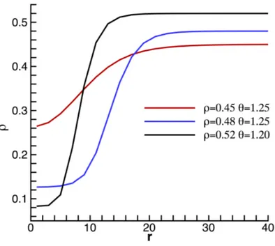
barrier at high temperature while overestimates it near the spinodal [31]. In Fig.2.4the critical density profiles as evaluated from the string method are reported for different temperatures. In The thermodynamic conditions considered here a significant zone of transitions is detected, confirming the importance of considering a phase field approach when dealing with phase transitions, specially for high temperatures and near spinodal conditions. In addition, the energy landscape for a specific thermodynamic condition ⇢L =

Figura 2.4: Density profiles of the critical nuclei, evaluated with the string method, at different thermodynamic conditions of the metastable liquid. The results are presented in a non-dimensional form, taking as reference values the Lennard-Jones parameters.