DiSES Working Papers
Università degli Studi di Salerno Dipartimento di Scienze Economiche e Statistiche >>>www.dises.unisa.it
GRID for model structure discovering
in high dimensional regression
Francesco Giordano
Soumendra Nath Lahiri
Maria Lucia Parrella
ISSN: 1971-3029
Dipartimento di Scienze Economiche e Statistiche Università Degli Studi di Salerno
Via Ponte Don Melillo – 84084; Fisciano (SA) – Italy
Tel +39-089-96.21.55 Fax +39-089-96.20.49 E-mail [email protected]
GRID FOR MODEL STRUCTURE DISCOVERING IN HIGH DIMENSIONAL REGRESSION
Francesco Giordano∗ Soumendra Nath Lahiri† Maria Lucia Parrella‡
Abstract. Given a nonparametric regression model, we assume that the number of covariatesd → ∞ but only some of these covariates are relevant for the model. Our goal is to identify the relevant covariates and to obtain some information about the structure of the model. We propose a new nonparametric procedure, called GRID, having the following features: (a) it automatically identifies the relevant covariates of the regression model, also distinguishing the nonlinear from the linear ones (a covariate is defined linear/nonlinear depending on the marginal relation between the response variable and such a covariate); (b) the interactions between the covariates (mixed effect terms) are automatically iden-tified, without the necessity of considering some kind of stepwise selection method. In particular, our procedure can identify the mixed terms of any order (two way, three way, ...) without increasing the computational complexity of the algorithm; (c) it is completely data-driven, so being easily implementable for the analysis of real datasets. In particular, it does not depend on the selection of crucial regularization parameters, nor it requires the estimation of the nuisance parameterσ2(self scaling). The acronym GRID has a twofold
meaning: first, it derives from Gradient Relevant Identification Derivatives, meaning that the procedure is based on testing the significance of a partial derivative estimator; second, it refers to a graphical tool which can help in representing the identified structure of the regression model. The properties of the GRID procedure are investigated theoretically. Keywords: Variable selection, model selection, nonparametric model regression. AMS 2010 classifications: 46A03, 62A01, 60F05.
JEL classifications: C14, C15, C18, C88.
1. Introduction
Nonparametric methods are particularly useful in the preliminary stage of data analysis, for example to make variable selection, model structure discovering and goodness-of-fit tests. In fact, while a correctly specified parametric model is characterized by precise in-ference, a badly misspecified one leads to inconsistent results. On the other side, nonpara-metric modelling is associated with greater robustness and less precision. But a criticism often made to the nonparametric procedures is that they are time-consuming and not “user-friendly”, because their performance depends crucially on some regularization parameters which are difficult to set. This remarkably affects the potentialities of such procedures. To promote the use of nonparametric approaches, the procedures should be automatic and
∗
UNISA - DISES, Via Ponte Don Melillo, 84084, Fisciano (SA), Italy, [email protected]
†NCSU Statistics Department, Campus Box 8203 Raleigh, NC 27695-8203, USA,
‡
easy to implement. At the same time, they should assure the oracle property under general assumptions. Therefore, these goals will represent the main priority of our analysis.
We consider the following nonparametric regression model
Yt= m(Xt) + εt, (1)
where theXtrepresents the Rd-valued covariates and the errorsεtare i.i.d. with zero mean
and varianceσ2. Herem(Xt) = E(Yt|Xt) : Rd→ R is the multivariate conditional mean
function. The errorsεt are supposed to be independent ofXt. We use the notationX(j)
to refer to the single covariates, forj = 1 . . . , d. We indicate with fX(·) the multivariate
density function of the covariates, having support supp(fX) ⊆ Rd, and with fε(·) the
density of the errors.
We assume that the number of covariatesd → ∞ but only some of these covariates are relevant for model (1). Given that the parametric form of the functionm is completely un-known, our goal is to identify the relevant covariates and to obtain some information about the structure of model (1). We propose a nonparametric procedure having the following features:
(a) it automatically identifies the relevant covariates of model (1), also distinguishing the nonlinear from the linear ones (a covariate is defined linear/nonlinear depending on the marginal relation between the response variable and such a covariate, which corresponds to a relative constant/nonconstant gradient, respectively);
(b) the interactions between the covariates (mixed effect terms) are automatically identi-fied, without the necessity of considering some kind of stepwise selection method. In particular, our procedure can identify the mixed terms of any order (two way, three way, ...) without increasing the computational complexity of the algorithm; more-over, the mixed effect terms are classified as nonlinear mixed effect, if they involve some nonlinear covariates, or as linear mixed effect, if they involve only linear
co-variates;
(c) it is completely data-driven, so being easily implementable for the analysis of real datasets. In particular, it does not depend on the selection of crucial regularization parameters, nor it requires the estimation of the nuisance parameterσ2(self scaling).
The multiple test selection procedure is based on the Empirical Likelihood approach. Under suitable assumptions, our procedure can be applied to high dimension datasets. A screening of the available statistical methods proposed so far can help to highlight the main contributions of our work.
Most of the work has been made in the context of variable selection. There are two main approaches to this problem. Both these approaches consider the estimation of the multivariate regression function contextually to relevant variable selection. The first one is based on the idea of LASSO, using some penalized regressions within additive models (see Radchenko & James (2010), Zhang et al. (2011), Storlie & alt. (2011), among others). The appeal of this approach is the fast rate of convergence, which essentially derives from the imposition of an additive model and other crutial assumptions. On the other side, a serious drawback is given by the computational complexity and the difficulty of implemen-tation on real datasets. The second approach, which has inspired this work, is based on a general regression function of dimensiond, which do not impose any additive restrictions
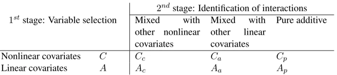
2ndstage: Identification of interactions 1ststage: Variable selection Mixed with
other nonlinear covariates Mixed with other linear covariates Pure additive Nonlinear covariates C Cc Ca Cp Linear covariates A Ac Aa Ap
Table 1: Schematic representation of the GRID procedure. The two dimensions of the table refer to the two stages. The body of the table shows the partition of the regressors Ξ = {1, . . . , d} obtained at the end of the procedure.
on the model (Lafferty & Wasserman (2008)). The main advantage of this approach is its flexibility and simplicity of implementation on real datasets. At the same time, it suffers from a low rate of convergence that makes it unsuitable for the analysis of high dimensional datasets.
Very few papers consider the problem of model selection contextually to variable se-lection, among which Radchenko & James (2010) and Zhang et al. (2011). As far as we know, our procedure is the only one that gives a complete idea of the structure of model (1), without assuming an additive form a priori. As can be seen from points (a)-(c) above, we can derive approximately the exact functional form of the true regression function, which can be used in order to estimate a semiparametric model efficiently.
Our method can be seen as a non trivial extension of the RODEO of Lafferty & Wasser-man (2008), in the sense that we use the same framework and some of the ideas and results presented in their paper, but here we propose a new procedure which also fix some of its drawbacks. Moreover, we perform model selection in addition to variable selection. The acronym GRID has a twofold meaning: first, it derives from Gradient Relevant Identifica-tion Derivatives, meaning that the procedure is based on testing the significance of a partial derivative estimator; second, it refers to a graphical tool which can help in representing the identified structure of model (1). The estimation procedure used in GRID is based on the conjoint implementation of two nonparametric tools: the local linear estimator (LLE) and the empirical likelihood (EL). The peculiarity of our proposal is that it takes advantage of both the strenghts and weaknesses of the two nonparametric tecniques, and it harmonically integrates them in order to pursue the final aim of the estimation.
The rest of this section is devoted to explain how the GRID method works.
Our aim is to classify the covariates of model (1) into disjoint sets: 1) the set of nonlinear
covariates, which includes those variablesX(j)having a nonlinear effect on the dependent variableY (i.e., those with non constant gradient); 2) the set of linear covariates, which includes the variablesX(j)having a linear effect on the response variableY (i.e., constant
gradient); 3) the set of irrelevant covariates, collecting the variables for which the gradient is equal to zero. Denote with C, A and U , respectively, the correspondent index sets and letΞ = C ∪ A ∪ U represent the set of regressors {1, . . . , d}. Secondly, we point to automatically detect the interactions among the covariates, identifying exactly which mixed effects are ‘active’ in model (1). Therefore, each index set can be further partitioned as shown in table 1.
The two dimensions of the table refer to the two stages of the GRID procedure: the first one focuses on variable selection while the second looks at the interaction terms. More
specifically, the information on the interaction terms is given in the following way. Let Ij be the set of covariates mixed with the j-th covariate, for j ∈ Ξ. A convention used here is thatj /∈ Ij, which means that self-interaction is excluded in practice. The GRID
procedure gives a consistent estimation of the setsC and A in the first stage, and the sets Ij in the second stage. The other sets can be derived easily by known relationships. In particular,ICj = Ij ∩ C is the set of nonlinear covariates which are mixed with the j-th
covariate andIAj = Ij∩A is the set of linear covariates mixed with the j-th covariate. Then Ij = Ij C∪ I j A. But alsoCc = ∪j∈CI j C,Ca = ∪j /∈CICj,Ac = ∪j∈CI j AandAa = ∪j /∈CIAj.
All this permits to do variable selection and model structure discovering simultaneously. For example, whend = 10 and the model is
Yt= 2Xt1+ Xt22Xt3+ 10Xt4Xt5Xt6+ exp(Xt7) + εt, (2)
then the first stage of the procedure is devoted to identify the following sets of covariates C = {2, 7}, A = {1, 3, 4, 5, 6}, U = {8, 9, 10},
while the second stage of the procedure identifies the following sets of interactions IA2 = {3}, IC3 = {2}, IA4 = {5, 6}, IA5 = {4, 6}, IA6 = {4, 5}.
To make the GRID procedure ‘user-friendly’, the method is presented in section 5 through a detailed algorithm and the results of the estimation are shown through an intuitive plot which points out clearly both the relevant covariates and their interactions, and helps to write down the (estimated) functional form of the regression functionm(x).
The details are presented in the following sections. Section 2 gives the notation. In section 3 we give the main idea at the basis of the selection procedure. Then, in section 5, we present the test-statistic, the algorithm and the GRID plot. Section 4 describes the multiple testing method, based on the Empirical Likelihood inference. All the proofs are collected in the appendix.
2. Basics of the multivariate local linear estimator
The local linear estimator is a nonparametric tool whose properties have been studied deeply. See Ruppert & Wand (1994), among others. Letx = (x1, . . . , xd) be the
tar-get point at which we estimatem. The LLE performs a locally weighted least squares fit of a linear function, being equal to
arg min β0,β1 n ∑ t=1 {Yt− β0(x) − β1T(x)(Xt− x) }2 KH(Xt− x) (3)
where(·)T denotes the transpose operator, the functionKH(u) = |H|−1K(H−1u) gives
the local weights andK(u) is the Kernel function, a d-variate function. The d × d ma-trixH contains the smoothing parameters, and it is called the bandwidth matrix. It con-trols the variance of the Kernel function and regulates the amount of local averaging on each dimension, and so the local smoothness of the regression function. Denote with β(x) = (β0(x), β1T(x))T the vector of coefficients to estimate. Using the matrix notation,
the solution of the minimization problem in the (3) can be written in closed form: ˆ
whereβ(x; H) = ( ˆˆ β0(x; H), ˆβT1(x; H))T is the estimator of the vectorβ(x) and Υ = Y1 .. . Yn , Γ = 1 (X1− x)T .. . ... 1 (Xn− x)T , W = KH(X1− x) . . . 0 .. . . .. ... 0 . . . KH(Xn− x) .
Let Dg(x) denote the gradient and Hg(x) the Hessian matrix of a d-variate function g.
Note from (3) thatβ(x; H) gives an estimation of the function m(x) and its gradient. Inˆ particular, ˆ β(x; H) = ( ˆ β0(x; H) ˆ β1(x; H) ) ≡ ( ˆ m(x; H) ˆ Dm(x; H) ) . (5)
Despite its conceptual and computational simplicity, the practical implementation of the LLE is not trivial, especially in the multivariate case, where it is subject to many drawbacks. First of all, its consistence depends on the correct identification of the bandwidth matrix H. An asymptotically optimal bandwidth exists and can be derived taking account of the bias-variance trade-off, but the estimation of it is difficult in the multivariate framework. Secondly, the resulting estimator of the regression function is biased, even when using the optimal bandwidth matrix, and this makes the inference based on it unreliable. Finally, the LLE is strongly affected by the curse of dimensionality problem, so these estimators become impracticable for high-dimensional problems.
Anyway, the use of the LLE made here is non-standard from several points of view, as we will see in the following sections. The advantage of our approach is that we manage to use the Local Linear approximation technique avoiding all the drawbacks listed above. To this end, we work with a variant of the classic estimator. Basically, we are not interested in the function estimation itself, but only its bias, from which we can obtain a clear information about the structure of the underlying regression model.
We consider the following assumptions.
A1) The bandwidth H is a diagonal and strictly positive definite matrix with diagonal elementshj = O(1) for j = 1, . . . , d.
A2) Thed-variate Kernel function K is a product kernel, with compact support and zero odd moments. Therefore, the following moments exist bounded (we assume that µ0= 1) µr = ∫ ur1K(u1)du1, νr= ∫ ur1K2(u1)du1 r = 0, 1, . . . , 4.
Moreove, we assume thatK ∈ C1[−a, a] for some a > 0.
A3) All the partial derivatives of the functionm(x) up to and including fifth order are bounded.
Remark 1.1: The assumption A1 is different from the typical assumptions made on the bandwidth matrixH. As a consequence, all the theorems available in the statistical litera-ture concerning the properties of the multivariate LLE are invalidated and cannot be applied to our framework. Anyway, in addition to the theoretical derivations shown in this paper, a confirmation of the reasonableness of our choice lies in Bertin & Lecue (2008).
Remark 1.2: The assumptionsA3 and A4 are needed in order to bound the Taylor expansion of the functionm(x), as shown in the proofs. We relax condition A4, although only in part, in Theorem 2.
3. The main idea for model structure discovering
Assume that there arek nonlinear covariates in C, r − k linear covariates in A and d − r irrelevant variables in the complementary setU = A ∪ C. So, r is the number of relevant covariates of model (1). Without loss of generality, we assume that the predictors are ordered as follows: nonlinear covariates forj = 1, . . . , k, linear covariates for j = k + 1, . . . , r and irrelevant variables for j = r + 1, . . . , d. Moreover, the set of linear covariates A is furtherly partitioned into disjoint subsets: the covariates from k + 1 to k + s belong to the subsetAc, which includes those linear covariates which are multiplied to nonlinear
covariates, introducing nonlinear mixed effects in model (1); the covariates fromk+s+1 to k+r belong to the subset Au = Aa∪Ap, which includes those linear covariates which have
a linear additive relation in model (1) or which are mixed to other linear covariates (linear
mixed effects). We want to stress here that the GRID procedure automatically identifies such sets of indices, so the assumptions made here have the only purpose of gaining clarity in the exposition.
In such a framework, usingx = (xC, xAc, xAu, xU), the gradient and the Hessian matrix
of the functionm become
Dm(x) = DCm(x) DAc m(x) DAu m (x) 0 Hm(x) = HCm(x) HCAc m (x) 0 0 HCAc m (x)T HAmc(x) HAmcAu(x) 0 0 HAcAu m (x)T HAmu(x) 0 0 0 0 0
where 0 is a vector or matrix with all elements equal to zero, DCm(x) = ∂m(x)/∂xC,
DAc m(x) = ∂m(x)/∂xAc, D Au m (x) = ∂m(x)/∂xAuand HCm(x) = ∂2 m(x) ∂x1∂x1 . . . ∂2 m(x) ∂x1∂xk .. . . .. ... ∂2m(x) ∂xk∂x1 . . . ∂2m(x) ∂xk∂xk , HCAc m (x) = ∂2m(x) ∂x1∂xk+1 . . . ∂2m(x) ∂x1∂xk+s .. . . .. ... ∂2m(x) ∂xk∂xk+1 . . . ∂2m(x) ∂xk∂xk+s (6) HAc m(x) = 0 ∂x∂2m(x) k+1∂xk+2 . . . . ∂2m(x) ∂xk+1∂xk+s ∂2m(x) ∂xk+2∂xk+1 0 .. . .. . . .. ... .. . 0 ∂x ∂2m(x) k+s−1∂xk+s ∂2 m(x) ∂xk+s∂xk+1 . . . . ∂2 m(x) ∂xk+s∂xk+s−1 0 . The matrix HAu
m (x) is defined similarly to the matrix HAmc(x), with a zero diagonal, and
the matrix HAcAu
HAc
m(x) and HAmu(x) are symmetric, whereas the matrices HCAm c(x) and HAmcAu(x) are not.
Moreover, for additive models without mixed effects, all the sub-matrices in Hm(x) are
zero, except for HCm(x) which is diagonal.
In our analysis, it is also necessary to take account of those terms in the Taylor’s expan-sion ofm(x) involving the partial derivatives of order 3 (see the proof of Proposition 1 for the details). To this end, we define the following matrix
Gm(x) = ∂3m(x) ∂x3 1 ∂3m(x) ∂x1∂x22 . . . ∂3m(x) ∂x1∂x2d ∂3m(x) ∂x2∂x21 ∂3m(x) ∂x3 2 . . . ∂∂x3m(x) 2∂x2d .. . ... . .. ... ∂3 m(x) ∂xd∂x21 ∂3 m(x) ∂xd∂x22 . . . ∂3 m(x) ∂x3 d = GCm(x) 0 0 0 GAcC m (x) 0 0 0 0 0 0 0 0 0 0 0 . (7)
Note that the matrix Gm(x) is not symmetric. Note also that, for additive models, matrix
GAcC
m (x) is null while matrix GCm(x) is diagonal.
In the same way, let us partition the bandwidth matrix asH = diag(HC, HAc, HAu, HU)
and the gradient of a functiong(x) as Dg(x) = (DCg(x)T, DAgc(x)T, DAgu(x)T, DUg(x)T)T.
3.1 Identifying the nonlinear effects
The rationale of our proposal lies in Proposition 1 and Theorem 1. In Proposition 1 we derive the conditional bias of the LLE in (5), under the specific assumptions considered here. In Theorem 1, we introduce a variant of the previous estimator, which has similar properties but is more suitable for our specific needs.
Let 1 be a vector of ones. The Op(M ) and O(M ) terms must be intended for each
element of a matrix/vectorM . Here and in the proofs, the notation δ(·) is used to denote a finite quantity – scalar, vector or matrix – whose elements depend on the arguments ofδ(·). In particular, it is equal to zero if at least one of its arguments is zero. Moreover, it can be used several times in the same proposition to denote different quantities, all finite.
Proposition 1. Under model (1) and assumptions (A1)-(A4), the conditional bias of the
local linear estimator given by (5) is equal to
E { ( ˆ m(x; H) ˆ Dm(x; H) ) − ( m(x) Dm(x) ) X1, . . . , Xn } = ( bm(x; HC) BD(x, HC) ) + Op(n− 1 2), (8) where bm(x; HC) = 1 2µ2tr{H C m(x)HC2} + δ(HC4) BD(x, HC) = BDC BAc D BAu D BDU = 1 2µ2 GCm(x)HC21+ ( µ4 3µ2 2 − 1)diag{GCm(x)HC2}1 + δ(H4 C) GAcC m (x)HC21+ δ(HC4) 0 0 . (9)
Our results in Proposition 1, on the biases of the estimatorsm(x; H) and ˆˆ Dm(x; H), are congruent with the results in Theorem 2.1 of Ruppert & Wand (1994) (but note that our bandwidth matrix H corresponds to their H1/2) and Theorem 1 of Lu (1996). Anyway,
there are substantial differences in the proofs, because of the different assumptions made here and because we keep trace of the different influences of the bandwidth matricesHC,
HAc,HAuandHU on the bias of the local linear estimator.
The main result of Proposition 1 is that it shows some interesting relationships between the bias ofβ(x; H) and the bandwidth matrix H = diag(Hˆ C, HAc, HAu, HU), which can
be exploited in order to analyze the structure of model (1). Generalizing the idea proposed in the paper of Lafferty & Wasserman (2008), we can make these relationships emerge through the derivative ofβ(x; H) with respect to H. In fact, note that for n → ∞ˆ
∂ ∂H E { ( ˆ m(x; H) ˆ Dm(x; H) ) X1, . . . , Xn } ≡ ∂ ∂H E { ( ˆ m(x; H) ˆ Dm(x; H) ) − ( m(x) Dm(x) ) X1, . . . , Xn } −→ ( ∂ ∂Hbm(x; HC) ∂ ∂HBD(x, HC) ) where ∂ ∂Hbm(x; HC) = ( ∂bm(x; HC) ∂HC ,∂bm(x; HC) ∂HAc ,∂bm(x; HC) ∂HAu ,∂bm(x; HC) ∂HU ) = (δ(HC), 0, 0, 0) (10) and ∂ ∂HBD(x, HC) = ∂BDC/∂H ∂BAc D /∂H ∂BAu D /∂H ∂BDU/∂H = δ(HC) 0 0 0 δ(HC) 0 0 0 0 0 0 0 0 0 0 0 . (11)
So matrix in (11) has a sparse structure similar to Gm. From the (10) and (11) we have
an overview of what are the influences of the bandwidths on the local linear estimations of m(x) and Dm(x). Some stylized facts can be outlined. In particular,
(i) the derivatives∂E{ ˆm(x; H)}/∂H in the (10) are considered in the RODEO method as a tool to identify the relevant covariates of model (1). Anyway, there is a problem: the relevant linear covariates inA and the irrelevant variables in U become indistin-guishable. So only the nonlinear covariates inC can be identified basing on (10). To overcome this, Lafferty & Wasserman (2008) suggest to identify first the linear-ities through a LASSO or to change the degree of the local polynomial estimator to zero (i.e. to use the Nadaraya-Watson estimator). Both these solutions seem to be suboptimal;
(ii) the elements of matrix (11) give additional important information on the structure of model (1); in fact, the element of positioni, j of such matrix reflects the sensitivity
of thei-partial derivative estimator to variations of the bandwidth hj. By Proposition 1, we have ∂BD(i)(x, HC) ∂hj ≈ hjµ2∂ 3 m(x) ∂xi∂x2j ifi ̸= j hj6µµ42∂ 3m(x) ∂x3 j ifi = j (12)
and such value can be zero depending on the value of the derivative ∂∂x3m(x)
i∂x2j.
There-fore, giveni and j, the formula in the (12) is different from zero if there are mixed effects in model (1) between two nonlinear covariates or between a linear covariate Xiand a nonlinear covariateXj, in the casei ̸= j; or if the covariate is a nonlinear
covariateof order≥ 3, in the case i = j. So, this derivatives can help to identify the
linear covariatesinAcand the nonlinear mixed effect terms.
(iii) Of course, the result of the formula in the (12) is always zero ifj ∈ U , as desired. Anyway, also the pure linear covariates inAu and the linear mixed effects become
“transparent”, so they are confused with the covariates inU . We will address the problem of identifying such linearities in section 3.2.
In order to improve the rate of convergence of d shown in the RODEO method, we propose to base our identification procedure on a variant of the estimator (4). In fact, if we desire to consider the case whend > n, the estimator (4) is not well defined because the rank ofΓ is the smallest number between d + 1 and n. To avoid this constrain, due to the necessity of inverting the regression matrix, we introduce the following estimator
M (x; H) = 1 ndiag(1, H −2)ΓTW Υ ≡ ( M0(x; H) M1(x; H) ) . (13)
The estimator (13) is a simplified version of estimator (5), which uses the assumptionA4. Its properties in terms of bias are similar to those reported in Proposition 1, as shown in Theorem 1, so it can be used for variable selection basing on the previous ideas.
Therefore, we need to consider the derivatives of (13) w.r.t. the different bandwidths. We compute ˙ M0j = ∂M0(x; H) ∂hj j = 1, . . . , d ˙ M1j = ∂M1(x; H) ∂hj ≡ { ˙ M1j(i)}i=1,...,d, (14)
whose explicit expressions derive from ∂M (x; H) ∂hj = ∂ ∂hj [ 1 n ( 1 0 0 H−2 ) ΓTW Υ ] = 1 nOjΓ TW Υ + 1 n ( 1 0 0 H−2 ) ΓT ∂ ∂hj W Υ,
whereOj is a matrix withd + 1 rows and d + 1 columns, with all zeros except the element
in position(j + 1, j + 1) which is equal to −h23 j
. SinceW is a diagonal matrix with elements
KH(Xt− x) = 1 |H| d ∏ k=1 K( Xtk− xk hk ) ,
its derivative with respect tohj is ∂ ∂hj KH(Xt− x) = KH(Xt− x) ( −1 hj + ∂ ∂hj log K( Xtj− xj hj )) . So ∂ ∂hj W = W Lj whereLj = diag (∂ log K((X 1j−xj)/hj) ∂hj − 1 hj, . . . , ∂ log K((Xnj−xj)/hj) ∂hj − 1 hj ) . Finally, we propose the following estimator
∂M (x; H) ∂hj = 1 n [ OjΓTW + ( 1 0 0 H−2 ) ΓTW Lj ] Υ ≡ ( ˙ M0j ˙ M1j ) . (15) Theorem 1. Under model (1) and assumptions (A1)-(A4), the following result holds
E{M˙0j } = { θm0j ̸= 0 if and only if j ∈ C θm0j = 0 otherwise (16) E{M˙1j(i), i ̸= j} = { θmij ̸= 0 if and only if i ∈ Ij, j ∈ C θm ij = 0 otherwise (17)
where the exact expressions forθm
ij,i = 0, . . . , d and j = 1, . . . , d, i ̸= j, are (35) and (36)
in the appendix.
Remark 3.1: Theorem 1 can be used to detect the nonlinear effects in model (1). In fact, basing on the (16), the derivatives ˙M0j can be used in order to identify the nonlinear
co-variates, obtainingC. Basing on (17), the derivatives ˙M1j(i)can be used in order to identify the interactions for the nonlinear covariates, obtainingIj, forj ∈ C. As a consequence, we also obtain the setsICj = Ij ∩ C, for j ∈ C, then Cc = ∪j∈CICj,Ca = (∪j∈CIj)\Cc
andCp = C\(Cc∪ Ca). But also IAj = Ij\ICj, forj ∈ C, and Ac = ∪j∈CIAj. Looking at
table 1, the only sets which cannot be identified using Theorem 1 are the setsAaandAp,
including the pure linear effects.
Remark 3.2: The values of the bandwidths are not crucial in our procedure, because we are not interested in the exact estimation of the functionm(x). So, given that the identification of the covariates is based on evaluating the bias of the LLE, we prefer to use a bandwidth matrix which produces a very high bias. This means to take very large bandwidths, for exampleh = 0.9, which has benefits on the efficiency of the estimator in (13).
3.2 Identifying the linear effects
Basing on the expression (12), the pure linear covariates inAu = Aa∪ Apand the linear
mixed effectsinIAj, forj ∈ A, would be transparent to our identification procedure. Any-way, a convenient solution is to consider an auxiliary regression with some of the covariates transformed, so that the linear covariates of the original model become nonlinear in the auxiliary model. In particular, if we think at model (1) under the partition{C, Ac, Au, U },
it must necessarily be
Now, let us define a transformation z = φ(x) and its inverse x = φ−1(z) as follows (componentwise) z = φ(x) = (xC, x1/2Ac, x1/2Au, x1/2U ), x = φ−1(z) = (xC, zA2c, z 2 Au, z 2 U). (18)
We can consider the following auxiliary regression
Yt= m(φ−1(Zt)) + εt= g(Zt) + εt, t = 1, . . . , n,
where the new regression function can be written as
g(z) = g1(xC, zAc) + g2(zAc, zAu).
Note once again that we use the same index partition considered in the first regression. Thanks to the transformation in (18), the functiong2(·) depends only on the covariates
inA. Moreover, we are sure that these covariates have a nonlinear effect in the auxiliary regression modelg(z). In fact,
zj = φ(xj) = x1/2j =⇒ xj = φ−1(zj) = zj2 ∀j ∈ A ∪ U
so the partial derivatives are ∂g(z) ∂zj = ∂m(φ −1(z)) ∂zj = ∂m ∂xj ∂xj ∂zj = { 2ajzj ̸= 0 for j ∈ A 0 for j ∈ U ∂2g(z) ∂zj∂zj = { 2aj ̸= 0 for j ∈ A 0 for j ∈ U ,
whereaj = ∂m(x)/∂xj is constant with respect toxj,∀j ∈ A. Therefore, the linear
co-variates inA behaves nonlinearly in the auxiliary regression, while the irrelevant covariates remain still so.
Given that we are not interested in the exact estimation of the function g(z), we can exclude the nonlinear covariates in C in the auxiliary regression. Note that, when we consider the auxiliary regression with the transformed covariatesZt = φ(Xt), the density
fZdoes not satisfy the assumptionA4, so Proposition 1 and Theorem 1 cannot be applied.
The following theorem cover this case.
Theorem 2. Using model (1), assumptions (A1)-(A4) and the transformed random
vari-ables
Zt= {φ(X(s)), s ∈ A}
withφ defined in (18), then the following result holds for the estimator defined in (13) E{M˙0j } = { θ0jg ̸= 0 if and only if j ∈ A θ0jg = 0 otherwise (19) E{M˙1j(i), i ̸= j} = { θijg ̸= 0 if i ∈ Ij, j ∈ A θijg = 0 if j ∈ U (20)
where the exact expressions forθgij,i = 0, . . . , d and j = 1, . . . , d, are (41) and (42) in the
appendix. Moreover, using model (1), assumptions (A1)-(A4) and the transformed random variables
withφ defined in (18), then the following result holds for the estimator defined in (13) E{M˙1j(i), i ̸= j}= { θ∗ ij ̸= 0 if and only if i ∈ Ij, j ∈ A θ∗ ij = 0 otherwise , (21)
where the exact expression of theθij∗ are (43) in the appendix.
Remark 3.3: Basing on the (19), the derivatives ˙M0j = ∂M0(z; H)/∂hj, calculated with
the transformed covariatesZ, can be used in order to identify the linear covariates, ob-taining the setA. Anyway, we cannot use the (20) in order to identify the linear mixed
effectsinIj, forj ∈ A, given that it is not a one to one relationship. On the other side, we can identify correctly such effects using the (21), which is derived under the assumption of φ-transformation for all the linear covariates in A except the i-th.
Now, for completeness, we can derive the variances for estimators in (15).
Proposition 2. Under assumptions (A1)-(A4) the estimators ˙M0j and ˙M1j have the the
following mean conditional variances
(i) n E(V ar( ˙M0j|X1, . . . , Xn) ) = σ2 ν0d 4|H|h2 j . (ii) n E(V ar( ˙M1j|X1, . . . , Xn) ) = σ2 ν2ν0d−1 4|H|h2 j H−2I
j, whereIjis an identity matrix of order
d except that the element in position (j, j) is 9.
Remark 3.4If we consider the transformation in (18), the covariates,Z, have a non Uniform distribution but the density function is still bounded on[0, 1]d. So, ExpandingfZ(z + Hu)
by Taylor’s series, one can show that n E(V ar( ˙M0j|X1, . . . , Xn)
)
= σ2 ν0d
4|H|h2 j
fZ(z)
using, in particular, assumption (A2). On the other side, the mean conditional variance ma-trix,n E(V ar( ˙M1j|X1. . . , Xn)
)
, exists but it is not diagonal. Moreover, one can show thatn E(V ar( ˙M1j(i)|X1, . . . , Xn)
) = σ2 cijν2ν0d−1 4|H|h2 jh 2 i
fZ(z), ∀i, where cij = 1 if i ̸= j and
cij = 9 for i = j.
Remark 3.5Without loss of generality, we can suppose that E( ˙M0j) = 0 and E( ˙M1j) = 0.
Since, in this case, we have n V ar( ˙M0j) = n E ( V ar( ˙M0j|X1, . . . , Xn ) + n E ( E ( ˙ M0j|X1, . . . , Xn )2) ,
one can show thatn V ar( ˙M0j) ≤ (C1 + σ2) ν
d 0
4|H|h2 j
, withC1 = supX∈[0,1]dm2(X),
us-ing the same arguments as in the proof of Proposition 2. In the same way, it follows that n V ar( ˙M1j(i)) ≤ (C1+ σ2)cijν2ν d−1 0 4|H|h2 jh 2 i
4. Inference by Empirical Likelihood
Variable selection is usually done through some multiple testing procedure. We propose to use one based on the Empirical Likelihood (EL) technique. The main advantage of this choice is that we do not need to estimate the nuisance parameterσ2, which would be difficult in the multivariate high dimensional context. This represents a big improvement over the RODEO method of Lafferty & Wasserman (2008). Another advantage is that we can relax the assumption of gaussianity forfε.
A peculiarity of our proposal which deserves attention is the particular implementation of the empirical likelihood technique to the LLE. There are two innovative aspects, compared with the other papers appeared in the statistical literature combining EL and LLE. Firstly, it is known that the use of the EL for the analysis of the kernel based estimators is affected by the bias problem, so that a correction is necessary and usually performed through the undersmoothing technique. In our procedure, this problem is avoided because we use the EL to analyse a local polynomial estimator which is unbiased under the null hypothesis. Secondly, the analysis of the asymptotic statistical properties of the EL procedure must consider that the bandwidths inH are fixed (not tending to zero as n → ∞), making such analysis non standard and the EL estimator more efficient.
Without loss of generality, suppose that E( ˙M0j) = θ0j and E( ˙M1j(i)) = θij,i = 1, . . . , d
andj = 1, . . . , d, according to Theorem (1) and / or Theorem (2). Now, we need to rewrite the univariate estimators in (15) as:
˙ M0j = 1 n n ∑ k=1 q1,j(Xk; K, H)(Yk− θ0j) (22) ˙ M1j(i)= 1 n n ∑ k=1 qi+1,j(Xk; K, H)(Yk− θij) (23)
whereq1,j(Xk; K, H) is the first row of matrix in (15), qi+1,j(Xk; K, H) is the row i + 1 of
matrix in (15),Xkis thed-dimensional vector of covariates, Yk is the dependent variable
andK, H are the Kernel function and the bandwidth matrix, respectively, for i = 1, . . . , d, j = 1, . . . , d and k = 1, . . . , n. For brevity, we do not write K and H in q.,.(·). So
q1,j(Xk; K, H) ≡ q1,j(Xk) and qi+1,j(Xk; K, H) ≡ qi+1,j(Xk).
By theorems (1) and (2) we are interested to consider the cases when the estimators in (22) and (23) are unbiased, i.e. θ0j = 0 and θij = 0. Therefore, we can build the −2 log
Empirical Likelihood Ratio for ˙M0j as:
−2 log R0j(θ0j) = −2 n ∑ k=1 log np(j)k , p(j)k = 1 n 1 1 + λZk,j(0) (24) s.t. n ∑ k=1 p(j)k = 1, n ∑ k=1 p(j)k Zk,j(0) = 0,
where Zk,j(0) := q1,j(Xk)(Yk − θ0j). In the same way, it follows the −2 log Empirical
Likelihood Ratio for ˙M1j(i)as:
−2 log R(i)1j(θij) = −2 n
∑
k=1
log np(i,j)k , p(i,j)k = 1 n
1
s.t. n ∑ k=1 p(i,j)k = 1, n ∑ k=1 p(i,j)k Zk,j(i) = 0,
whereZk,j(i) := qi+1,j(Xk)(Yk− θij). The following proposition gives the consistency of
(24) and (25). In the following results we consider assumption(A4) which can be replaced by the distribution function in section (3.2) as in Theorem (2). We can state the following proposition.
Proposition 3. Suppose that E(ε2t) < ∞ and assumptions (A1) - (A4) hold. If θ0j = 0 and
θij = 0, i = 1, . . . , d, j = 1, . . . , d, then −2 log R0j(0)−→ χd 2(1) − 2 log R (i) 1j(0) d −→ χ2(1) n → ∞,
for everyd > 0 and d → ∞.
Furthermore, Ifθ0j ̸= 0 and θij ̸= 0, i = 1, . . . , d, j = 1, . . . , d, then
P (−2 log R0j(0) > M ) → 1 P
(
−2 log R(i)1j(0) > M)→ 1 n → ∞,
for everyd > 0, d → ∞ and ∀M > 0.
5. The GRID procedure
In this section we present the algorithm for estimating and testing the values ofθij, in order
to classify the covariates of model (1). As said in the introduction, the acronym GRID has a twofold meaning: first, it derives from Gradient Relevant Identification Derivatives, mean-ing that the procedure is based on testmean-ing the significance of a partial derivative estimator; second, it refers to a graphical tool which can help in representing the identified structure of model (1). This is explained in the next section.
5.1 The GRID plot
Using the valuesθijmdefined in the Theorem 1, we derive the following matrix
Θm = E{ ∂M (x; H) ∂H } = θm 01 . . . θ0dm θm11 . . . θ1dm .. . . .. ... θmd1 . . . θmdd . (26)
The matrixΘm joins the derivatives in (10), in the first row i = 0, with the derivatives
in (11), in the other rows i = 1, . . . , d. So matrix Θm has dimension(d + 1) × d. Its
values can be derived easily from expression (12), but they are also reported explicitly in the appendix. We can derive the matrixΘgin a similar way, using the valuesθ∗ij defined in Theorem 2. The elements of these matrix are estimated through the (15).
A schematic representation of (the estimated) matrixΘ is made through the GRID-plot in figure 5.1, parta). The horizontal red line on the top denotes the position of the derivatives
˙
Bandwidths h_j P ar tial der iv ativ es 1 2 3 4 5 6 7 8 9 10 10 9 8 7 6 5 4 3 2 1 0
(a) GRID plot when d = 10
Bandwidths h_j P ar tial der iv ativ es 1 2 3 4 5 6 7 8 9 10 10 9 8 7 6 5 4 3 2 1 0
(b) GRID representation of model (2)
Figure 1: A schematic representation of matrixΘ, by means of a grid of dimension (d + 1, d) equivalent to θ, which is used to summarize the structure of model m(x).
the nonlinear covariates inC and blu triangles for the linear covariates in A). The diagonal red line shows the positions of the casesi = j, which are excluded from our analysis. This is highlighted to help reading the other points. The other points of the GRID-plot refer to the derivatives ˙M1j(i), for the cases i ̸= j. They will indicate the presence of the mixed effect terms. In fact, the interactions between covariates come out reading the plot by row or by column. So, this part of the GRID-plot (i.e., the whole matrix excluding row 0) is symmetric in terms of positions, but it can be asymmetric in terms of symbols (i.e., when a linear variable is mixed to a nonlinear variable).
To give an idea about the GRID representation, partb) of figure 5.1 shows the GRID-plot for model (2). Here we see from row zero that there are 7 relevant covariates, among which 2 are nonlinear. Looking at rows 0 and 4, we can see that the covariateX4is linear
and is mixed with other two linear covariates (X5 andX6). This is a linear mixed effect,
given that it involves only linear covariates. There is also a nonlinear mixed term, which is represented by the couple circle-tringle involving the2nd covariate (nonlinear) and the 3rd one (linear). We also see from rows 0 and 1 that the covariate X1 is linear additive
(no mixing effects), since the triangle is present in line zero but there are no points of interactions in line 1.
From a practical point of view, a point in position (i, j) of the GRID-plot indicates a positive test for the relative entry value of matrixΘm (or equivalentlyΘg), which means rejecting the null hypothesisH0 : θij = 0, for i = 0, . . . , d and j = 1, . . . , d, in a multiple
testing fashion, as explained in section 4.
5.2 The algorithm
LetX(j)represent a Uniform covariate whileZ(j)stands for the same covariate applying
the transformation (18). The GRID procedure runs the following steps.
O. Set the bandwidth matrix to a high value (H = h∗
dId). LetR = C ∪ A be the set of relevant covariates. Initialize all the sets (C, A, R, RX, RZ, . . .) to the empty set ∅.
I. First stage (variable selection): • For j = 1, . . . , d, do:
– using the covariatesX(j),j ∈ Ξ, compute the (univariate) statistic ˙M0jdefined in (15)
– using EL, compute the thresholdγ0, as explained in section 4 – if ˙M0j> γ0then (relevant covariate)
– insert the indexj in the set RX
– using the covariatesZ(j),j ∈ Ξ, compute the (univariate) statistic ˙M0j defined in (15)
– using EL, compute the thresholdγ0, as explained in section 4 – if ˙M0j> γ0then (relevant covariate)
– insert the indexj in the set RZ • R = RX∪ RZ.
• For j ∈ R, do:
– using the covariatesX(j),j ∈ R, compute the (univariate) statistic ˙M0jdefined in (15)
– using the EL, compute the thresholdγ1, as explained in section 4
– if ˙M0j > γ1then (nonlinear covariate) then insert the indexj in the set C and mark a green point on the GRID-plot, in position(0, j)
– otherwise (linear covariate) insert the indexj in the set A and mark a blue point on the GRID-plot, in position(0, j).
• Output C, A
II. Second stage (identifying the mixing terms): • For j ∈ R, do:
– using the covariatesX(j),j ∈ R, compute the (vectorized) statistic ˙M1jdefined in (15)
– Fori ∈ C, i ̸= j do
∗ using the EL for ˙M1j(i), compute the thresholdsγ2as explained in section 4 ∗ if ˙M1j(i)> γ2then (interaction) insert the indexi in the set IXj
∗ mark one point on the GRID-plot in positions (i, j), green if j ∈ C and blue otherwise
– Fori ∈ R, i ̸= j, do:
∗ using the covariates X(i)∪Z(j),j ∈ R and j ̸= i, compute the (vectorized) statistic ˙M1jdefined in (15)
∗ using the EL for ˙M1j(i), compute the thresholdsγ2as explained in section 4 ∗ if ˙M1j(i)> γ2then (interaction) insert the indexi in the set IZj
∗ mark one point on the GRID-plot in positions (i, j), green if j ∈ C and blue otherwise – Ij = Ij X∪ I j Z • Output , Ijforj ∈ R.
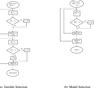
Set R, A, C to and V=X V Mˆ0j: 0 0 ˆj M Yes j R No Repeat J=1,…,d, V={X,Z} X Mˆ0j: 1 0 ˆ j M Yes C j A j No Repeat J✁R Output C and A
(a) Variable Selection
Use C , A and R. Set Ij= , ✁j✂R V=X V Mi j: ˆ() 1 2 ) ( 1 ˆi j M Yes j I i No Repeat i✂R, i Output Ij Repeat j✂R, V={X,Z(i)} (b) Model Selection
Figure 2: Flow-chart for the GRID procedure. Note thatX stands for Uniform random variables whileZ is the set of transformed random variables using (18). In particular, in figure (d), there isZ(i)which denotes the set of random variablesZ except the covariate i
which is Uniform, as described in the algorithm.
A. Proofs
In general, in the proofs of the LLE’s properties we follow the classic approach used in Lu (1996) and Ruppert & Wand (1994), a part from three substantial differences. The first is that here the bandwidths do not tend to zero for n → ∞ (see assumption A1). This implies that we must bound all the terms of the Taylor expansion with respect tom(x), given that the size of the interval around the pointx does not vanish with n → ∞. For the same reason, we must also bound the terms of the Taylor expansion with respect tofX(x),
the density function. To this aim, in Proposition 1 we consider assumptionA4, so that the Taylor expansion is exact with respect tofX. Then we relax assumptionA4 in Theorem
2. Finally, we want to analyze carefully the influences of the bandwidths associated to the different covariates on the bias ofβ(x; H). As a consequence, we will partition all theˆ involved matrices along the index sets{C, Ac, Au, U }.
Proof of Proposition 1:The conditional bias of the LLE is given by
E(β(x; H)|Xˆ 1, . . . , Xn) − β(x) = (ΓTW Γ)−1ΓTW (M − Γβ(x))
whereM = (m(X1), . . . , m(Xn))T andβ(x) = (m(x), DTm(x))T. Note that, givenut =
H−1(X
t− x), we have
n−1ΓTW Γ = diag(1, H)Sndiag(1, H) (27)
with Sn = 1 n n ∑ t=1 ( 1 uTt ut utuTt ) |H|−1K(ut) Rn = 1 n n ∑ t=1 ( 1 ut ) [m(Xt) − m(x) − DTm(x)Hut] |H|−1K(ut),
so the bias can be simply written as
E(β(x; H)|Xˆ 1, . . . , Xn) − β(x) = diag(1, H−1)S−1n Rn. (29)
ForSn, using Taylor’s expansion and assumptionA4, we have
Sn = ∫ ( 1 uT u uuT ) K(u)fX(x + Hu)du + Op(n−1/2) = fX(x) ∫ ( 1 uT u uuT ) K(u)du + ∫ ( 1 uT u uuT ) [DT f(x)Hu] K(u)du + Op(n−1/2) = ( 1 0 0 µ2Id ) + Op(n−1/2). (30)
For the analysis ofRn, we need to introduce some further notation. Given assumption
A3, let define the vth-order differential Dv
m(x; y) as Dvm(x, y) = ∑ i1,...,id v! i1! × . . . × id! ∂vm(x) ∂xi1 1 . . . ∂xidd yi1 1 × . . . × y id d, (31)
where the summation is over all distinct nonnegative integers i1, . . . , id such that i1 +
. . . + id = v. Using the Taylor’s expansion to approximate the function m(Xt), and the
assumptionA4, we can write Rn = 1 n n ∑ t=1 ( 1 ut ) [ 1 2!D 2 m(x, Hut) + 1 3!D 3 m(x, Hut) ] |H|−1K(ut) + R∗n = ∫ ( 1 u ) [ 1 2!D 2 m(x, Hu) + 1 3!D 3 m(x, Hu) ] K(u)fX(x + Hu)du + R∗n + Op(n−1/2) = ∫ ( 1 u ) [ 1 2!D 2 m(x, Hu) + 1 3!D 3 m(x, Hu) ] K(u)du + R∗n+ Op(n−1/2),
whereRn∗ represents the residual term, which depends on the higher order derivatives of the functionm(x). This element will be discussed later. Now remember that the odd-order moments of the kernel product are null, so some of the terms in thev-th order differentials cancel. We have Rn = ∫ ( 1 2!Dm2(x, Hu) 1 3!uD3m(x, Hu) ) K(u)du = ( γ1 γ2 ) + R∗n+ Op(n−1/2) (32)
whereγ1is a scalar, whileγ2is ad-dimensional vector. Solving the integrals and applying
the properties of the kernel we have γ1 = ∫ 1 2D 2 m(x, Hu)K(u)du = 1 2 d ∑ i=1 d ∑ j=1 ∂2m(x) ∂xi∂xj hihj ∫ uiujK(u)du = 1 2µ2 d ∑ i=1 ∂2m(x) ∂xi∂xi h2i = 1 2µ2tr{HHm(x)H}.
The componentγ2is a vector of lengthd. Its element of position r is
γ(r)2 = ∫ 1 6urD 3 m(x, Hu)K(u)du = ∑ i1,...,id hi1 1 · · · h id d i1! × . . . × id! ∂3m(x) ∂xi1 1 · · · ∂xidd ∫ ui1 1 · · · uirr+1· · · uiddK(u)du = ∑ s̸=r 1 2µ 2 2 ∂3m(x) ∂xr∂x2s hrh2s+ 1 6µ4 ∂3m(x) ∂x3 r h3r ,
while the whole vectorγ2is equal to
γ2 = 1 2µ 2 2 [ HGm(x)H2+ ( µ4 3µ2 2 − 1 ) diag{HGm(x)H2} ] 1.
concerning the residual termR∗n, using the assumptionA3 and remembering the (31), we can define δ(Dmv, HCv) ≤ ∑ i1,...,ik v! i1! · · · ik! sup x∈[0,1]d ∂vm(x) ∂xi1 1 . . . ∂x ik k hi1 1 × . . . × h ik k < ∞,
where the sum is taken for all the combination of indexesi1 + . . . + ik = v. Note that
δ(Dvm, HC) depends on the derivatives of total order v, which are bounded given
assump-tionA3. Moreover, it depends only on the bandwidths in HC. Then
R∗n= ( δ(D4 m, HC4) δ(Dm5, HC5) ) . Combining the (29), (30) and (32), we obtain
E(β(x; H)|Xˆ 1, . . . , Xn) − β(x) = diag{1, H−1}Sn−1Rn ≈ ( 1 0 0 µ12H−1 ) ( γ1 γ2 ) = 1 2µ2 ( tr(HHmH) Gm(x)H21+ ( µ4 3µ2 2 − 1 ) diag{Gm(x)H2}1 ) . (33)
Then we can further detail these expressions remembering the (6) and (7), and noting that ∀v, w HvHm(x)Hw = HCvHCm(x)HCw HCvHCAc m (x)HAwc 0 0 Hv AcH AcC m (x)HCw HAvcH Ac m(x)HAwc 0 0 0 0 HAvuHAu m (x)HAwu 0 0 0 0 0
HvGm(x)Hw = HCvGCm(x)Hw C 0 0 0 HAvcGAcC m (x)HCw 0 0 0 0 0 0 0 0 0 0 0 .
After some algebra, we have the result of the Proposition. ✷
Proof of Theorem 1:
It is sufficient to use the results shown in Proposition 1 w.r.t. the estimators ˙M0j and ˙M1j
defined in (15). Remembering the (27) and (28), we can write E(M (x; H)|X1, . . . , Xn) − β(x) = 1 ndiag(1, H −2)ΓTW M − β(x) = 1 ndiag(1, H −2)ΓTW (M − Γβ(x)) + 1 ndiag(1, H −2)ΓTW Γβ(x) − β(x)
= diag(1, H−1)Rn+[diag(1, H−1)Sndiag(1, H) − Id+1] β(x).
Now, using assumptionA4 and the results of Proposition 1, the bias of the estimator (15) is E(M (x; H)) − β(x) = ( bm(x; HC) µ2BD(x; HC) ) + ( 0 0 0 (µ2− 1)Id ) β(x). (34) So we obtain E (M0(x; H)) − m(x) = bm(x; HC)
where the estimatorM0(x; H) is defined in (13) and bm(x; HC) is the bias of LLE as in
Proposition (1). Taking the derivative w.r.t.hj, at both sides, we have
θm0j = E(M˙0j
)
= ∂
∂hj
bm(x; HC).
Sincebm(x; HC) depends on the bandwidths of the covariates in C, the first part of theorem
is shown. The detailed expressions of the expected derivativesθm 0j are θ0jm = { hjµ2∂ 2m(x) ∂2x j + δ(D 4 mj; H 4 C) ifj ∈ C 0 otherwise . (35)
Note thatδ(Dm4j; HC4) depends on the partial derivatives of order 4 involving the j-th co-variate, wherej ∈ C, which are bounded given assumption A3. So, it is equal to zero when ∂2m(x)/∂x2j = 0.
Now we consider the estimatorM1(x; H) in (13). Using again the (34) and the same
arguments as in the proof of Proposition (1), we have
E(M1(i)(x; H))− D(i)m(x) = µ2BD(i)(x; HC) + (µ2− 1)D(i)m(x)
where(i) stands for the component of position (i) in the vectors M1(x; H), Dm(x) and
BD(x; HC), i = 1 . . . , d. The quantity BD(x; HC) is defined in Proposition (1) and µ2
is the second moment of the KernelK. As before, taking the derivative w.r.t. hj, at both
sides, it follows
θmij = E(M˙1j(i))= ∂ ∂hj
Using (9) in Proposition (1) and remembering the (7), we know that∂h∂
jB
(i)
D (x; HC) ̸= 0
if and only ifi ∈ Ij andj ∈ C. Note that, for i ̸= j, Ij stands for set of covariates (linear
or nonlinear) which are mixed with the covariatej. The formula of the expected derivativesθijmare
θmij = { hjµ22∂ 3 m(x) ∂xi∂x2j + δ(D5 mij; H 5 C) ifi ∈ Ij, j ∈ C 0 otherwise . (36)
It can be shown thatδ(Dm5ij; HC5) includes the partial derivatives of order 5 involving both thei-th and j-th covariates. They are bounded given the assumption A3, and they are all
equal to zero when∂3m(x)/∂xi∂x2j = 0. ✷
Proof of Theorem 2: The key aspect of this proof is to show that the higher order terms of the Taylor expansion ofRn do not compromise the results of our procedure. In fact,
when A4 is not assumed, the derivatives of the density function fX are different from
zero, introducing further components in the Taylor expansion of Rn. Moreover, given
assumptionA1, such higher order terms may not vanish, contrary to what happens in the classic framework of local linear estimators, where the bandwidths tend to zero forn → ∞. In particular, the transformation Zt = φ(Xt) defined in (18) applied to the uniform
covariates Xt implies that the marginal density of each transformed covariate is linear,
being equal to
fZ(zi) = 2zi, i ∈ Au∪ U.
Because of the linearity, the gradient and the Hessian matrix of the density functionfZ(z)
are the following
Df(z) = 0 DAc f DAu f DU f Hf(z) = 0 0 0 0 0 HAc f H AcAu f H AcU f 0 HAuAc f H Au f H AuU f 0 HU Ac f H U Au f HUf , (37)
with the diagonal of Hf equal to zero. This implies that we need to consider the Taylor
expansion ofRnw.r.t. the derivatives offzup to order 4.
Now remember that, using the transformed variables Zt = φ(Xt) defined in (18), the
auxiliary regression function becomes
g(z) = g1(xC, zAc) + g2(zAc, zAu).
Therefore, given that the aim here is to identify the covariates inA = Ac ∪ Au, we can
focus on functiong2. This is further justified by the structure of Df(z) and Hf(z) shown
in (37). So, without loss of generality, we can usez = (zAc, zAu, zU) of d − k dimension.
The gradient and the Hessian matrix of functiong become Dg(z) = DAc g DAu g 0 Hg(z) = HAc g HAgcAu 0 HAuAc g HAgu 0 0 0 0 (38)
where the submatrices have changed compared with the first regression (in particular, note that HAc
g and HAguhave not a zero diagonal). Moreover, the matrix Gg(z) becomes
Gg(z) = GAc g GAgcAu 0 GAuAc g GAgu 0 0 0 0 , (39)
where the submatrices are defined as usual. In particular, note that GAc
g and GAgu are full
matrices with zero diagonal, as a consequence of theφ-tranformation of the covariates in A. Moreover we define with HZ,ΓZ,WZ andMZthe corresponding quantities w.r.t. H,
Γ, W and M using z whose dimension is d − k. Finally, let DZf and HZf be the same quantities as in (37) without the zeros. So that DZf is a vector of dimensiond − k and HZf is a matrix withd − k rows and d − k columns.
Using again the (27) and (28), we can write E(M (z; HZ)|Z1, . . . , Zn) − β(z)
= 1
ndiag(1, H
−2
Z )ΓZTWZMZ− β(z)
= diag(1, HZ−1)Rn+[diag(1, HZ−1)Sndiag(1, HZ) − Id+1−k] β(z),
but now we have to consider the higher order terms ofSnandRninduced byfZ.
Let us consider the vectorRnin the (32) with the additional nonzero terms of the Taylor
expansion w.r.t. fZ, using the assumptionsA1 − A4 and the transformed covariates. We
have E(Rn) = fZ(z) ∫ ( 1 2!Dg2(z, HZu) 1 3!uDg3(z, HZu) ) K(u)du + ∫ ( 1 3!Dg3(z, HZu)[(DZf(z))THZu] 1 2!uDg2(z, HZu)[(DZf(z))THZu] ) K(u)du + + ∫ ( 1 2!Dg2(z, HZu)[12uTHZHZf(z)HZu] 1 3!uD3g(z, HZu)[12uTHZHZf(z)HZu] ) K(u)du + ∫ ( 1 2!Dg2(z, HZu)[4!1D4f(z, HZu)] 1 3!uD3g(z, HZu)[4!1D4f(z, HZu)] ) K(u)du = R0+ R1+ R2+ R3,
where the four terms are equal to R0 = 1 2µ2fZ(z) ( tr (HZHgHZ) µ2[HZGgHZ2] 1 ) R1 = 1 2µ 2 2 ( (DZf)T [H2 ZGgHZ2] 1 [ 2HZHgHZ2 + HZtr (HZHgHZ) + ( µ4 µ2 2 − 3)diag(HZHgHZ2) ] DZ f ) R2 = 1 2µ2 µ2tr ( HZ fHZ2HgHZ2 ) µ22HZHZfHZ2GgHZ21+ (µ4− µ22) diag ( HZHZfHZ2GgHZ2 ) 1+ HZJg R3 = µ42 ( 0 HZLg ) , and Jgand Lgare vectors whosei-th element is equal to
J(i)g = 3µ22∑ s̸=i ∑ j̸={s,i} ∂2f Z(z) ∂zs∂zj h2s ∂ 3g(z) ∂zi∂zs∂zj h2j L(i)g = ∑ j̸=i ∑ s̸={j,i} ∑ u̸={j,s,i} ∂3g(z) ∂zj∂zs∂zu ∂4f Z(z) ∂zi∂zj∂zs∂zu h2jh2sh2u.
Note that the vector R2 has been derived exploiting the simple structure of HZf and Gg
(both with zero diagonal). For simplicity, we do not consider here the residual termR∗n, which can be analyzed following the same arguments as in Proposition 1.
ForSn, using Taylor’s expansion and assumptionsA1 − A4 with the transformed
covari-atesZ, we have E(Sn) = ∫ ( 1 uT u uuT ) K(u)fZ(z + HZu)du = fZ(z) ( 1 0 0 µ2Id−k ) + ( 0 µ2(DZf)THZ µ2HZDZf 0 ) + ( 0 0 0 µ2HZHZfHZ ) = ( fZ(z) µ2(DZf)THZ µ2HZDZf fZ(z)µ2Id−k+ µ2HZHZfHZ ) .
Note, again, that we have derived the previous result usingtr(HZHZfHZ) = 0, given the
linearity offZ.
The bias of the estimator (15), using the transformed covariates, becomes
E(M (z; HZ)) − β(z) = diag(1, HZ−1)(R0+ R1+ R2+ R3) (40) + [diag(1, H−1 Z ) E(Sn) diag(1, HZ) − Id+1−k] β(z), where diag((1, HZ−1))R0 = 1 2µ2fZ(z) ( tr (HZHgHZ) µ2[GgHZ2] 1 ) diag((1, HZ−1))R1 = 1 2µ 2 2 ( (DZf)T [H2 ZGgHZ2] 1 [ 2HgHZ2 + tr (HZHgHZ) Id−k+ ( µ4 µ2 2 − 3 ) diag(HgH2 Z )] DZf ) diag((1, HZ−1))R2 = 1 2µ2 µ2tr ( HZ fHZ2HgHZ2 ) µ22HZfHZ2GgHZ21+ (µ4− µ2 2) diag ( HZfHZ2GgHZ2)1+ Jg diag((1, HZ−1))R3 = µ42 ( 0 Lg ) and [diag(1, H−1 Z ) E(Sn) diag(1, HZ) − Id+1−k] β(z) = ( [fZ(z) − 1]g2(z) + µ2(DZf)THZDg µ2HZDZfg2(z) + [µ2fZ(z) − 1]Dg+ µ2HZHZfHZDg ) .
Now, the first part of the theorem, in the (19), can be easily shown observing the first component of each vector. Note that the bandwidth matrixHZ appears always multiplied
by Dg(z), Hg(z) or Gg(z). So, given v and w, we have
HZvHg(z)HZw = HAv cH Ac g (z)HAwc H v AcH AcAu g (z)HAwc 0 HAvuAcHAc g (z)HAwc H v AuH Au g (z)HAwu 0 0 0 0 = δ(HAc, HAu) HZvGg(z)HZw = δ(HA c, HAu) HZDg(z) = δ(HAc, HAu).
Therefore, we obtain
E (M0(z; HZ)) − g2(z) = δ(HAc, HAu) + [fZ(z) − 1]g2(z)]
where the estimator M0(z; HZ) is defined in (13) and uses the transformed covariates
Z(j), j ∈ A. Taking the derivative w.r.t. hj, at both sides, we have
θg0j = E (∂M0(z; HZ)/∂hj) = 0 ∀j /∈ A.
In oder to prove the second part of the theorem, in the (20), we must consider the second element of each vector in the (40). Following the same arguments as before, it can be shown that
E (M1(z; HZ)) − Dg(z) = δ(HAc, HAu) + [µ2fZ(z) − 1]Dg(z) + µ2HZD
Z fg2(z)
which implies that
θgij = E(∂M1(i)(z; HZ)/∂hj
)
= 0 ∀i ∈ Ξ, j ∈ U i ̸= j. (41) Anyway, we need to analyzeθijg fori ̸= j and j ∈ A, given that these values can be used to identify the mixed effect terms. So, we derive the exact formula ofθgij, fori ̸= j, equal to
θgij = µ2fZ(z)hj [ µ2 ∂3g2(z) ∂zi∂zj2 + 2µ2 ∂2g2(z) ∂zi∂zj ∂ log fZ(z) ∂zj ] + (42) + 6µ42hj ∑ s̸={i,j} ∂3g2(z) ∂zs∂zi∂zj ∂2fZ(z) ∂zs∂zj + µ2hj [ (µ4− µ22)h2i ∂3g2(z) ∂zj∂zi2 ∂2fZ(z) ∂zi∂zj ] + + µ2hj ∂2g2(z) ∂zj∂zj ∂fZ(z) ∂zi + µ22∑ s̸=i ∂3g2(z) ∂zs∂z2j ∂2fZ(z) ∂zi∂zs h2s+∂g2(z) ∂zj ∂2fZ(z) ∂zi∂zj + + 2µ42hj ∑ s̸={j,i} ∑ u̸={j,s,i} ∂3g2(z) ∂zj∂zs∂zu ∂4fZ(z) ∂zi∂zj∂zs∂zu h2sh2u.
We can see from the previous formula that θgij is different from zero if there are mixed effects between the two covariatesZ(i) andZ(j), that is when i ∈ Ij. Anyway, it can be
different from zero also wheni /∈ Ij, given that there are the terms in the third and fourth rows of the previous formula which depend on the partial derivatives ofg2w.r.t. covariates
different from(i, j). In order to make this as a one to one relation, it is necessary to force to zero the third and fourth rows of the formula. This can be done considering a uniform density forZ(i), because in such a case all the terms in the third and fourth rows (but also the term in the second row) would be canceled by the derivative∂fZ(z)/∂zi, equal to zero.
Therefore, we suggest not to transform thei-th covariate in the auxiliary regression. This proves the third part of the theorem, in the (21).
The formula of the expected derivativeθ∗ij, fori ̸= j, is
θij∗ = µ22fZ(z)hj [ ∂3g 2(z) ∂zi∂z2j + 2∂ 2g 2(z) ∂zi∂zj ∂ log fZ(z) ∂zj ] + 6µ42hj ∑ s̸=i,j ∂3g 2(z) ∂zs∂zi∂zj ∂2f Z(z) ∂zs∂zj . (43) ✷
Proof of Proposition 2: First, we have n E(V ar( ˙M0j|X1, . . . , Xn) ) = σ2E [ ∂ ∂hj 1 |H|2K 2(H−1(X − x)) ] .
By assumptions (A1)-(A4) we can change the mean operator w.r.t. the derivative operator. Therefore, n E(V ar( ˙M0j|X1, . . . , Xn) ) = σ2 [ ∂ ∂hj ( |H|−1/2) ]2 E[|H|−1K2(H−1(X − x))] .
Changing the variableu = H−1(X − x) we have the result in (i). For point (ii), we have
n E(V ar( ˙M1j|X1, . . . , Xn) ) = σ2E [ ∂ ∂hj ( H−2(X − x) 1 |H|2K 2(H−1(X − x)) (X − x)TH−2 )] .
Changing the variableu = H−1(X − x) and using the same arguments as in point (i), it follows n E(V ar( ˙M1j|X1, . . . , Xn) ) = σ2 [ ∂ ∂hj ( H−1|H|−1/2) ]2 E(uuTK2(u)) = σ2ν2ν0d−1 4|H|h2 j H−2Ij. ✷ References
Bertin K. and Lecue G. (2008) Selection of variables and dimension reduction in high-dimensional non-parametric regression. Electronic Journal of Statistics, 2, 1224–1241. Chen X.S., Peng L. and Qin Y.L. (2009) Effects of data dimension on empirical likelihood.
Biometrika, 96, 711–722.
DiCiccio T., Hall P. and Romano J. (1991) Empirical Likelihood is Bartlett-Correctable.
The Annals of Statistics, 19, 1053–1061.
Hall P. (1992) The Bootstrap and Edgeworth Expansion. Springer, New York.
Hall P., La Scala B. (1990) Methodology and Algorithms of Empirical Likelihood.
Inter-national Statistical Review, 58, 109–127.
Lafferty J., Wasserman L. (2008) RODEO: sparse, greedy nonparametric regression. The
Annals of Statistics, 36, 28–63.
Lahiri S.N., Mukhopadhyay S. (2012) Supplement to "‘A penalized empirical likelihood method in high dimensions"’. DOI:10.1214/12-AOS1040SUPP .
Lahiri S.N., Mukhopadhyay S. (2012) A penalized empirical likelihood method in high dimensions. The Annals of Statistics, 40, 2511–2540.
Lu Z.Q. (1996) Multivariate locally weighted polynomial fitting and partial derivative estimation. Journal of Multivariate Analysis, 59, 187–205.
Masry E. (1996) Multivariate local polynomial regression for time series: uniform strong consistency and rates. Journal of Time Series Analysis, 17, 571–599.
Owen A. (1990) Empirical Likelihood Ratio Confidence Regions. The Annals of Statistics, 18, 90–120.
Radchenko P., James G.M. (2010) Variable selection using adaptive nonlinear interaction structures in high dimensions. Journal of American Statistical Association, 105, 1541– 1553.
Storlie C.B., Bondell H.D., Reich B.J., Zhang H.H. (2011) Surface estimation, variable selection, and the nonparametric oracle property. Statistica Sinica, 21, 679–705. Ruppert D., Wand P. (1994) Multivariate locally weighted least squares regression. Annals
of Statistics, 22, 1346–1370.
Zhang H.H., Cheng G., Liu Y. (2011) Linear or nonlinear? Automatic structure discovery for partially linear models. Journal of American Statistical Association, 106, 1099–1112.