Dipartimento Di3A
Sezione Meccanica e Meccanizzazione
CLAUDIA AGLIECO
First results on the assessment of impact damage of vegetables by means of the FEM approach
TESI PER IL CONSEGUIMENTO DEL TITOLO DI
DOTTORE DI RICERCA
Tutor: Chiar.mo Prof. Emanuele Cerruto
Coordinatore: Chiar.ma Prof.ssa Simona Consoli
Dottorato di ricerca in Ingegneria Agraria - XXVI ciclo ANNO2014
tranne quella che sono (cit. A.C.)
At this successful completion of this doctoral research work I naturally would like to take this moment to pause, reflect and acknowledge all those people who have in one way or another been very helpful throughout my period of stay and subsequent production of this thesis.
First of all I would like to extend my heartfelt gratitude to my professor, Prof. Emanuele Cerruto, for taking a chance with me; for the enormous support (technical and moral) and encouragement; for his kindness and for the inexplicable and overwhelming confidence he expended on me. The amount of knowledge and academic/scientific maturity I was able to gain under him is simply beyond any measure. For these I am, and will always be, truly grateful.
My sincere gratitude also goes to the Institut für Agrartechnik, Potsdam-Bornim (ATB) for the good opportunity to use their prestigious laboratory for my research and to work in a international and stimulating working environment. In particular I would like to thank the Prof. Dr. Ing. Klaus-Günter Gottschalk who, in addition to his kindness in accepting to be my co-professor, has also helped facilitate during my stay in Potsdam-Bornim. I will always appreciate the cheerful words of encouragement and advice he has always offered at every opportunity.
Last, but not least, I wish to thank my family for the constant support and love.
Mechanical harvest and post-harvest handling induce numerous mechanical impacts on vegetables. These impacts may cause damage such as black-spot bruise, resulting in severe economic losses.
Impact forces and accelerations arising from collisions, are among the main indices taken into account when studying the damage of fruit and veg-etables during post-harvest activities. A miniaturised Acceleration Measuring Unit (AMU) has been recently developed at the Institut für Agrartechnik, Potsdam-Bornim (ATB): when implanted into a real product like a potato tuber, it is able to measure the accelerations at the centre of the fruit deriving from a impact.
This PhD Thesis represents a first contribution on the study of mechanical impacts of vegetables (potato tubers), arising from mechanical harvest and post-harvest handling, by means of simulations based on the Finite Element Method (FEM) approach. Simulations were developed by using the Linux dis-tributionCAElinux2011, that contains several technical-engineering software, among which stand out Salome-Meca and Code-Aster. Salome-Meca was used for modelling, meshing and post-processing activities, while Code-Aster was used for processing models.
The work has been developed in collaboration with the Institut für Agrar-technik, Potsdam-Bornim (ATB), Germany, where they were conducted lab-oratory tests (drop tests to measure impact forces and texture analyses to measure modulus of Young) with two spherical artificial fruits.
After the development of several preliminary simple models to gain fa-miliarity with the computational software Salome-Meca and Code-Aster and to acquire an acceptable agreement between simulated and experimental
of the fruit, density and modulus of Young of the material, on the impact indices (maximum impact force and maximum acceleration at the centre of the fruit). Simulated material parameters were chosen to approach potato tubers properties.
All the factors examined (drop height, sphere diameter, modulus of Young and density of the material, mass of the fruit) affected the maximum impact force and the maximum acceleration at the centre of the sphere. Their increase always caused an increase in the maximum impact force, whereas the maxi-mum acceleration at the centre of the sphere decreased vs sphere diameter, material density and mass, and increased vs drop height and modulus of Young. The decreasing trends are due to the cushioning effect produced by the sphere material itself.
Moreover, the maximum impact forces reported in the experimental re-sults by Geyer et al. (2009), referring to drop tests of potato tubers onto steel plates, are in good agreement with the values of impact forces provided by the simulations. Instead, simulations provided acceleration values about twice as many those measured in the experimental results with the AMU device. This difference could be due to the implantation system of the AMU inside the tuber. In fact, comparing the measured impact force and the force computed by means the second law of Newton(F = m·a), Geyer et al. in the cited work report that the computed force was approximately half the measured one, meaning an under-estimation of the acceleration provided by the AMU.
Ultimately, the concordance between measured and simulated impact forces confirmed the validity of FEM approach, although the limitations owing to the simplicity of the model developed in this work.
Acknowledgements 3
Abstract 4
List of Figures 8
List of Tables 12
Foreword 13
1 Post harvest of fruit and vegetables 15
1.1 General aspects . . . 15
1.2 Impact damage on potato tubers . . . 16
1.3 Relationship between damage and methods of harvesting . . 17
1.4 Potato shaped instrumented devices . . . 18
2 Basic concepts on FEM 22 2.1 General aspects . . . 22
2.2 Brief history of the Finite Element Method . . . 22
2.3 Basics on the Finite Element Method . . . 24
2.4 Computational modelling using FEM . . . 25
2.5 Modelling of the geometry . . . 26
2.6 Meshing . . . 26
2.7 Property of the material . . . 27
3 Materials and Methods 29
3.1 General aspects . . . 29
3.2 The Salome-Meca software . . . 30
3.3 The Code-Aster software . . . 31
3.4 FEM analysis . . . 32
3.5 Preliminary tests . . . 33
3.6 The experimental activity at ATB . . . 34
3.6.1 Measurement of the modulus of Young . . . 35
3.6.2 Drop tests with artificial fruits . . . 38
3.7 Drop test simulations . . . 40
4 Results and Discussion 42 4.1 General aspects . . . 42 4.2 Preliminary tests . . . 42 4.2.1 Study 1 . . . 42 4.2.2 Study 2 . . . 51 4.2.3 Study 3 . . . 58 4.2.4 Study 4 . . . 63 4.2.5 Study 5 . . . 69 4.2.6 Study 6 . . . 80
4.3 Measurement of the modulus of Young . . . 81
4.4 Drop tests . . . 83
4.5 Drop test simulation . . . 85
4.5.1 Preliminary simulations . . . 85
4.5.2 Model building . . . 87
4.5.3 Effect of drop height . . . 97
4.5.4 Effect of modulus of Young . . . 101
4.5.5 Effect of diameter . . . 105
4.5.6 Effect of density . . . 108
4.5.7 Effect of mass . . . 109
Conclusions 114
1.1 Instrumented Sphere IS 100. . . 19
1.2 Instrumented Sphere PMS 60 developed at ATB. . . 19
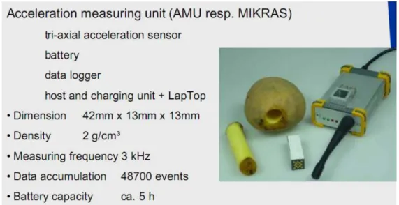
1.3 Specification and view of miniaturised acceleration measuring unit (AMU) and its implantation in potato tuber. . . 21
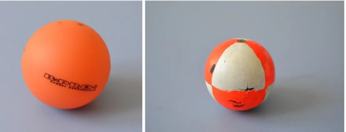
3.1 The two artificial fruits used for the drop tests: BALL 1 (left) and BALL 2 (right). . . 35
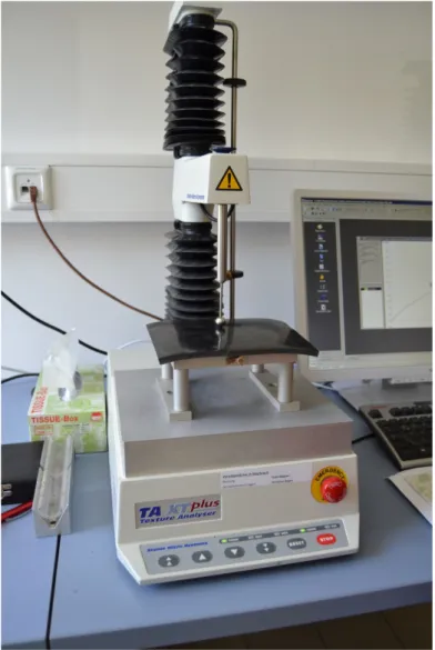
3.2 The texture analyser for calculating the modulus of Young. . . 36
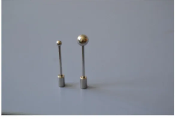
3.3 Spherical probes for measuring the modulus of Young. . . 37
3.4 Positioning of the sphere for measuring the modulus of Young. 37 3.5 Hertz contact of two spheres. . . 37
3.6 Schematic view of the drop simulator. . . 39
3.7 The two impact materials: steel and PVC. . . 40
4.1 Normal stress. . . 43
4.2 Deformed shape. . . 50
4.3 Displacements of the Pressure face nodes. . . 50
4.4 Stress distribution along the box. . . 50
4.5 Deformed shape of the two boxes. . . 57
4.6 Deformed shape of the Box_2. . . 57
4.7 Displacements of the Pressure face nodes. . . 57
4.8 Stress distribution along the boxes. . . 58
4.9 Deformed shape of the sphere. . . 62
4.11 Stress distribution along a line on the upper face of the sensor
inside the sphere. . . 63
4.12 Displacement of the “Node 5” over the time. . . 69
4.13 Velocity of the “Node 5” over time. . . 69
4.14 Acceleration of the “Node 5” over time. . . 69
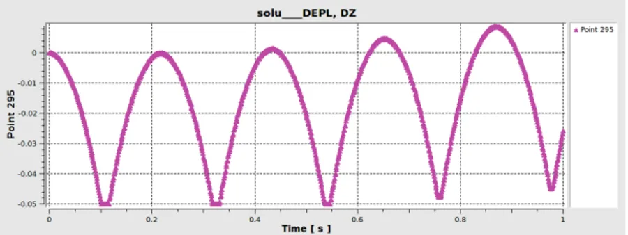
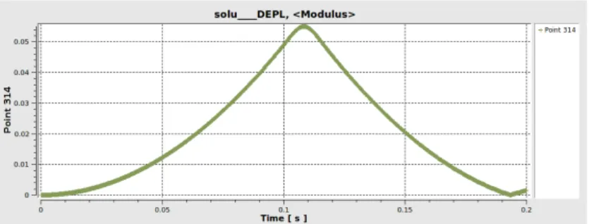
4.15 Displacement along the z-axis of the “Node 295” over the time. 79 4.16 Displacement along the z-axis of the “Node 314” over time. . . 79
4.17 Modulus of the displacement of the “Node 295” over time. . . 80
4.18 Modulus of the displacement of the “Node 314” over time. . . 80
4.19 Box-plots of the modulus of Young values at varying artificial fruits and probe diameters. . . 81
4.20 Example of file with force data. . . 83
4.21 Box-plots of the force values measured during the drop tests with the two artificial fruits. . . 84
4.22 Geometric model used for the drop tests. . . 85
4.23 Comparison between simulated and measured force in drop tests. . . 87
4.24 Geometric model used for drop tests after meshing. . . 91
4.25 Maximum impact force vs drop height at varying modulus of Young (MPa) and density (kg/m3) when the sphere diameter was 50 mm. . . 97
4.26 Maximum impact force vs drop height at varying modulus of Young (MPa) and density (kg/m3) when the sphere diameter was 65 mm. . . 98
4.27 Maximum impact force vs drop height at varying modulus of Young (MPa) and density (kg/m3) when the sphere diameter was 80 mm. . . 98
4.28 Maximum acceleration at the centre of the sphere vs drop height at varying modulus of Young (MPa) and density (kg/m3) when the sphere diameter was 50 mm. . . 99
4.29 Maximum acceleration at the centre of the sphere vs drop height at varying modulus of Young (MPa) and density (kg/m3) when the sphere diameter was 65 mm. . . 100
4.30 Maximum acceleration at the centre of the sphere vs drop height at varying modulus of Young (MPa) and density (kg/m3) when the sphere diameter was 80 mm. . . 100 4.31 Average impact force vs modulus of Young. . . 101 4.32 Maximum impact force vs modulus of Young at varying drop
height (cm) and density (kg/m3) when the sphere diameter was 50 mm. . . 102 4.33 Maximum impact force vs modulus of Young at varying drop
height (cm) and density (kg/m3) when the sphere diameter was 65 mm. . . 103 4.34 Maximum impact force vs modulus of Young at varying drop
height (cm) and density (kg/m3) when the sphere diameter was 80 mm. . . 103 4.35 Maximum acceleration at the centre of the sphere vs modulus
of Young at varying drop height (cm) and density (kg/m3) when the sphere diameter was 50 mm. . . 104 4.36 Maximum acceleration at the centre of the sphere vs modulus
of Young at varying drop height (cm) and density (kg/m3) when the sphere diameter was 65 mm. . . 104 4.37 Maximum acceleration at the centre of the sphere vs modulus
of Young at varying drop height (cm) and density (kg/m3) when the sphere diameter was 80 mm. . . 105 4.38 Maximum impact force vs sphere diameter at varying drop
height (cm) and density when the modulus of Young was 0.5 MPa. . . 106 4.39 Maximum impact force vs sphere diameter at varying drop
height (cm) and density when the modulus of Young was 3.5 MPa. . . 106 4.40 Maximum acceleration at the centre of the sphere vs sphere
diameter at varying drop height (cm) and density when the modulus of Young was 0.5 MPa. . . 107
4.41 Maximum acceleration at the centre of the sphere vs sphere diameter at varying drop height (cm) and density when the modulus of Young was 3.5 MPa. . . 107 4.42 Maximum impact force vs material density at varying drop
height and sphere diameter (mm) when the modulus of Young was 3.5 MPa. . . 108 4.43 Maximum acceleration at the centre of the sphere vs
mate-rial density at varying drop height and sphere diameter (mm) when the modulus of Young was 3.5 MPa. . . 109 4.44 Maximum impact force vs mass at varying drop height (cm),
assuming as parameter the modulus of Young. . . 110 4.45 Maximum impact force vs mass at varying modulus of Young
(MPa), assuming as parameter the drop height. . . 110 4.46 Maximum acceleration at the centre of the sphere vs mass at
varying drop height (cm), assuming as parameter the modulus of Young. . . 111 4.47 Maximum acceleration at the centre of the sphere vs mass at
varying modulus of Young (MPa), assuming as parameter the drop height. . . 112 4.48 Correlation between simulated and computed force. . . 113
1.1 Proportion of potato damage per handling stage to total damages. 18 3.1 Main features of the two artificial fruits. . . 34 4.1 Results of the analysis of variance on modulus of Young values. 82 4.2 Results of the analysis of variance on deformation values. . . . 82 4.3 Mean values of deformations and moduli of Young (E). . . 82 4.4 Mean values of impact force measured during the drop tests. . 85 4.5 Parameters used for the drop tests. . . 86
This PhD Thesis represents a first contribution on the study of mechanical impacts on vegetables (potato tubers) arising from mechanical harvest and post-harvest handling.
The impacts may cause damage such as black spot bruise, resulting in severe economic losses. Besides the direct effect of fruit bruising on vegetables quality, and, hence, the visual quality appreciation by the consumer, an important indirect effect can be identified as damaged tissue, a good avenue for entrance of decay organisms, which decrease the shelf-life of the fruit drastically.
A computer simulation technique, named Finite Element Method (FEM), was applied to get insight in the mechanical impact. FEM is essentially a numerical method to find approximate solution of problems in engineer-ing. FEM is best understood from its practical application, known as Finite Element Analysis (FEA).
Finite element analysis is the modelling of products and systems in a virtual environment, for the purpose of finding and solving potential (or existing) structural or performance issues. FEA is used by engineers and scientists to mathematically model and numerically solve very complex struc-tural, fluid, and multi-physics problems. FEA software can be utilised in a wide range of industries, but it is most commonly used in the aeronautical, biomechanical and automotive industries.
The assessment of impact damage of vegetables by means of FEM is the aim of this Thesis, that has been developed in collaboration with the Institut für Agrartechnik, Potsdam-Bornim (ATB), Germany. I spent a part of my doctorate in Potsdam under the supervision of the Prof. Dr. Ing. Klaus-Günter
Gottschalk, Senior scientist of Postharvest Technology Department.
The Thesis is structured in a first part relating to theoretical notions about the post-harvest and the FEM approach, whereas the latter end is focused on the experimental activity.
The first chapter focuses on the impact damage of potato tubers and on the development of potato-shaped instrumented devices to locate bruising risk zones and to prevent quality losses of commodity.
The second chapter presents some basic concept of FEM: what is FEM and the main steps required to develop a computational model using the FEM approach.
The third chapter is dedicated to the materials and methods of the research. In particular, the early paragraphs present the software used to develop the FEA and the preliminary studies developed to gain familiarity with it, while the remainder paragraphs show the experimental activity, dealing with the assessing, by means of drop test simulations of spherical pseudo-fruits, of the effects of material properties (density, size, modulus of elasticity, mass) and drop height on some impact indexes (impact force and acceleration).
Post harvest of fruit and vegetables
1.1
General aspects
All fruit and vegetable products are subject to different stress levels both during harvest and during subsequent post-harvest processing. This stress sometimes becomes so great to cause damage to the produce, compromising its preservability (Lewis et al., 2007). Even low levels of damage can bring about considerable economic loss, jeopardizing storage of the produce due to the risk of rotting that can then extend to entire batches.
It therefore becomes important, above all, to measure the intensity of the impacts to the produce during harvest and post-harvest activities and subsequently to correlate it with the probability of damage to the produce itself (Hyde et al., 1992; Tennes et al., 1991; Ito et al., 1994; Blandini et al., 2002; Blandini et al., 2003).
It should also be considered that each product has its own level of resis-tance to external stresses, which depend on the level of ripeness and other intrinsic factors, so that it appears fundamental to evaluate the stress thresh-old under which no damage is produced, in order to obtain products of high quality and extended storage capacity.
1.2
Impact damage on potato tubers
Potato (Solanum tuberosum) is one of the mankind’s most valuable food crops. It is grown in more countries than any other crop with the exception of maize, and ranks fourth in volume of production. Limitations to its productivity are, therefore, of widespread economic interest.
The potato tuber is largely parenchymatous, lacking specialised secondary thickened tissues. As a result, tubers are susceptible to various forms of dam-age during commercial production, including external and internal defects. Internal damage, resulting from the effects of impacts on tubers during har-vesting operations alone, may cause losses exceeding 20% (Storey and Davies, 1992).
Whilst it is a simple matter to grade out tubers showing external damage, internal damage is not visible until after peeling. The symptoms of internal damage may or may not include visible tissue fractures, and ensuing colour development of damaged areas may involve the formation of yellow, red, brown, blue, grey and black pigmentation to varying degrees (Burton, 1989; Gray and Hughes, 1978; Storey and Davies, 1992).
Damage sometimes includes the development of floury-white regions in clear contrast to the cream background of undamaged tissue. Where there is no visible fracture and colour development proceeds to a black end-product, the syndrome is usually referred to as internal bruising, though the terms “black spot” and “blue spot” are also common in the literature (Hiller et al.,
1985).
Common feature of the internal damage is that it almost certainly results from impact. This may seem obvious, but the fact that external damage has not occurred, suggests that tuber tissue responds differentially because of intrinsic differences in the biological properties of different layers and/or because it has been exposed to different stresses.
For example, damage from impact at higher energy levels is usually visible as fracture through all external layers, simply because external tissue has been insufficiently strong to withstand the incident stress. Once this stress has been concentrated into a crack in the outside layer, then damage proceeds
rapidly through deeper layers (McGarry et al., 1995).
For impacts below this level of energy, deformation and distribution of stress within the tissues create the potential for damage. Physical and biochemical properties of the tissue determine the internal response to the impact.
1.3
Relationship between damage and methods of
harvesting
Potatoes play a significant role in the human nutrition in many countries all over the world. An efficient crop production requires high mechanised processes in all stages. Therefore, potatoes are handled several times during harvesting, transport and storage. Each handling operation leads to me-chanical damage depending on the height of fall and the number of drops involved.
This damage causes substantial economic losses to the fresh market and the potato processing industry. One of the most serious defect problem is the occurrence of “black spots”. A lot of investigations took place in the recent years to examine the reason for formation of black spots and the susceptibility of the potato tubers to black spot development from mechanical impacts (Molema, 1999).
It was established that the black spot development depends, among others things, on physical, physiological and biochemical properties of the tuber. Other important influence parameters are genotype, development and envi-ronment (McGarry et al., 1996).
Although all the interrelations are now better understood, the reduction of mechanical stress is the best way to avoid black spots. In consideration of this fact, a gentle handling of potatoes from the harvest to the storage has to be achieved.
Currently, two methods of harvesting are widely used:
1. The harvested potatoes are passed via a discharge belt onto a transport vehicle which is driving alongside the harvester.
2. The potatoes are collected in a hopper on board the harvester. When the hopper is full, the content is transferred to the transport vehicle, either on the field or at the edge of the field.
At the storage hall the tubers are tipped out, separated of soil and stones as far as possible and brought into storage via a conveyor belt system. During each handling stage the potatoes are exposed to mechanical stress which leads to damage (Table 1.1).
Table 1.1: Proportion of potato damage per handling stage to total damages (Bouman, 1995).
Handling stage Damage (%)
Harvest 14.7
Transport and interim storage 0.5 Conveyor belt and stationary filler 1.5
Storage 20.8
Removal of potatoes 12.2
Loading lorry 14.2
Unloading lorry 3.0
Processing (sorting to packing) 33.1
The highest percentage of damage occurs during processing (33.1%), but farmers often cannot influence this damage. Important for the farmer is the question, how can be reduced the damage from harvest until the end of storage. In total, one-third of the damage occur from harvest until the end of the storage.
To avoid damage caused by handling, transport and storage, farmers are tending to fill the potatoes into storage boxes immediately after harvesting. Boxes are brought to the fields in transport vehicles and filled by the harvester.
1.4
Potato shaped instrumented devices
Potato tubers are often exposed to unnecessarily high mechanical loads at many steps in the production chain from harvesting to packaging (Bentini et
al., 2006). These mechanical impacts can cause various external and internal injuries in potatoes, particularly black spot bruise (Molema, 1999; Peters, 1996).
Although many efforts have been made to improve black spot bruising, the best approach is to eliminate or at least to reduce the risk of mechanical impacts during processing.
In a large number of studies the effects of actions influencing product quality during harvesting and subsequent processes are evaluated by using defined criteria. In order to reduce economic losses for growers and the potato industry due to mechanical damage, electronic spheres or potato-shaped instrumented devices are often used to measure handling impacts of tubers (Herold et al., 2001; Van Canneyt et al., 2003; Maly et al., 2005; Praeger et al., 2013; Opara & Pathare, 2014).
To characterise the most important sources of mechanical loads in the pro-duction chain, so-called artificial fruits such as IS 100 (Figure 1.1) (United State Department, Michigan Agricultural Experiment Station and Michigan State University, 1989, USA) (Zapp et al., 1990), PTR 100 (Bioteknisk Istitut, 1990, Denmark), PMS 60 (Figure 1.2) (Institut für Agrartechnik, Potsdam-Bornim (ATB), 1992, Germany) (Herold et al., 1996), PTR 200 (SM Enginnering Den-mark, 1999) and the “Smart Spud” (Sensor Wireless, 2000, Canada) (Bollen, 2006) have been available since several years.
Figure 1.1: Instrumented Sphere IS 100.
Figure 1.2: Instrumented Sphere PMS 60 developed at ATB.
These instrumented devices are sufficiently equipped and frequently ap-plied to locate those zones in the harvesting and processing chain that present a high level of risk of damage (Molema, 1999; Baheri, 1997). They consist of electronic impact measurement systems placed in a hard rubber or plastic body that simulates the real fruit. These instruments measure the actual mechanical impacts at different processing steps and can thus be helpful in identifying the potential risks of mechanical damage and in evaluating measures to reduce impact loads.
However, the damage predictive value of the earlier instruments IS 100, PTR 100 and PMS 60 has been frequently discussed in scientific literature: the information given by harvested and handled potatoes does not always corre-spond sufficiently with the information given by the instrumented devices. Among biological bruise susceptibility factors, natural variation in impact events, operating insufficiency of the devices for damage prediction purposes or difficult in data interpretation may cause this discrepancy (Leicher, 1992; Nerinckx and Verschoore, 1993).
The knowledge achieved so far by the instruments has not provided an important contribution to reducing the economic losses due to black spots in practice (Bollen et al., 2001; Bollen, 2006). Indeed, the limited practical use of instruments is mainly due to the considerable differences between real and artificial fruit, largely restricting the transferability of measured impact data to mechanical load onto real products. The IS 100 and the other devices are not able to truly simulate the biological and physical properties (shape, elasticity, surface proprieties) of potato tubers.
Recently, a new approach has been proposed to overcome these disadvan-tages of artificial fruits. Based on a miniaturized impact detecting system, a self-contained Acceleration Measuring Unit (AMU) has been developed at the ATB Leibniz-Institut für Agrartechnik, Potsdam-Bornim, small enough to be fitted into a real product without significant changes of the product’s properties (Figure 1.3). This AMU is suited to be integrated into a potato tuber and to record acceleration events acting on the tuber at many steps of the production chain.
Figure 1.3: Specification and view of miniaturised acceleration measuring unit (AMU) and its implantation in potato tuber (Praeger et al., 2013).
potato tuber based on the tuber’s actual physiological and physical properties. However, it is not known whether these properties affect the measuring characteristics of the AMU. Additionally, the technique of implanting the AMU (preparing the product, fitting and positioning the AMU) may influence the measuring data.
Basic concepts on FEM
2.1
General aspects
The Finite Element Method (FEM), sometimes referred to as Finite Element Analysis (FEA), is a computational technique used to obtain approximate solutions of problems in engineering.
The basic idea in the finite element method is to find the solution of a complicated problem by replacing it by a simpler one. Since the actual problem is replaced by a simpler one, in finding the solution we will be able to find only an approximate solution rather than the exact solution.
The existing mathematical tools will not be sufficient to find the exact solution of most of the practical problems. Thus, in the absence of any other convenient method to find even the approximate solution of a given problem, we have to prefer the finite element method.
Moreover, in the finite element method, it will often be possible to improve or refine the approximate solution by spending more computational effort.
2.2
Brief history of the Finite Element Method
The term finite element was first used by Clough in 1960 in the context of plane stress analysis and has been in common usage since that time.
During the decades of the 1960s and 1970s, the finite element method was extended to applications in plate bending, shell bending, pressure vessels,
and general three-dimensional problems in elastic structural analysis (Melosh, 1961; Melosh, 1963) as well as to fluid flow and heat transfer (Martin, 1968; Wilson and Nickell, 1966). Further extension of the method to large deflections and dynamic analysis also occurred during this time period (Turner et al., 1960; Archer, 1965). An excellent history of the finite element method and detailed bibliography is given by Noor (1991).
The mathematical roots of the finite element method, instead, dates back at least a half century. Approximate methods for solving differential equations using trial solutions are even older in origin. Lord Rayleigh (1870) and Ritz (1909) used trial functions to approximate solutions of differential equations. Galerkin (1915) used the same concept for solutions.
The drawback in the earlier approaches, compared to the modern finite element method, is that the trial functions must apply over the entire domain of the problem of concern. While the Galerkin method provides a very strong basis for the finite element method not until the 1940s, when Courant (1943) introduced the concept of piecewise-continuous functions in a sub-domain, did the finite element method have its real start.
In the late 1940s, aircraft engineers were dealing with the invention of the jet engine and the needs for more sophisticated analysis of airframe structures to withstand larger loads associated with higher speeds. These engineers collectively known the flexibility of the method, in which the unknowns are the forces and the knowns are the displacements (Hutton, 2004).
The finite element method, in its most often-used form, corresponds to the displacement method, in which the unknowns are system displacements in response to applied force systems. This application of simple finite ele-ments for the analysis of aircraft structure is considered as one of the key contributions in the development of the finite element method.
The digital computer provided a rapid means of performing the many calculations involved in the finite element analysis and made the method practically viable. Along with the development of high-speed digital com-puters, the application of the finite element method also progressed at a very impressive rate (Rao, 2004). The book by Przemieniecki (1968) presents the finite element method as applied to the solution of the stress analysis
prob-lems. Zienkiewcz and Cheung (1967) present the broad interpretation of the method and its applicability to any general filed problem.
2.3
Basics on the Finite Element Method
The Finite Element Method (FEM) has been developed into a key, indispens-able technology in modelling and simulating advanced engineering systems in various fields like housing, transportation, communications, and so on. In building such advanced engineering systems, engineers and designers go through a sophisticated process of modelling, simulation, visualization, analysis, designing, prototyping, testing, and lastly, fabrication. Note that much work is involved before the fabrication of the final product or system. This is to ensure the workability of the finished product, as well as for cost effectiveness.
FEM was first used to solve problems of stress analysis, and then has been applied to many other problems like thermal analysis, fluid flow analysis, piezoelectric analysis, and many others. In all the applications, the analyst seeks to determine the distribution of some field variable: in stress analysis it is the displacement field or the stress field; in the thermal analysis it is the temperature field or the heat flux; in fluid flow it is the stream function or the velocity potential function; and so on.
FEM is a numerical method seeking an approximated solution of the distribution of field variables in the problem domain that is difficult to obtain analytically (Liu and Quek, 2003). It is a way of getting a numerical solution to a specific problem. A Finite Element Analysis does not produce a formula as a solution nor does it solve a class of problems.
An unsophisticated description of FEM is that it involves cutting a struc-ture into several elements (pieces of the strucstruc-ture), describing the behaviour of each element in a simple way, then reconnecting elements at “nodes” as if nodes were drops of glue that hold elements together. This process re-sults in a set of simultaneous algebraic equations. In stress analysis these equations are equilibrium equation of the nodes. There are may be several hundred or several thousand of such equations, which means that computer implementation is mandatory (Cook, 1995).
There are numerous physical engineering problems in a particular system. As mentioned earlier, although FEM was initially used for stress analysis, many other physical problems can be solved. Mathematical models of FEM have been formulated for many physical phenomena in engineering systems. Common physical problems solved using the standard FEM include:
• mechanics for solids and structures; • heat transfer;
• fluid mechanics.
2.4
Computational modelling using FEM
The behaviour of a phenomenon in a system depends upon the geometry or domain of the system, the property of the material or medium, and the boundary, initial and loading conditions.
For an engineering system, the geometry or domain can be very com-plex. Further, the boundary and initial conditions can also be complicated. It is therefore, in general, very difficult to solve the governing differential equation via analytical means. In practice, most of the problems are solved using numerical methods. Among these, the methods of domain discretiza-tion championed by FEM are the most popular, due to its practicality and versatility.
The procedure of computational modelling using FEM broadly consists of four steps (Liu and Quek, 2003):
1. modelling of the geometry; 2. meshing;
3. specification of material properties;
2.5
Modelling of the geometry
Real structures, components or domains are in general very complex, and have to be reduced to a manageable geometry. Curved parts of the geom-etry and its boundary can be modelled using curves and curved surfaces. However, it should be noted that the geometry is eventually represented by a collection of elements, and the curves and curved surfaces are approximated by piecewise straight lines or flat surfaces, if linear elements are used.
Depending on the software used, there are many ways to create a proper geometry in the computer for the Finite Element (FE) mesh. Points can be created simply by keying in the coordinates. Lines and curves can be created by connecting the points or nodes. Surfaces can be created by connecting, rotating or translating the existing lines or curves; and solids can be created by connecting, rotating or translating the existing surfaces. Points, lines and curves, surfaces and solids can be translated, rotated or reflected to form new ones.
Graphic interfaces are often used to help in the creation and manipulation of the geometrical objects. There are numerous Computer Aided Design (CAD) software packages used for engineering design which can produce files containing the geometry of the designed engineering system. These files can usually be read in by modelling software packages, which can significantly save time when creating the geometry of the models.
However, in many cases, complex objects read directly from a CAD file may need to be modified and simplified before performing meshing or dis-cretisation. It may be worth mentioning that there are CAD packages which incorporate modelling and simulation packages, and these are useful for the rapid prototyping of new products.
2.6
Meshing
Meshing is performed to discretise the geometry created into small pieces called elements or cells.
very time consuming task to the analyst, and usually an experienced analyst will produce a more credible mesh for a complex problem. The domain has to be meshed properly into elements of specific shapes such as triangles and quadrilaterals. Information, such as element connectivity, must be created during the meshing for use later in the formation of the FEM equations.
It is ideal to have an entirely automated mesh generator, but unfortunately this is currently not available in the market. A semi-automatic pre-processor is available for most commercial application software packages. There are also packages designed mainly for meshing. Such packages can generate files of a mesh, which can be read by other modelling and simulation packages.
Triangulation is the most flexible and well-established way in which to create meshes with triangular elements. It can be made almost fully automated for two-dimensional (2D) planes, and even three-dimensional (3D) spaces. Therefore, it is commonly available in most of the pre-processors. The additional advantage of using triangles is the flexibility of modelling complex geometry and its boundaries. The disadvantage is that the accuracy of the simulation results based on triangular elements is often lower than that obtained using quadrilateral elements. Quadrilateral element meshes, however, are more difficulty to generate in an automated manner.
2.7
Property of the material
Many engineering systems consist of more than one material. Property of materials can be defined either for a group of elements or each individual element, if needed. For different phenomena to be simulated, different sets of material properties are required. For example, Young’s modulus and shear modulus are required for the stress analysis of solids and structures, whereas the thermal conductivity coefficient will be required for a thermal analysis.
Inputting of a material’s properties into a pre-processor is usually straight-forward; all the analyst needs to do is key in the data on material properties and specify either to which region of the geometry or which elements the data applies. However, obtaining these properties is not always easy. There are commercially available material databases to choose from, but experiments
are usually required to accurately determine the property of materials to be used in the system.
2.8
Boundary, initial and loading conditions
Boundary, initial and loading conditions play a decisive role in solving the simulation. Inputting these conditions is usually done easily using commer-cial pre-processors, and it is often interfaced with graphics. Users can specify these conditions either to the geometrical identities (points, lines or curves, surfaces, and solids) or to the elements or grids.
Again, to accurately simulate these conditions for actual engineering systems, requires experience, knowledge and proper engineering judgements. The boundary, initial and loading conditions are different from problem to problem.
Materials and Methods
3.1
General aspects
The goal of this PhD Thesis is to evaluate the impact damage of vegetables resulting from mechanical harvest and post-harvest handling by means of the Finite Element Method (FEM) approach.
The Thesis has been developed in collaboration with the Institut für Agrartechnik, Potsdam-Bornim (ATB), Germany, and the referent was the Prof. Dr. Ing. Klaus-Günter Gottschalk.
During the stay in Potsdam, they were conducted laboratory tests (drop tests and texture analysis) with artificial fruits and the experimental results were compared with data of Finite Element Analysis (FEA) to verify correct-ness and reliability of FEM approach.
The Finite Element Analysis is a computer simulation technique used in the engineering analysis. This technique employs the Finite Element Method with the aim to obtain approximate solutions of problems in engineering.
All the software used to develop the FEA has in common the partition of the analysis process in three steps:
1. the pre-processing: to develop the finite element model;
2. the processing: to resolve the element finite problem, taking into account material properties, load and boundary conditions;
3. the post-processing: to elaborate and represent the solution.
Nowadays are available a great variety of FEA software, both open source and commercial. In this Thesis the Linux distributionCAElinux2011 has been used. It contains several technical-engineering software, among which stand out Salome-Meca and Code-Aster. The first is a model building, meshing and post-processing software, while the latter is a processing software.
3.2
The Salome-Meca software
Over the last decade, the improvements in computer hardware and software have brought significant changes in the capabilities of simulation software. New computer power made possible the emergence of simulations that are more realistic (complex 3D geometries being treated instead of 2D ones), more complex (multi-physics and multi-scales being taken into account) and more meaningful (with propagation of uncertainties).
Since 2001, in order to facilitate and improve this process, CEA (Commis-sariat à l’énergie atomique et aux énergies alternatives) and EDF (Électricité de France) have developed a software platform named Salome that provides tools for building more complex and integrated applications.
Salome-Meca is an open-source software that provides a generic platform for pre- and post-Processing for numerical simulations. It is based on an open and flexible architecture made of reusable components. The platform has been built using a collaborative development approach and is therefore available under the LGPL license (http://www.salome-platform.org).
Salome-Meca provides modules and services that can be combined to create integrated applications that make the scientific codes easier to use and well interfaced with their environment. It is used in nuclear research and industrial studies by CEA and EDF in the fields of nuclear reactor physics, structural mechanics, thermo-hydraulics, nuclear fuel physics, material sci-ence, geology and waste management simulation, electromagnetism and radioprotection.
Salome-Meca can be used as standalone application for generation of a CAD model, its preparation for numerical calculations and post-processing
of the calculation results. Salome-Meca can also be used as a platform for inte-gration of external third-party numerical codes to produce new applications for the full life-cycle management of CAD models.
Two different modes of interaction with Salome-Meca components are systematically provided:
1. a graphic interface coupled with 3D graphic interaction (Qt4, VTK); 2. a text interface based on the Python language.
Both modes provide the same set of functionalities and Salome-Meca offers easy short cuts from one mode to the other.
3.3
The Code-Aster software
Developed since 1989 by EDF and for EDF’s needs in computational me-chanics, Code-Aster has demonstrated the possibility to combine in a unique software two so-called antagonistic aims:
1. an efficient software for engineering studies (about 300 users in-house and thousands as free users) with quality assurance requirements; 2. a numerical platform for software development products of the EDF’s
research in various computational mechanics fields.
Being constantly developed, updated and upgraded with new models, Code-Aster represents by now 1 200 000 lines of source code, most of it in Fortran and Python. The documentation of Code-Aster represents more than 12 000 pages: user’s manuals, theory manuals compiling EDF’s know-how in mechanics, example problems, verification manuals. All of these documents are available on line at www.code-aster.org.
The company EDF has chosen to freely distribute the program for the following reasons:
• create a sizeable user’s group to speed up the process of identifying and correction of errors;
• increase the level of competence thanks to an extensive collaboration in the academy community with university, research centres, laboratories and specialist companies;
• encourage co-operative development of the program, sharing the expe-rience and the new functionalities implemented by individual users in the greatest number possible of fields of application.
Code-Aster offers a full range of multi-physical analysis and modelling methods that go well beyond the standard functions of a software for ther-momechanical computation:
• static and dynamic mechanics, linear or non-linear;
• modal analysis, harmonic and random response, seismic analysis; • acoustics, thermodynamics;
• fracture, damage and fatigue;
• multi-physics, drying and hydration, metallurgy analysis, soil structure, fluid structure interactions;
• geometric and material non linearities, contact and friction.
3.4
FEM analysis
FEM analysis via Salome-Meca and Code-Aster basically requires four steps, each involving a software module. Modelling of geometry and meshing steps are generated by means of Salome-Meca, whereas specification of material properties, boundary, initial and loading conditions are described by using Code-Aster. In detail:
1. model building (GEOMETRY MODULE): geometric construction of the object (by Salome-Meca);
2. model meshing (MESH MODULE): mesh generation, creation of groups of surfaces on which to apply loads and constrains and definition of groups of volumes to which assign materials (by Salome-Meca);
3. model solving (CODE-ASTER MODULE): assigning materials and boundary conditions, analysis and resolution FE (by Code-Aster); 4. view of the results (POST-PRO MODULE): visualisation of the results
and post-processing data (by Salome-Meca).
All steps can be performed by means of suitable interfaces and templates. Moreover, the geometry model and its meshing can be parametrised by means of a Python script, that allows easy changes in several aspects (size, position, rotation and so on).
3.5
Preliminary tests
Several simple models were preliminarily developed to gain familiarity with the computational software Salome-Meca and Code-Aster. A first group of models were developed to investigate their behaviour under static conditions, while in a second group of studies dynamic conditions were considered.
The first study (STUDY 1) was developed to verify the agreement between theoretical values and calculated values in terms of deformation and stress. Verified the correctness of the response, in the second test (STUDY 2) it was studied as to build an object composed of two or more materials. Finally, it was developed a third study (STUDY 3) showing a sphere of given material, inside which was placed a box of different material. This was a first, very simple model of a potato containing an acceleration or force sensor. On a defined area of the sphere it was applied a force to obtain the values of strain and stress on the box.
Forces and deformation were evaluated only under static conditions and linear behaviour of the materials.
In the second groups of studies dynamic conditions of analysis were examined and simple models of linear dynamic analysis and of non-linear dynamic analysis were developed.
With the model STUDY 4 it was developed a study where the applied force varies in time.
The impact damage of fruits is typically investigated through drop experi-ments: a fruit is dropped from a defined height onto an instrumented base. The FEM Analysis is perhaps the most appropriate technique for computer modelling of problems of this nature.
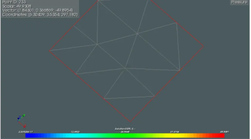
To represent a computer simulation model, it was developed a study (STUDY 5) showing a sphere of given material containing a box of different material, colliding against a rigid flat plane. Deformation, acceleration and velocity were evaluated under dynamic conditions.
Finally, the last preliminary test (STUDY 6) was equal to the previous study, but with shorter sampling time. The aim of the study was to analyse with greater detail the values of deformation and acceleration during the first impact between sphere and plane.
3.6
The experimental activity at ATB
Laboratory tests at Potsdam were aimed at measuring the impact force pro-duced by two artificial fruits when dropped on a base provided with sensors. The two artificial fruits were of spherical form and with different mass, diam-eter, density and modulus of elasticity.
The first, named “BALL 1” or BIG BALL (Figure 3.1), had diameter of 68.4 mm (average value in the three axial directions: x = 68.4 mm, y =
68.3 mm, z=68.6 mm), mass of 57 g and then density of 338 kg/m3.
The second, named “BALL 2” or SMALL BALL (Figure 3.1), had diameter of 57.4 mm (average value in the three axial directions: x = 58.2 mm, y =
57.1 mm, z=57.0 mm), mass of 134 g and then density of 1350 kg/m3. A summary of the main characteristics of the two spheres is reported in Table 3.1.
Table 3.1: Main features of the two artificial fruits. Artificial fruits Diameter, mm Mass, g Density, kg/m3
BALL 1 68.4 57 338
Figure 3.1: The two artificial fruits used for the drop tests: BALL 1 (left) and BALL 2 (right).
3.6.1
Measurement of the modulus of Young
The two spheres were preliminarily studied with a “texture analyser” (Figure 3.2), an instrument that records the curve stress-strain, from which it can be obtained the modulus of Young based on the Hertz theory.
To this end, the texture analyser was equipped with two spherical steel probes of different diameter (Figure 3.3) to press the artificial fruits. The two probe diameters were:
• probe 1: diameter = 12.7 mm; • probe 2: diameter = 6.3 mm.
Ten points, enumerated in ascending order from 1 to 10, were located at random on each artificial fruit. Then the two spheres were fixed in a sand bed (Figure 3.4) and pressed with the probes in correspondence of the points previously fixed at a rate of 10 mm/min until a maximum force of 2 N was reached. During the test, the instrument recorded the maximum force and the displacement at the maximum force. The force limit of 2 N ensured that the relation between force and displacement stayed approximately linear during the movement of the probe. The measurements were performed one by one during approximately one hour.
According to Hertz’s theory of elastic contact (Nuovo Colombo, 1985; Khodabakhshian and Emadi, 2011; Geyer et al., 2009), when two elastic
Figure 3.2: The texture analyser for calculating the modulus of Young.
spheres with diameters D1 and D2 are are brought into contact at a single
point, if collinear forces F are applied so as to press the two spheres together, deformation takes place and a small contact area will replace the contact point of the unloaded state (Figure 3.5).
Hertz starts by assuming that the contacting solids are isotropic and linearly elastic, and also that the representative dimensions of the contact area are very small compared to the various radii of curvature of the undeformed bodies, in the vicinity of the contact interface.
move-Figure 3.3: Spherical probes for measur-ing the modulus of Young.
Figure 3.4: Positioning of the sphere for measuring the modulus of Young.
Figure 3.5: Hertz contact of two spheres.
ment of approach along the line of the applied force of two points, each of which in one of the two bodies, can be evaluated as:
u=1.0403 F2C2 E CC , (3.1) being:
• F: total force which presses the bodies against one another; • CE = 1−ν12 E1 +1−ν 2 2 E2 ;
• 1 CC = 1 D1 + 1 D2
: a parameter that takes into account the curvature of the two spheres;
• ν1, ν2: moduli of Poisson of the two spheres;
• E1, E2: moduli of Young of the two spheres;
• D1, D2: diameters of the two spheres.
Equation 3.1 can be solved to obtain CE:
CE = 1−ν12 E1 +1−ν 2 2 E2 = u3C C 1.0403F2 (3.2)
Assuming the sphere 1 as the probe and the sphere 2 as the artificial fruit, E1is much higher than E2, so the term
1−ν12
E1
can be neglected and Equation 3.2 allows calculation of E2: E2 =1.061 F(1−ν22) u3/2C1/2 C , (3.3) or (ASAE Standards, 1999): E2 =1.061 (1−ν22)F u3/2 1 D1 + 1 D2 1/2 . (3.4)
The value used for ν2was 0.49.
3.6.2
Drop tests with artificial fruits
After calculation of modulus of Young, the two artificial fruits were subjected to impact tests by using a drop simulator to control the impact dynamic (Figure 3.6, Geyer et al., 2009).
It consisted of a frame with two vertical guide wires, taut clamped in parallel. A sliding carriage was free to move along the guide wires. An artificial fruit was placed on a circular hole in the middle of the carriage (thickness of 5 mm). The artificial fruits protruded slightly from the hole
Figure 3.6: Schematic view of the drop simulator (Geyeret al., 2009): a = artificial fruit, b = sliding carriage, c = guide wire, d = frame, e = steel plate, and f = force sensor.
depending on their radius of curvature. The diameter of the hole (40 mm) was wider than that of a circular plate (diameter 30 mm) that was rigidly coupled on a force sensor at the bottom of the frame.
Two impact materials were considered (Figure 3.7): • Steel plate: thickness of 5 mm;
• PVC plate: thickness of 5 mm, applied over the steel plate.
The carriage was fixed at the preselected height and was released after placing the artificial fruit. Two drop heights were considered (10 cm and 25 cm) and 20 replicates for each test condition were carried out. During the impact on the plate, the force sensor recorded and stored on a PC the maximum force. The files are in tabular format and can be easily managed with a spreadsheet.
Figure 3.7: The two impact materials: steel and PVC.
3.7
Drop test simulations
The drop tests with the artificial fruits were simulated with Salome-Meca and Code-Aster, using as moduli of Young for the artificial fruits those measured with the experimental tests. The aims of these simulations were to develop a model that, if in agreement with the experimental results, could be used for further simulations.
The impact area was modelled as a disk with diameter of 5 cm and thick-ness of 0.5 cm. When necessary, it was covered with a disk of PVC of same diameter and thickness.
As these preliminary simulations provided good agreement between measured and simulated impact force, the model was used to develop an extensive set of simulations to analyse the effects on the impact force of mate-rial properties (density and modulus of Young), pseudo-fruit size (spheres of different diameters) and drop height.
In detail, the experimental design considered:
• sphere diameter D: 50, 55, 60, 65, 70, 75 and 80 mm; • modulus of Young E: 0.5, 1.5, 2.5 and 3.5 MPa; • material density ρ: 900, 1000 and 1100 kg/m3;
• drop height h: 10, 15, 20, 25, 35 and 50 cm.
With the given values of material density and sphere diameter, the mass of the sphere ranged from 60 up to 295 g. All values were chosen to approach potato tubers properties (Geyer et al., 2009).
Only drop tests on steel were simulated, given their greater agreement with experimental results. Material behaviour was considered as elastic linear. The following quantities were extracted from each run test:
• the maximum impact force transmitted to the steel plate (to simulate the force sensor during drop tests);
• the maximum acceleration at the centre of the sphere (to simulate the AMU device, Figure 1.3);
• the maximum acceleration af a node of the sphere belonging to the contacting area with the steel plate.
Globally, 360 simulations were carried out, using always the same model. To reduce the simulation time, in the geometric model the sphere was placed at a distance∆h=3 mm above the impact plate and its initial velocity was calculated accordingly:
v0 =
2g(h−∆h), (3.5)
being g=9.81 m/s2the gravity acceleration and h the effective drop height. For each model, the tetrahedron containing the centre of the sphere was selected and its four nodes (N_1, N_2, N_3 and N_4) were localised. The acceleration of each node was recorded and the average values was con-sidered as representative of the acceleration of the centre of the sphere (the acceleration that should be measured by the AMU sensor).
Accelerations and impact forces were analysed at varying the model parameters: diameter, density, mass and modulus of Young of the sphere and drop height.
Data analyses and graphical representations were carried out by using the open source software R (R Core Team, 2013).
Results and Discussion
4.1
General aspects
Results discuss firstly the preliminary models aimed at gaining familiarity with the software, then the experimental tests carried out at Potsdam labora-tories to measure modulus of Young and impact force of two artificial fruits, and finally the extensive set of simulations aimed at evaluating the effects of size, density, modulus of Young of the sphere and drop height on the impact parameters (maximum impact force and maximum acceleration at the centre of the sphere).
Python code to build the models and Code-Aster commands to analyse them are also provided for a reproduction of the results.
4.2
Preliminary tests
4.2.1
Study 1
Theoretical aspects
With reference to a simple and homogeneous isotropic parallelepiped block (Figure 4.1), the Hooke’s law for linear-elastic materials, in the simplest form, is given by:
with:
• σ: stress;
• E: modulus of Young; • ϵ: strain.
Figure 4.1: Normal stress.
The strain ϵ is given by:
ϵ = ∆L
L , (4.2)
with:
• ∆L: deformation; • L: initial length.
The stress σ is given by:
σ = F
A, (4.3)
• F: applied force; • A: area.
From Equation (4.1) we obtain:
ϵ = σ
E. (4.4)
Equating Equations (4.2) and (4.4), we obtain:
ϵ= ∆L L = σ E (4.5) and then: ∆L = σ EL. (4.6)
Given stress, modulus of Young, and initial length, Equation (4.6) allows the calculation of the deformed shape.
Study 1 refers to an object parallelepiped-shaped with size (x, y and z values) 10 cm×10 cm×100 cm and modulus of Young E = 100 N/cm2. This object is placed on a plane that imposes the boundary conditions (no movements of the base); on the opposite face it is applied a force equal to 1000 N.
Being the area of application of the force A =100 cm2, from Equation (4.3) we obtain the theoretical value of stress:
σ = 1000 N
100 cm2 =10 N/cm
2. (4.7)
From Equation (4.6) we obtain the theoretical value of deformation:
∆L = 10 N/cm 2
100 N/cm2100 cm=10 cm. (4.8) Geometrical model building
The next step is the building in Salome-Meca of the model with the aim to verify the correctness of the solution provided by the software. To this
purpose it was verified the agreement between the theoretical values of∆L and σ and those calculated after the FEM analysis.
Primarily, by means of theGeometry module of Salome-Meca, it was built a box with size 10 cm×10 cm×100 cm. Salome-Meca provides some primitive entities to build models. A box can be defined by specifying two vertices (its opposite corners), or by specifying its dimensions along the coordinate axes and with edges parallel to them.
After, the box was “exploded” by using theExplode function: in this way the box is divided in its face components. Moreover, it is possible to detect the face, which was named Pressure, on which to apply the stress σ, and the face, which was namedBase, regarded as constrain. Single faces can be selected with the mouse pointer.
Meshing
The goal is now to divide the box volume into a mesh, a bunch of small volumes on which it will be applied the material properties and it will be calculated the stresses resulting from the load.
TheMesh module of Salome-Meca provides several algorithms in order to produce a mesh. The menu Mesh, Create Mesh, opens a dialogue box calledCreate Mesh. Selecting the Box value as geometrical object, you will be prompted to fill Hypothesis and Algorithm. Here there is a multiple selection for both fields. We used the algorithmNETGEN 3D-2D-1D (triangulation). A new element namedMesh_1 will be created.
Subsequently, it is necessary the designation of the faces on which it will be applied the loads and of the volumes on which it will be applied the material properties. When the mesh and all geometrical entities (faces and volumes) have been created, the mesh will be exported to aMED file format that can be read by Code-Aster.
Model processing via Code-Aster
Model processing is carried out by using a script, that is a Python code that can be edited according to the needs. There is a small utility, named
EFICAS, that enables to input the material properties, the loads, the boundary conditions and so on. EFICAS can be launched via the ASTK wizard, a graphical user interface for Code-Aster.
To assign material properties, we used theDEFI_MATERIAU directive. In a linear study, a material’s name and three numerical values are required: modulus of YoungE, Poisson coefficient NU and volumetric mass RHO. In this study the material’s name entered isMat1.
To assign load conditions, theAFFE_CHAR_MECA directive is used. To apply a boundary condition to the faceBase of our box, the DDL_IMPO instruction assigns at theGROUP_MA Base null displacement along all the three coordi-nates. To apply the homogeneous pressure to the facePressure of our box, thePRES_REP instruction assigns at the GROUP_MA Pressure the desired value of loads (10 N/cm2).
Finally, theMECA_STATIC instruction provides the solution and the fields for nodes and elements are saved in aMED file. Here is the command file. # Linear Statics with 3D linear solid elements
# template by J.Cugnoni, CAELinux.com, 2005
DEBUT();
# Read MED MESH File
# First command LIRE_MAILLAGE is used to read the MED mesh file # generated by Salome.
# To Do:
# Enter the name of your Salome Mesh in b_format_med->NOM_MED
MeshLin=LIRE_MAILLAGE(UNITE=20, FORMAT='MED', NOM_MED='Mesh_1', INFO_MED=1,);
# Assigns a physical model to geometric entities.
# are used for mechanical simulation (PHENOMENE=MECANIQUE) # with 3D solid elements.
# To Do (Optional):
# you can assign other physics or element types (like shells # for example) to some of the elements by replacing TOUT=OUI # in AFFE with GROUP_MA = TheElementGroupYouWantToModel
FEMLin=AFFE_MODELE(MAILLAGE=MeshLin, AFFE=_F(TOUT='OUI', PHENOMENE='MECANIQUE', MODELISATION='3D',),); # Material properties # To Do:
# Enter your material properties in this section if necessary # Copy/Paste the DEFI_MATERIAU command to add a second material
Mat1=DEFI_MATERIAU(ELAS=_F(E=10, NU=0.3,
RHO=1000,),);
# Assign Material properties to Elements # To Do:
# If you need more than one material, you need to enter pairs # of element group <-> materials by duplicating the AFFE option.
Mat=AFFE_MATERIAU(MAILLAGE=MeshLin, MODELE=FEMLin, AFFE=_F(TOUT='OUI',
MATER=Mat1,),);
# This section defines the boundary conditions of the FEA, use # DDL_IMPO on selected groups to impose displacements and
# FORCE_*/PRESSION to apply forces/pressures to selected groups
# To Do:
# for each boundary conditions, you need to choose the # appropriate option, for example DDL_IMPO for imposed
# displacements, and assign this option to a selected region of # the mesh by using the GROUP_NO option for a node group or the # GROUP_MA for face/volume groups.
BCnd=AFFE_CHAR_MECA(MODELE=FEMLin, DDL_IMPO=_F(GROUP_MA='Base', DX=0.0, DY=0.0, DZ=0.0,), PRES_REP=_F(GROUP_MA='Pressure', PRES=1,),);
# Finite Element Solution
Solution=MECA_STATIQUE(MODELE=FEMLin, CHAM_MATER=Mat,
EXCIT=_F(CHARGE=BCnd,), SOLVEUR=_F(METHODE='MUMPS',
RENUM='AUTO',),);
# Compute VonMises Stress / Strain
Solution=CALC_ELEM(reuse=Solution, RESULTAT=Solution,
OPTION=('SIEF_ELNO', 'SIEQ_ELNO', 'SIGM_ELNO',),);
Solution=CALC_NO(reuse=Solution, RESULTAT=Solution,
OPTION=('REAC_NODA', 'SIEQ_NOEU', 'SIEF_NOEU', 'SIGM_NOEU',),);
# Write Results to MED file
IMPR_RESU(MODELE=FEMLin, FORMAT='MED', UNITE=80, RESU=_F(RESULTAT=Solution, TOUT_CHAM='OUI', TOUT_CMP='OUI',),); FIN(FORMAT_HDF='OUI',);
EFICAS only works on the command file; once it has been saved, one must come back toASTK to launch the Code-Aster calculation. Code-Aster runs and displays its output in a non interactive shell window.
Post-processing module
Come back to Salome-Meca, this time using the post-processor module, where you can graphically display the results saved by Code-Aster in a.RES.MED. file. By importing this file in Salome-Meca, we can display the SolutionDEPL and Solution SIGM_ELNO fields, that are the displacements and the stresses respectively.
To visualize the displacements, we can plot theDeformed Shape (Figure 4.2). The displacement values of the nodes belonging to the facePressure are 9.94 cm, very close to the theoretical value of 10 cm (Figure 4.3). Therefore the theoretical values of deformation agree with those computed by the software.
Finally, to visualize the stress, theSIGM_ELNO field allow plotting the stress distribution along the bar. A coloured box and a graduate colour map is
Figure 4.2: Deformed shape.
Figure 4.3: Displacements of the Pressure face nodes.
displayed (Figure 4.4). The colour of the box is the same along the bar and the numerical value assigned to that colour is 10 N/cm2. This confirms that the value of stress is the same in the entire box, as it should be.
4.2.2
Study 2
The aim of the Study 2 was to analyse a simple object composed of two materials. In the same time, all the steps pertaining to te building of the geometric model and its meshing were coded in a Python script, which allows for a parametrisation of the object geometry and then for fixing new values according to the needs.
It refers to an object composed of two overlapping parallelepipeds. That on the top, called Box_1, has size 10 cm×10 cm×100 cm and modulus of Young E = 100 N/cm2, while that on the bottom, called Box_2, has size 10 cm×10 cm×200 cm and modulus of Young E = 50 N/cm2. This object is placed on a plane, which imposes the constraint conditions on the base, while on the face opposite the base it is applied a force equal to 1000 N.
For each parallelepiped it was verified the agreement between theoretical values and simulated values of displacements∆L and stress σ.
Considering only theBox_2, the theoretical value of stress σ2is equal to:
σ2 = 1000 N
100 cm2 =10 N/cm
2
. (4.9)
The corresponding value∆L2of the deformation is:
∆L2 = 10 N/cm 2
50 N/cm2 ·200 cm. (4.10)
Considering only theBox_1, the theoretical value of stress σ1is equal to:
σ1 = 1000 N
100 cm2 =10 N/cm
while the theoretical value of deformation∆L1is equal to:
∆L1 =
10 N/cm2
100 N/cm2 ·100 cm. (4.12)
Really, the face of the Box_1 on which it is applied the pressure has a theoretical value of total deformation given by the sum of∆L2and∆L1:
∆L=∆L1+∆L2 =50 cm. (4.13)
The model building of the object in Salome-Meca can be executed not only via graphical interface, but also with textual interface based on Python program language. Below the Python code of the Study 2.
### Loading libraries import sys import salome salome.salome_init() theStudy = salome.myStudy ### GEOM component import GEOM import geompy import math import SALOMEDS geompy.init_geom(theStudy) # size Box_1 DX1 = 10.0 DY1 = 10.0 DZ1 = 200.0 # size Box_2 DX2 = 10.0
DY2 = 10.0 DZ2 = 100.0
Box_1 = geompy.MakeBoxDXDYDZ(DX1, DY1, DZ1) geompy.addToStudy(Box_1, 'Box_1')
Box_2 = geompy.MakeBoxDXDYDZ(DX2, DY2, DZ2) geompy.TranslateDXDYDZ(Box_2, 0, 0, DZ1) geompy.addToStudy(Box_2, 'Box_2')
Fuse_1 = geompy.MakeFuse(Box_1, Box_2) geompy.addToStudy(Fuse_1, 'Fuse_1')
Partition_1 = geompy.MakePartition([Fuse_1], [Box_1, Box_2], [], [], geompy.ShapeType["SOLID"], 0, [], 0) [Box_1_1, Box_2_1] = geompy.ExtractShapes(Partition_1,
geompy.ShapeType["SOLID"], True) [Face_1, Face_2, Face_3, Face_4, Base, Face_6, Pressure,
Face_8, Face_9, Face_10, Face_11] = geompy.ExtractShapes(Partition_1, geompy.ShapeType["FACE"], True)
geompy.addToStudy(Partition_1, 'Partition_1')
geompy.addToStudyInFather(Partition_1, Pressure, 'Pressure') geompy.addToStudyInFather(Partition_1, Base, 'Base')
geompy.addToStudyInFather(Partition_1, Box_1_1, 'Box_1') geompy.addToStudyInFather(Partition_1, Box_2_1, 'Box_2')
### SMESH component
import smesh, SMESH, SALOMEDS import NETGENPlugin
NETGEN_2D3D = Mesh_1.Tetrahedron(algo=smesh.FULL_NETGEN) NETGEN_3D_Parameters = NETGEN_2D3D.Parameters() NETGEN_3D_Parameters.SetMaxSize(2) NETGEN_3D_Parameters.SetSecondOrder(0) NETGEN_3D_Parameters.SetOptimize(1) NETGEN_3D_Parameters.SetFineness(4) isDone = Mesh_1.Compute()
Box_1_2 = Mesh_1.GroupOnGeom(Box_1_1, 'Solid_1', SMESH.VOLUME) Box_2_2 = Mesh_1.GroupOnGeom(Box_2_1, 'Solid_2', SMESH.VOLUME) Base_1 = Mesh_1.GroupOnGeom(Base, 'Base', SMESH.FACE)
Pressure_1 = Mesh_1.GroupOnGeom(Pressure, 'Pressure', SMESH.FACE)
Box_1_2.SetName('Box_1') Box_2_2.SetName('Box_2')
[Box_1_2, Box_2_2, Base_1, Pressure_1] = Mesh_1.GetGroups()
# Set object names
smesh.SetName(Mesh_1.GetMesh(), 'Mesh_1')
smesh.SetName(NETGEN_2D3D.GetAlgorithm(), 'NETGEN_2D3D') smesh.SetName(NETGEN_3D_Parameters, 'NETGEN 3D Parameters') smesh.SetName(Box_1_2, 'Box_1')
smesh.SetName(Box_2_2, 'Box_2') smesh.SetName(Base_1, 'Base')
smesh.SetName(Pressure_1, 'Pressure')
The script is interpreted by Salome-Meca, so performing the geometrical building of the object and its meshing.
The Code-Aster command file is the following: DEBUT();
FORMAT='MED', NOM_MED='Mesh_1', INFO_MED=1,); FEMLin=AFFE_MODELE(MAILLAGE=MeshLin, AFFE=_F(TOUT='OUI', PHENOMENE='MECANIQUE', MODELISATION='3D',),); Mat1=DEFI_MATERIAU(ELAS=_F(E=100, NU=0.3, RHO=1000,),); Mat2=DEFI_MATERIAU(ELAS=_F(E=50, NU=0.3, RHO=1000,),); Mat=AFFE_MATERIAU(MAILLAGE=MeshLin, MODELE=FEMLin, AFFE=(_F(GROUP_MA='Box_1', MATER=Mat1,), _F(GROUP_MA='Box_2', MATER=Mat2,),),); BCnd=AFFE_CHAR_MECA(VERI_NORM='OUI', MODELE=FEMLin, DDL_IMPO=_F(GROUP_MA='Base', DX=0.0, DY=0.0, DZ=0.0,), PRES_REP=_F(GROUP_MA='Pressure', PRES=10,),);