QUADERNI DEL DIPARTIMENTO DI ECONOMIA POLITICA E STATISTICA
Marwil J. Dávila-Fernández Serena Sordi
Distributive cycles and endogenous technical change in a BoPC growth model
Distributive cycles and endogenous technical change in
a BoPC growth model
Marwil J. Dávila-Fernández
Serena Sordi
Department of Economics and Statistics
University of Siena
October 2017
Abstract
Our purpose in this paper is to expand Goodwin’s (1967) distributive cycle model to an open economy framework in a way that incorporates the balance-of-payments con-straint on growth. We do so by allowing technical change to be endogenous to the cyclical dynamics of the system and by adopting an independent investment function. We show that a Hopf-Bifurcation analysis establishes the possibility of persistent and bounded cyclical paths both for a 3D and a 4D extension of the model. Some numerical simula-tions are performed based on the analytical models developed. Motivational empirical evidence is also provided for Thirlwall’s law and the respective adjustment mechanism using a sample of 17 OECD countries.
Keywords: Growth cycle; Goodwin; Thirlwall’s law; Kaldor-Verdoorn; Distributive cycles; Hopf bifurcation.
JEL:E12; E32; O40
1
Introduction
Goodwin’s (1967) distributive cycle model has reached its …ftieth anniversary. In spite of its vintage, the model continues to be a fruitful and powerful “system for doing macro-dynamics”. In the last …fty years, more than one hundred contributions have tried to generalise its formu-lation in all possible directions and the mathematical structure of the model has been used as a basic framework to study di¤erent dimensions of capitalism’s structural instability. It must be noted, however, that with the exception of the high-dimensional Keynes-Metzler-Goodwin (KGM) system put forward by Asada, Chiarella, Flaschel and Franke (e.g. Asada et al, 2003), most existing e¤orts have been based on a closed economy set up. Needless to say, in the real world, economies are open to international trade and there are complications in applying analytical results based on the assumption of a closed economy.
When studying distributive dynamics in open economies, a particularly important problem arises that has not been discussed in the KGM literature and that we consider to deserve a careful analysis. The reason for this is that one of the most in‡uential empirical regularities in the Kaldorian growth literature –namely, Thirlwall’s rule (or law) –states that, in the long-run, growth is subject to the balance-of-payments constraint (BoPC). Given that countries cannot systematically …nance increasing balance-of-payments imbalances it implies that there is an adjustment in aggregate demand that constrains growth (Thirlwall, 1979, 2011).
Our purpose is to investigate such adjustment mechanism and its distributive implications over the cycle. In order to do so, we expand the original growth cycle set up to an open economy framework in a way that incorporates the external constraint. Furthermore, it is our aim to do this by allowing technical change to be endogenous to the cyclical dynamics of the system.
The importance of our contribution lies in providing a base-line model to study distribu-tive dynamics in open economies. In this sense, our exercise has some similarities with the pioneering work of Blecker (1989) and more recently Sasaki et al (2013), among others. Still, these contributions start from a Kaleckian framework which is di¤erent from the perspective adopted here. We consider our approach preferable for at least three reasons. First, cycles are rooted in the functioning of labour markets. This contrasts with traditional Kaleckian models that give marginal attention to the labour market. Second, even though the growth cycle set up does not explicitly di¤erentiate between long and short run, its dynamics recall Kalecki statement “the long run trend is but a slowly changing component of a chain of short run sit-uations; it has no independent entity” (Kalecki, 1968, p. 5) –a statement frequently ignored in latter formalizations of the Polish economist. Finally, we do not rely in the controversial Keynesian stability condition.
Introducing demand constraints means that any assumption of a constant or full rate of capacity utilisation cannot hold anymore. Hence, the basic motion of the system includes, besides the employment rate and the wage-share, also the rate of capacity utilisation. We show that without having to impose any special condition on the values of the parameters, a Hopf-Bifurcation analysis establishes the possibility of persistent and bounded cyclical paths for the resulting 3-dimensional non-linear dynamic system providing insights to enable better understanding of the nature of real-world ‡uctuations.
While the hypothesis of equilibrium in the balance-of-payments is plausible for the long-run, in the short-term growth might deviate from the external constraint. Therefore, we also allow for such deviations by developing a 4-dimensional dynamic system that is fully embedded in Goodwin’s fundamental insight that trend and cycle are indissolubly fused. In this second case,
function. Some numerical simulations are performed based on the analytical models.
The paper is organised as follows. In the next section we brie‡y review the original for-mulation of Goodwin’s distributive cycle model. Section 3 presents our …rst extension of the model in which we no longer have full capacity utilisation and the rate of growth of output always follows the BoPC. In section 4 we allow growth to deviate from the external constraint and, therefore, we are also able to introduce an independent investment function. Some …nal considerations follow.
2
The original formulation
In his growth cycle paper, Goodwin (1967) aimed at building a model capable of generating cycles in the growth rate of output rooted in the functioning of the labour market and the dynamics of distributive con‡ict. To concentrate on this point, he assumed full capacity utilisation so that the Keynesian principle of e¤ective demand plays no role. The model was originally conceived for a closed economy without government. For expositional purposes we can divide it into two blocks of equations: (i ) supply conditions, and (ii ) distributive conditions.
2.1
Supply conditions
Consider the following production function:
Y = minfKu; qNeg
where Y is output, K stands for capital, u in the absence of better nomenclature stands for e¤ective capacity utilisation, q is labour productivity, N is total labour force, and e is the employment rate. E¤ective capacity utilisation is given by (Y =Y )(Y =K) with Y as produc-tion at full capacity. That is, e¤ective capacity utilizaproduc-tion equals actual capacity utilizaproduc-tion multiplied by capital productivity when all machines and equipment are employed. This is the same as saying that u is given by actual capital productivity, Y =K; or the inverse of the actual capital-output ratio, (K=Y ) 1. Notice that in Goodwin (1967), Y =Y was supposed to be equal to one so that e¤ective and actual capacity are the same and u becomes simply the inverse of the capital-output ratio. Moreover, the employment rate is given by L=N , where L is the level of employment.
The Leontie¤ dynamic e¢ ciency condition states that:1
_ Y Y = _ K K + _u u = _q q + _ N N + _e e (1)
For a constant e¤ective capacity utilisation, such that uu_ = 0, and an exogenous labour force growth rate, equal to n, from (1) it follows that the rate of growth of output equals the rate of capital accumulation: _ Y Y = _ K K (2)
1For any variable x, _x indicates its time derivative (dx=dt), while ^x indicates its growth rate ( _x=x). Notice that the Leontie¤ production function is in a sense an accounting identity because Y = K Y
Y Y K = Y L N L N .
and _e e = _ Y Y _q q n (3)
i.e., variations in the employment rate are set by the di¤erence between the economy’s growth rate and the sum of labour productivity and labour force growth rates. This is equivalent to saying that the employment rate adjusts to the di¤erence between actual and (Harrod’s) natural rate of growth.
2.2
Distributive conditions
In an economy with two factors of production and no government, the income identity is: Y = wL + rK
where w and r are respectively real wages and the rate of return on capital.
Assuming that all savings come from pro…ts and that all pro…ts are reinvested we have that:
_ K
K = (1 $)u (4)
where $ = wL=Y = 1 rK=Y = w=q is the wage share. Given this assumption, there is no room in the model for an independent investment function.
Variations of real wages are given by a generic Phillips curve of the type: _
w
w = F (e), F
0( ) > 0, F00( ) 0 (5)
indicating that the bargaining power of workers increases at an increasing pace as employment expands.
Finally, from the de…nition of wage-share we have that: _ $ $ = _ w w _q q (6)
In other words, a constant functional income distribution is only possible if variations in real wages follow variations in labour productivity. As a result, distribution depends on the interaction between technology and distributive con‡ict.
2.3
The dynamic system
Substituting (4) into (2) and then the result into (3), we have: _e
e = (1 $)u _q
q n (7)
Then, substituting (5) into (6) we obtain: _ $
$ = F (e) _q
elements of a theory of economic ‡uctuations with the cycle emerging endogenously from the dynamic interaction of deterministic variables and not as the outcome of exogenous aleatory shocks.
The distributive cycle works as follows: an increase in the employment rate leads to an increase in the wage share, which decreases the pro…t share and thus capital accumulation. A reduction in capital accumulation decreases the rate of growth of output and consequently the rate of employment, leading to a decrease in the wage share and an increase in the pro…t share. The outcome of a higher pro…t share is faster capital accumulation because all pro…ts are reinvested, increasing the rate of growth of output and employment. At this point the cycle restarts. e " ) $ ") _ K K #) _ Y Y #) e # e # ) $ #) _ K K ") _ Y Y ") e "
3
A …rst extension of the model
The original growth cycle representation we have just described has been extended in a number of directions in the last …fty years.2 However, little attention has been given to possible
applications to the case of an open economy. Furthermore, Post Keynesian models have emphasised over the years the importance of demand constraints on growth. One of the most successful empirical regularities among them is Thirlwall’s rule. It proposes that since countries cannot systematically sustain increasing balance-of-payments imbalances, there is an adjustment in aggregate demand that constrains growth.3
The introduction of aggregate demand issues in an open-economy set up leaves at least four questions to be answered. First, it is not possible to assume full capacity utilisation. Second, it is not clear how the rate of employment and income distribution interact with the external constraint. Third, while the hypothesis of equilibrium in the balance-of-payments is plausible for the long-run, in the short-term growth might deviate from the external constraint and it is necessary to understand the mechanism behind this adjustment process. Finally, once we allow the rate of growth of output to deviate from the BoPC we can go further and explore the implications of using an independent investment function.
In the remainder of the paper we modify the original model in order to address these issues. This section deals with the …rst two problems. We allow for variations in e¤ective capacity utilisation while the rate of growth of output follows Thirlwall’s rule. However, we assume that the economy never deviates from the balance-of-payments equilibrium condition and investment is still determined by savings. These two last assumptions are to be relaxed in the next section. From now on the model can be divided into three blocks of equations. Besides the original (i ) supply conditions, and (ii ) distributive conditions, we now have (iii ) the external constraint.
2For a very recent review of the literature on some of the main theoretical and empirical contributions in this …eld, see Araújo et al (2017). In particular emphasis must be given to the importance of recent extensions of the model in explaining …nancial ‡uctuations and the great …nancial crisis based on Minsky’s …nancial instability hypothesis (Keen, 2013; Sordi and Vercelli, 2012, 2014).
3The idea that growth is BoPC has been a crucial component of much demand-led growth theory since at least Prebisch (1959). However, it is the role of demand in de…ning the nature of the constraint that distinguishes the approach from other growth models (Razmi, 2016). For a literature review on some of the main theoretical and empirical contributions, see Thirlwall (2011).
3.1
Supply conditions
Once e¤ective capacity utilisation is allowed to vary, from the Leontie¤ e¢ ciency condition (1) it follows that: _u u = _ Y Y _ K K (9)
i.e., the rate of change in capacity utilisation now depends on the di¤erence between the rate of growth of output and capital accumulation.
Following the Kaldorian literature, labour productivity gains are endogenous to the perfor-mance of the economy. Although the growth rate of labour supply is exogenous in our model, the growth rate of labour productivity is endogenously determined through a Kaldor-Verdoorn mechanism. This modi…cation is necessary in order to change the nature of the model from one that is supply-side determined to a more Keynesian demand-led model. Therefore, pro-ductivity gains are supposed to be a function of e¤ective capacity utilisation:4
_q
q = G(u), G
0( ) > 0 (10)
Kaldor in particular developed di¤erent ways to endogenise technological change (Kaldor, 1957, 1961, 1966). For instance, in his technical progress function he anticipated some of the basic insights behind Arrow’s learning-by-doing model. Traditional speci…cations assume G ( ) to be a linear function of the actual growth rate of the economy. We avoid this road for at least two reasons. First, a linear speci…cation is extremely arbitrary at this point in the analysis. Second, the traditional interpretation of the linear coe¢ cients has been convincingly questioned by McCombie and Sprea…co (2016) because it can be derived from a neoclassical production function.5
On the other hand, our speci…cation still captures the concept of a learning-by-doing process associated with the presence of economies of scale in the use of capital. The basic idea is that to a great extent technical progress is labour saving and capital embodied. Nevertheless, machines must be operating in order for productivity gains to be e¤ectively incorporated. Notice that since u = Y
Y Y
K there are two possible channels for e¤ective capacity utilisation
to in‡uence labour productivity. The …rst one is through an increase in the degree of utilisation of machines. Higher rates of idle capacity indicate that machinery has not been properly used leaving little room for learning-by-doing. The second one is through an increase in the productivity of machines. That is, the adoption of modern production techniques comes with spillover e¤ects on workers’productivity.
4In his inaugural lecture at the University of Cambridge, Kaldor (1966, p. 10) considered the relation between productivity and output to be “a dynamic rather than a static relationship – between the rates of change of productivity and of output, rather than between the level of productivity and the scale of output”. In this sense equation (10) is somehow an hybrid since we are establishing a link between the rate of change of productivity and the level of output.
5Needless to say that the problems of such production functions are well known. For a comprehensive discussion see Petri (2004) and Felipe and McCombie (2013). Moreover, it is easy to see that using G as a linear function of output’s growth rate makes the model completely supply side again. Suppose qq_ = 0+ 1
_ Y Y, where 0 and 0 < 1 < 1 are parameters that capture a combination of increasing returns to scale, induced and exogenous technical change, greater e¢ ciency in the use of resources, and the inter-sectoral reallocation of resources. From the Leontie¤ e¢ ciency condition (1) we have ee_ = (1 1)
_ Y Y 0 n: In steady-state _ e e= 0, hence, Y_ Y = 0+n
Sasaki (2013) has recently argued that making G a function of e would capture the view that technological change is driven by inter-class con‡ict. An increase in the employment rate is supposed to increase the bargaining power of workers and generate upward pressure on wages, leading capitalists to adopt labour saving technical changes. Di¤erent versions of the argument have been put forward by several authors (e.g. Naastepad, 2006; Dutt, 2006; Flaschel, 2015; for a review of endogenous technical change in alternative growth theories see Tavani and Zamparelli, 2017). Even though we do not deny the plausibility of such a mechanism, we are, in particular, more interested in incorporating endogenous technical progress as a learning process than as a result of inter-class con‡ict. Hein and Tarassow (2010) and Rezai (2012) are examples of contributions suggesting that the two formulations might not be incompatible.6
3.2
Distributive conditions
Keeping the income identity, once we allow the level of capacity utilisation to change, if all savings come from pro…ts and a constant share s of those pro…ts is reinvested we have that:
_ K
K = s(1 $)u (11)
Furthermore, we keep the same Phillips curve (5) for the real wage dynamics, and variations of the wage-share continue to be given by the di¤erence between the rate of growth of wages and the rate of growth of labour productivity (10).
3.3
The external constraint
Suppose the following traditional functions for exports and imports:
X = X (Z), X0( ) > 0 (12)
M = M (Y ), M0( ) > 0 (13)
where X are exports, M corresponds to imports, and Z is the rest of the world’s output. Since we are abstracting from any price considerations, the real exchange rate is supposed to be constant and does not in‡uence trade. For simplicity, it is also assumed that all trade consists in the exchanges of …nal goods. Equilibrium in trade, which in this framework approximates equilibrium in the balance-of-payments, implies:
X (Z) = M (Y ) Thus, we can easily show that:
_ Y Y = _ Z Z = yBP (14)
where = dXdZ XZ=dMdY MY is the ratio between foreign income elasticities of exports and imports, and yBP is the BoPC growth rate. Notice that (14) is nothing other than Thirlwall’s law.7
6One should note that Sasaki et al (2013) in an open economy Kaleckian model uses G(u) but maintains the inter-class con‡ict interpretation making reference to Okun’s law.
7From the equilibrium in trade condition we have X (Z) = M (Y ). Taking time derivatives this means dX
dZZ =_ dM
dY Y . This last expression is equivalent to_ dX dZ Z X X ZZ =_ dM dY Y M M Y Y . Rearranging we have_ dX dZ Z X _ Z ZX = dM dY Y M _ Y
YM . But if trade is in equilibrium and is di¤erent from zero it follows dX dZ Z X _ Z Z = dM dY Y M _ Y Y or _ Y Y = _ Z Z. Moreover, it is straightforward from Euler’s homogeneity theorem that if X and M are homogeneous functions, then is constant.
Foreign trade income elasticities are dependent upon the level of diversi…cation of the econ-omy’s productive structure. A low level of diversi…cation is associated with a high propensity to import which in turn implies a high income elasticity of imports. It is also associated with a low elasticity of exports because the economy will have few di¤erent types of goods to export in the face of increasing demand.
An extensive literature on complexity has stressed the positive relation between economic complexity and productive diversi…cation (Hidalgo et al, 2007; Hausmann et al, 2014). There-fore, can also be understood as a structural variable that captures the non-price competi-tiveness of an economy. Gouvea and Lima (2010, 2013), Romero and McCombie (2016) and Martins Neto and Porcile (2017) provide empirical evidence of such an interpretation.
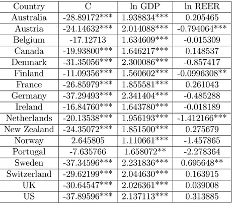
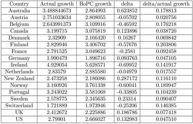
Several methodologies have been used over the years to estimate Thirlwall’s rule –which range from Ordinary Least Squares (OLS) in …rst di¤erences to Vector Error Correction (VEC) models, Fixed E¤ects (FE) models, panel Autoregressive Distributive Lag (pARDL) and Gen-eralized Method of Moments (GMM) (for a review see Romero and McCombie, 2016). Here we provide some empirical evidence of our own using the ARDL cointegration technique from a sample of 17 OECD countries between 1960 and 2016. Details of the estimation procedure and the innovative aspects of our exercise are presented in the Econometric Appendix at the end of the paper.
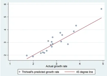
Figure 1 shows that actual and estimated growth rates are indeed very close, thus sup-porting the hypothesis that for those economies growth in the long-run follows the external constraint.
Figure 1: Actual and estimated growth rates
The Kaldorian roots of the rule derive not only from the fact that Thirlwall himself is the biographer and literary executor of the Cambridge economist but also because in his last writings Kaldor gave special attention to the role of exports in economic development. In his own words, “the rate of economic development of a region is fundamentally governed by the rate of its exports” (Kaldor, 1970, p. 342). Assuming for simplicity that X ( ) and M ( ) in (12) and (13) are homogenous functions, we have from Euler’s theorem that is constant. In the absence of the ability to attract a permanent net in‡ow of capital from abroad, the rate of growth of the economy is constrained by the requirement that it achieves current account balance.
3.4
The dynamic system
Substituting (10) and (14) into (3) we have: _e
e = yBP G(u) n or
_e = [yBP G(u) n] e = f1(e; $; u) (15)
Variations in the rate of employment are entirely determined by aggregate demand dynamics. On the one hand, the external constraint rules the rate of growth of output. Thus, a relaxation of the BoPC increases employment. On the other hand, labour productivity follows our learning-by-doing mechanism. Therefore, an increase in the rate of e¤ective capacity utilisation actually reduces employment through an increase in productivity. This of course is a partial e¤ect since u itself is an endogenous variable.
Making use of (5), (6) and (10), distributive dynamics become: _
$
$ = F (e) G(u) or
_
$ = [F (e) G(u)] $ = f2(e; $; u) (16)
Equation (16) is basically the same as (8) and states that variations in functional income distribution follow the di¤erence between the rate of growth of real wages and labour pro-ductivity. A stable wage-share can only be obtained if real wages grow at the same pace as productivity gains. Moreover, employment and e¤ective capacity utilisation have opposite e¤ects on the wage-share. An increase in the employment rate increases worker’s bargaining power allowing a rise in wages which in turn has a positive impact on the wage-share. On the other hand, an increase in the rate of capacity utilisation increases labour productivity through the Kaldor-Verdoorn mechanism reducing the share of wages in income.
Finally, substituting (11) and (14) into (9) we obtain the equation for the dynamics of capacity utilisation:
_u
u = yBP s(1 $)u or
_u = [yBP s (1 $) u] u = f3(e; $; u) (17)
The e¤ect of the rate of growth of output on e¤ective capacity utilisation is straightforward. Higher demand increases capacity utilisation. Nevertheless, an increase in capacity utilisation or a reduction in the wage-share decrease u. This is because both have a positive impact on capital accumulation through savings.
The dynamic system of the modi…ed model is formed by equations (15)-(17).
3.5
Equilibrium points, local stability analysis and Hopf bifurcation
In steady state _e=e = _$=$ = _u=u = 0. This gives us the following equilibrium conditions:
yBP = G(u) + n (18)
F (e) = G(u) (19)
Equation (18) shows that in equilibrium the sum of labour productivity and labour force growth rates must equal the BoPC growth rate. Nevertheless, the so called “natural rate of growth” is endogenous, pro-cyclical and determined by the external constraint as several empirical studies have shown to be the case ( León-Ledesma and Thirlwall, 2002; Libânio, 2009; León-Ledesma and Lanzafame, 2010; Lanzafame, 2014). The equilibrium condition (19) simply states that real wages and labour productivity must grow at the same rate in order for the wage share to be constant. Finally, condition (20) implies that the rate of growth of output must equal the rate of growth of the capital stock so as not to generate permanently increasing or decreasing idle capacity.
This last result is particularly compelling because it represents a simple and elegant for-mulation of “Say’s Law in reverse”. Still, we further improve it in the next section when an independent investment function is introduced. A broader discussion of the relation between yBP and capital accumulation as well as a solution with similar characteristics can be found
in Dávila-Fernández et al (2017).
Given the equilibrium conditions (18)-(20) we can state and prove the following Proposition regarding the existence and uniqueness of an internal equilibrium.
Proposition 1 The dynamic system (15)-(17) has a unique internal equilibrium point given by: e = F 1(yBP n) (21) $ = 1 yBP sG 1(y BP n) (22) u = G 1(yBP n) (23)
Proof. See Mathematical Appendix A.1.
Looking at equations (21) and (23) it is interesting to note that an increase in the rate of growth of output (which is determined by the external constraint) increases both the rate of employment and the rate of e¤ective utilisation. This relation resembles Okun’s rule. The result is also in line with recent developments of the so called “utilisation controversy”where Nikiforos (2013, 2016) in particular has demonstrated that …rms tend to utilise their capital more as output grows, conditional on the behaviour of increasing returns to scale. Moreover, a higher growth rate of the labour force is also associated with a lower rate of employment and e¤ective capacity.
Lastly, the relation between the BoPC growth rate and the wage-share is not univocal. Notice that (22) can be written as $ = 1 yBPsu and therefore d$
dyBP = du dyBP yBPs u u 2 . If @u @yBP yBP
u > s;an increase in yBP increases the wage share. This is because income distribution
is the adjustment variable that guarantees a constant rate of capacity utilisation. Higher growth increases u and if this e¤ect is too strong (above s) the wage share must be reduced in order to keep capital accumulation equal to the rate of growth of output. On the contrary, for @yBP@u yBPu < sa relaxation of the external constraint harms the wage share. In other words, for a propensity to save larger than the sensibility of u to the rate of growth of output, the wage share required to keep capacity utilization constant will be lower.
Next, we turn to the investigation of the local stability properties of the equilibrium points de…ned by equations (21)-(23).
Proposition 2 If the sensitivity of real wages to changes in the employment rate is su¢ ciently low and such that
F0(e ) < s(1 $ )u
e =
yBP
F 1(y
BP n)
the internal equilibrium (e ; $ ; u ) of the dynamic system (15)-(17) is locally asymptotically stable.
Proof. See Mathematical Appendix A.2.
However, for higher values of F0(e ), it may happen that F0(e ) > s(1 $ )u =e . Thus,
the dynamic behaviour of the model may drastically change, from the qualitative point of view, as the sensitivity of real wages to changes in e increases, with all the other parameters remaining constant. Using F0(e )as a bifurcation parameter, our purpose is now to apply the
Hopf Bifurcation Theorem (HBT) for 3D systems (see Gandolfo, 2009) to show that persistent cyclical behaviour of the variables can emerge as F0(e ) is increased.
Proposition 3 For values of F0(e ) in the neighbourhood of the critical value F0(e )HB = s (1 $ ) u
e (24)
the dynamic system (15)-(17) has a family of periodic solutions. Proof. See Mathematical Appendix A.3.
This result is in line with Goodwin’s (1967) aim of generating cycles rooted in the function-ing of the labour market and the dynamics of distributive con‡ict. Periodic solutions emerge as a result of an increase in the sensitivity of workers’wage demands to the employment rate.
3.6
Numerical Simulations
In this section, we present numerical simulations to show that the Hopf bifurcation occurring for values in the neighbourhood of F0(e )de…ned in (24) is supercritical so that the emerging
limit cycle is stable. The exercise also illustrates that, under plausible settings, the internal equilibrium and oscillations have economic meaning. To this end, we must …rst of all choose functional forms for the two behavioural equations of the model, namely, F ( ) and G ( ). We specify these functions as follows:
F (e) = a(e e) (25)
G (u) = bu (26)
where e is the rate of employment above which workers are able to obtain real wage increases. The functional form we have chosen in (25) captures the Marxian reserve army e¤ect and should not be confused with some sort of non accelerating in‡ation rate of unemployment (NAIRU).8 On the other hand, the parameter in equation (26) captures the presence of
increasing returns to scale for the labour productivity growth function. Finally, a and b are adjustment parameters.
8Notice that (25) can be obtained from Goodwin’s (1967) original formulation of the Phillips curve. Suppose F (e) = a1+ ae. Name a1 = ae. Therefore, F (e) = ae + ae = a(e e). We use the last expression for convenience.
Recalling the expressions given in equations (21)-(23), equilibrium values become: e = e + yBP n a (27) $ = 1 yBP s yBPb n 1= (28) u = yBP n b 1= (29) In order to choose plausible parameter values we have considered the evidence given in a number of empirical studies for the Phillips curve and the Kaldor-Verdoorn mechanism. They were also adjusted in order to provide outcomes with economic meaning:
yBP = 0:03105; n = 0:01; s = 0:3; = 1:17 (30)
a = 0:0372; e = 0:28986; b = 0:091522
Taking F0(e ) = a as the bifurcation parameter, these values imply that a
HB 0:0345:
Consequently, in our simulation, we used a value of a slightly higher than this.
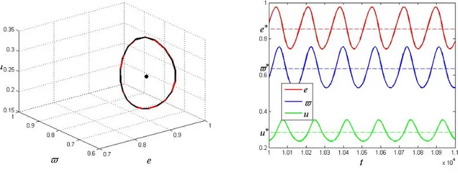
Figure 2a displays the solution path for two di¤erent initial values (e0; $0; u0) equal to
(0:92; 0:6; 0:35) and (0:77; 0:65; 0:24), both converging to the limit cycle around (e ; $ ; u ) = (0:85572; 0:63653; 0:28475). Figure 2b plots the time series of our simulations.
Figure 2a: Limit cycle 3D Figure 2b: Time series 3D
Taking a closer look at the …gures above, we can attempt to sketch a description of the dynamic interactions among the three variables along any given cycle. An increase in the employment rate leads to an increase in the wage share, which decreases the pro…t share and thus capital accumulation. A reduction in capital accumulation increases the e¤ective rate of capacity utilisation because the rate of growth of output is given and determined by Thirlwall’s rule. The increase in capacity utilisation increases the rate of growth of labour productivity through our Kaldor-Verdoorn mechanism reducing the rate of employment and the wage share, leading to an increase in the pro…t share. The outcome of a higher pro…t share is faster capital accumulation, reducing capacity utilisation and increasing the rate of
employment. At this point the cycle restarts: e " ) $ ") _ K K #) _u u ") e # e # ) $ #) _ K K ") _u u #) e "
4
A second extension of the model
As brie‡y discussed at the beginning of the previous section, while the hypothesis of equi-librium in the balance-of-payments is plausible in the long-run, for the short-run the story is di¤erent. Moreover, if we are to fully embed Goodwin’s fundamental insight that trend and cycle are indissolubly fused in our model, it is perfectly possible, as indeed is the case, that over the business cycle growth deviates from the external constraint. How actual growth adjusts to the BoPC and interacts with the rest of the dynamic system is the question we address in this section.
In an open economy without government the expenditure identity is given by: Y = C + I + X M
where C stands for consumption, I is investment, X corresponds to exports, and M stands for imports. It immediately follows that:
S I = X M (31)
with savings, S, equal to total output minus consumption.
Hence, equilibrium in the current account, X = M , implies that S = I and we have
S
K =
I
K. However, as already shown, from X = M we obtain yBP; while S
K = s(1 $)u
with $ and u determined in steady state by (22) and (23), respectively. This means that an independent investment function would actually make the model overdetermined since S and I would be equal only by chance.
Once we allow actual growth rates to deviate from the external constraint, i.e. outside equilibrium X = M does not necessarily hold, we are able to introduce an independent invest-ment function. Accordingly, the model developed must go through two important changes, one in the distributive conditions block and one in the external constraint block.
4.1
Supply conditions
There are no changes in the supply conditions of the economy. Starting from the initial Leontie¤ production function we have that variations in e¤ective capacity utilisation adjust the di¤erence between the rate of growth of output and capital accumulation. Analogously, variations in the employment rate adjust to the growth rate of the economy and variations in labour productivity. Last but not least, labour productivity continues to be modelled as a function of e¤ective capacity utilisation.
4.2
Distributive conditions
The determination of investment is central to Keynesian theories of e¤ective demand. Equa-tions (4) and (11) resulted from the assumption that all pro…ts or a share of them were
reinvested. Dropping this hypothesis opens the door to the use of an independent investment function. In this respect, the accumulation function is critical for the properties and implica-tions of the model. Unfortunately, there is considerable disagreement over the speci…cation of this function (see Skott, 2012 for a discussion of the topic).
For the purposes of this paper we adopt the following general speci…cation: I
K = H($; u), H$ < 0 and Hu > 0 (32)
The intuition of the expression above is similar to the one discussed by Bhaduri and Marglin (1990) and is recurrent in the Kaleckian literature. The basic idea is that pro…tability and capacity utilisation are used by investors as predictors of marginal pro…tability on new invest-ment and the future state of demand, respectively. According to Bhaduri and Marglin (p. 380), this investment function has the analytical advantage of separating the “demand side” impact on investment operating though the acceleration e¤ect of higher capacity utilisation from the “supply side”impact operating through the cost-reducing e¤ect of a lower real wage and higher pro…t share.
A possible alternative would be to make investment a function only of the accelerator ef-fect.9 This route is also pursued by Skott ( 1989, 2012) in a Harrodian set up. His contribution is particularly important because he presents a strong critique of the Kaleckian formulation. However, even though he makes an appealing defence of the Harrodian case, we chose to stick to equation (32). Our reasons are threefold.
First, empirical evidence does give support to the hypothesis that investment depends to some degree on the functional income distribution ( Stockhammer et al, 2009; Onaran and Galanis, 2014, 2016). Second, the model developed in this section does not rely on the extension of the standard short-run Keynesian stability condition to the long-run. That is, we do not assume that investment is less sensitive than savings to variations in the utilisation rates of capital. To the best of our knowledge, this was the main objection against the Kaleckian investment function. Finally, having H as a function of $ is required in order to generate distributive cycles in our model. A di¤erent alternative would be to assume that YY_ is a negative function of the wage-share (as does Skott). Even though we do not deny the plausibility of such a mechanism, we present an alternative one that we think better suits an open economy set up.
4.3
The external constraint
Although the BoPC growth model is addressed to the investigation of the long-run, it also has profound implications for short-run dynamics. Few studies are devoted to the analysis of how deviations from long-run paths are generated and corrected.10 What happens in an open economy if the actual growth rate causes balance-of-payments disequilibrium, which is not automatically corrected by relative prices, so that the growth of income has to adjust to bring the growth of imports and exports into line?
If the economy is growing faster than the BoPC it means imports are growing faster than exports and therefore from (31) that investment is growing faster than savings. Leaving aside any considerations about the level of international reserves of a country, if investment is
9Di¤erent speci…cations of a ‡exible accelerator can be found in the literature and of course in Goodwin himself (e.g. Goodwin, 1948, 1951; Asada et al, 2003; Chiarella et al, 2005).
growing faster than savings, then the economy is (or will be) accumulating debt. An increase in debt on the other hand is related to an increase in risk perception which indicates that at some point lenders might limit access to credit. The simple increase in risk leads to an increase in the interest rate which also contributes to a reduction of expenditure (both in terms of consumption and investment). The intensity of this adjustment depends on how creditors perceive the behaviour of the borrower. This corresponds to the traditional BoPC adjustment and in the extreme case one should expect a balance-of-payments crisis.
On the other hand, if the rate of growth of output is below what is determined by Thirlwall’s rule, exports are growing faster than imports which in turn implies that savings are growing faster than investment. In other words, the rest of the world is accumulating debt with this country. At …rst such a process could continue without limits as long as the domestic economy is willing to be a global creditor. However, two constraints might sooner or later appear. First, at some point the country might fear not being paid and force borrowers to meet their obligations. But then, imports of the debtor country will be reduced, which is equivalent to saying that exports of the surplus country will be lower, adjusting the balance of payments.
Another alternative is that the rest of the world, understanding that being in extreme debt is damaging to their interests (even politically speaking), might try to force the lender country to reduce its surplus. In this case, the economy will have to increase its expenditures increasing as a consequence its imports and restoring equilibrium in the balance of payments. This last situation resembles current negotiations led by the United States in demanding a reduction of current account surpluses by China and Germany.
A …rst approximation that represents what has been so far described is:
_y = D(yBP y); D0 > 0; and D(0) = 0 (33)
where we have set y = YY_ in order to simplify the notation.
However, from the expenditure identity it is also possible to obtain a growth rate of the economy such that (31) is always satis…ed. In reasoning with some similarities to the one presented here, Garcimartin et al (2016) called it the short-run BoPC rate of growth. Given the relations used in this paper, the rate of growth of output becomes:
y = $ 1 $ [F (e) G(u)] + h H$$+Hu_ u_ H($;u) + H($; u) i + (1 )XX_ + (1 ) (34) where = S S+M and = I I+X [0; 1].
11 Looking at the expression above, $
1 $ [F (e) G(u)]
captures the “consumption e¤ect”on growth, hH$H($;u)+Hu + H($; u)iis the “investment e¤ect”, and (1 )XX_ stands for the “foreign demand e¤ect”. Notice that exports are the only true autonomous demand component following the Kaldorian tradition.
11Equation (31) can be rewritten as S + M = I + X. Taking logarithms and time derivatives, we have a dynamic version of this macroeconomic identity given by SS_ + (1 )MM_ = II_ + (1 )XX_, where = S+MS and = I+XI [0; 1]. In our economy, savings come from pro…ts, KS = s(1 $)u. Therefore, making use of (3) and (9) we obtain that SS_ = [F (e) G(u)] 1 $$ . Moreover, from our import function, MM_ = y; where = dMdY MY is the income elasticity of imports. Finally, recall that KK_ = KI = H($; u) so that II_ =
H$$+H_ uu_
H($;u) + H($; u). Substituting those expressions in the dynamic macroeconomic condition we obtain the expression for y given in (34).
Equation (34) shows that the impact of all cyclical variables on the rate of growth of output is di¢ cult to determine. Suppose for a moment that and are constant. Then, if an increase (decrease) in the wage-share increases (decreases) consumption more than it decreases (increases) investment, the rate of growth of output will be higher (lower). In contrast, an increase in capacity utilisation only increases growth if it causes an increase in investment that overcomes the reduction in consumption. This is because an increase in u increases the rate of growth of labour productivity which in turn reduces the wage-share. Finally, variations in the rate of employment have an e¤ect similar to variations in the wage-share because they operate through the latter. Nevertheless, allowing and to vary results in signals becoming almost completely undetermined. This indeterminacy resembles the pro…t-led vs wage-led controversy in the Kaleckian literature (see Blecker, 2016 for a discussion of the topic).
It is outside the scope of this paper to take a position in the debate or propose a particular solution for that discussion. Still, it is not possible to ignore the e¤ects of cyclical variables in the adjustment process of y. Therefore we generalise (33) in order to take into account these cyclical motions and write:
_y = D(yBP y; e e ; $ $ ; u u ); with D(yBP; e ; $ ; u ) = 0
Dy < 0; De? 0; D$? 0; Du ? 0;
Deje=e = 0; D$j$=$ = 0; Duju=u = 0
where the only additional conditions we impose are that the partial derivatives of D ( ) with respect to employment, wage-share and e¤ective capacity are equal to zero at their respective equilibrium values. In other words, variations in the growth rate occur only when the system is outside equilibrium.12
4.4
The dynamic system
Substituting (10) into (3) we have: _e
e = y G(u) n
or
_e = [y G(u) n]e = g1(e; $; u; y) (35)
The interpretation of the …rst dynamic equation remains the same with the only di¤erence that now the actual growth rate of output is also an endogenous variable.
Distributive dynamics continue to be given by: _
$
$ = F (e) G(u) or
_
$ = [F (e) G(u)]$ = g2(e; $; u; y) (36)
Taking account of (9), (10) and (32), variations in e¤ective capacity utilisation are such that:
_u
u = y H($; u)
12Notice that in steady state F (e) = G(u), H$$+H_ uu_
H($;u) = 0 and H($; u) = y so that equation (34) becomes
or
_u = [y H($; u)]u = g3(e; $; u; y) (37)
An increase in demand above capital accumulation increases e¤ective capacity utilisation. The reason for this is easy to explain: production is increasing faster than the expansion of productive capacity. Notice that capital accumulation is now given by the independent investment function.
Finally, we simply restate the adjustment mechanism between the rate of growth of output and the external constraint:
_y = D(yBP y; e e ; $ $ ; u u ) = g3(e; $; u; y) (38)
Equations (35)-(38) form the dynamic system of our second modi…ed model.
4.5
Local stability analysis and Hopf bifurcation
In steady-state _e=e = _$=$ = _u=u = _y = 0. This gives us the following conditions:
y = G(u) + n (39)
F (e) = G(u) (40)
y = H($; u) (41)
0 = D(yBP y; e e ; $ $ ; u u ) (42)
The interpretation of equations (39)-(42) is very similar to the interpretation we have given for the previous model. From (40), it follows that real wages and labour productivity must grow at the same rate in order to obtain a constant wage-share. Furthermore, the rate of growth of output is such that the natural rate of growth, capital accumulation and Thirlwall’s law are equal to the former three adjusting to the last one.
In analogy with what was done with regard to the previous version of the model, we now turn to the investigation of the local stability properties of the equilibrium points. As a …rst step, we state and prove the following Proposition, regarding the conditions for a unique economically meaningful internal equilibrium.
Proposition 4 The dynamic system (35)-(38) has a unique internal equilibrium point given by:
e = F 1(yBP n) (43)
$ = H 1[yBP; G 1(yBP n)] (44)
u = G 1(yBP n) (45)
y = yBP (46)
Proof. See Mathematical Appendix A.4.
Comparing equations (43) and (45) with (21) and (23) we see that they are exactly the same. Equation (44) on the other hand comes with some novelty because of the investment function. Moreover, the net e¤ect of growth on the wage-share continues to be undetermined but now depends on the shape of the investment function. Furthermore, for a given rate of growth of output (determined by Thirlwall’s law) we obtain a rate of employment and
of capacity utilisation that depends on the bargaining power of workers and on the Kaldor-Verdoorn mechanism, respectively. After that, the income distribution will adjust in order to ensure that capital accumulation is such as to maintain the equilibrium rate of e¤ective capacity utilisation.13
Notice also that there are two ways to permanently increase the rate of employment of the economy. The …rst involves a deep transformation of the economic structure in favour of productive diversi…cation and technological complexity in order to ensure a higher yBP. The
second is related to a reduction in the bargaining power of workers. However, this second mechanism does not rely on the problematic neoclassical factor demand curves but works as follows. In order to obtain a constant wage-share, real wages and labour productivity must grow at the same rate. Highly combative workers translate small increases in employment into large increases in real wages. This means that, for a given rate of growth of labour productivity, the employment rate that ensures that real wages and productivity grow at the same rate will be lower the higher the capacity of workers to increase their wages. Therefore, a reduction in bargaining power of workers can increase equilibrium employment.
With regard to this unique internal equilibrium point, we can now state and prove the following Proposition regarding its local stability.
Proposition 5 If the sensitivity of real wages to changes in the employment rate is su¢ ciently low and such that
F0(e ) < Hu($ ; u )u
e =
Hu($ ; u )G 1(yBP n)
F 1(y
BP n)
the internal equilibrium (e ; $ ; u ; y ) of the dynamic system (35)-(38) is locally asymptoti-cally stable.
Proof. See Mathematical Appendix A.5.
Still, for higher values of F0(e ), it may happen that F0(e ) > H
u($ ; u )u =e . Thus, the
dynamic behaviour of the model may drastically change, from the qualitative point of view, as the sensitivity of real wages to changes in e increases, with all the other parameters remaining constant. We pursue a route similar to the one we have followed in the section and use F0(e )
as a bifurcation parameter in order to study the possibility of persistent cyclical behaviour. Proposition 6 For values of F0(e ) in the neighbourhood of the critical value such that
F0(e ) = Hu($ ; u )u e
the dynamic system (35)-(38) admits a family of periodic solutions. Proof. See Mathematical Appendix A.6.
Once more cyclical behavior is rooted on the labour market and distributive con‡ict.
13This last conclusion resembles Kaldor’s (1957) contribution to the “Capital Controversies”because capital accumulation was supposed to adjust to the natural growth rate through a redistribution between wages and pro…ts. At that time, however, the discussion concerned closed economies, a very di¤erent scenario from the
4.6
Numerical Simulations
We proceed by presenting a numerical simulation exercise to illustrate the existence and eco-nomic interpretation of the limit cycle whose existence was proved in the last subsection. Following what was done in section 3:6, we …rst determine functional forms for the behav-ioural equations. We maintain equations (25) and (26) for F ( ) and G ( ). Therefore, there are only two behavioural equations missing, namely, H ( ) and D ( ) for which we choose the following speci…cations:
H($; u) = c1 c2$ + c3u (47)
D (yBP y; e e ; $ $ ; u u ) = d(yBP y) + f1(e e )3 (48)
+f2($ $ )3+ f3(u u )3
where d is the adjustment parameter of the growth rate of output to the BoPC and fi with
i =f1; 2; 3g stand for the in‡uence of the other cyclical variables on growth. A cubic form for the deviations of employment, wage share and e¤ective capacity utilisation was preferred over a quadratic formulation because it allows for changes in the signal of the e¤ect if deviations occur upwards or downwards.
Recalling (43)-(46), equilibrium values become:
e = e + yBP n a (49) $ = c3 c2 yBP n b 1= +c1 yBP c2 (50) u = yBP n b 1= (51) y = yBP (52)
Parameter values were chosen in accordance with the magnitude of the ones found in several empirical studies for the Phillips curve, the Kaldor-Verdoorn mechanism, and the investment function. However, to the best of our knowledge, there are no estimates for the last equation. A careful analysis of D ( ) would have to rely on country-speci…c time series techniques because fi parameters are supposed to have a di¤erent combination of signs for di¤erent economies
(as the wage-led vs pro…t-led debate shows). Nevertheless, in order to have a preliminary approximation of these magnitudes, we estimated D ( ) using the panel built on the previous section to estimate Thirlwall’s law and assuming for a moment that fi = 0.
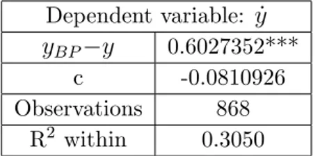
Table 1 reports the estimates of the Fixed E¤ects (FE) regression:
Dependent variable: _y yBP y 0.6027352***
c -0.0810926 Observations 868
R2 within 0.3050
Table 1: FE estimations of D( ). *,** and *** are 10%, 5% and 1% of signi…cance
A positive adjustment coe¢ cient of 0:6 is in line with the theoretical discussion presented in this section. Given that we cannot reject the null hypothesis of an intercept equal to zero even at the 10% of signi…cance, in steady state the rate of growth of output converges (or ‡uctuates) around the BoPC.
Accordingly, for the numerical simulations, we use the following parameter values, which were also adjusted in order to provide outcomes with economic meaning:
yBP = 0:03105; n = 0:01; a = 0:0422
e = 0:28986; b = 0:091522; = 1:17 c1 = 0:03061; c2 = 0:05; c3 = 0:11407
d = 0:6; f1 = 0; f2 = 0:75; f3 = 0
There are eight possible combinations of fi that can provide di¤erent cyclical dynamics.
We chose to set f1 and f3equal to zero in order to focus on income distribution. This of course
does not have necessarily to be the case. Nevertheless, it allows the model to provide some speci…c insights into the relation between the income distribution and growth. A positive f2
comes near to the so called wage-led case because over the cycle an increase in the wage share increases consumption more than it decreases investment and therefore increases the rate of growth of output. Analogously, a negative f2 approaches the pro…t-led case.
Taking F0(e ) = a as the bifurcation parameter it turns out that aHB 0:0394 and
for the simulation we used a value slightly higher than this. Figure 3a displays the so-lution path for two di¤erent initial values (e0; $0; u0; y0) equal to (0:9; 0:6; 0:4; 0:04) and
(0:77; 0:65; 0:24; 0:2) when f2 = 0:75. Both trajectories converge to the limit cycle around
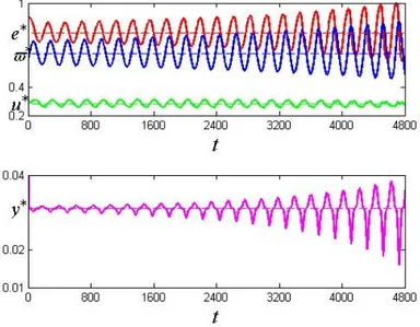
(e ; $ ; u ; y ) = (0:78868; 0:64083; 0:28475; 0:03105). Figure 3b plots the time series for the …rst trajectory. This con…rms that the Hopf bifurcation is supercritical and that, as conse-quence, the emerging persistent periodic solution is stable.
Figure 3a: Limit cycle “wage-led” economy Figure 3b: Time series “wage-led” economy
From the …gures above we can sketch a description of the dynamic interactions of the four variables over the cycle. These e¤ects can now be divided in two groups with di¤erent characteristics, which are not easy to separate. An increase in the employment rate leads to an increase in the wage share. On the one hand this reduces capital accumulation, creating pressure for an increase in capacity utilisation. On the other hand, given that an increase in the wage-share increases consumption more than it decreases investment, there is going to be an increase in the rate of growth of output which in turn creates pressure for an increase in
the narrative while the increase in utilisation brings downward pressure on employment and the wage share through the Kaldor-Verdoorn mechanism.
A reduction in the rate of employment reduces the wage share. This increases capital accumulation and ceteris paribus reduces the rate of e¤ective utilisation. Nevertheless, a reduction in the wage share reduces the rate of growth of output, bringing downward pressure on employment and capacity utilisation. The reduction in employment has the same e¤ects we have just described while a reduction in utilisation has as outcome an increase in employment and wage share because of Kaldor-Verdoorn.
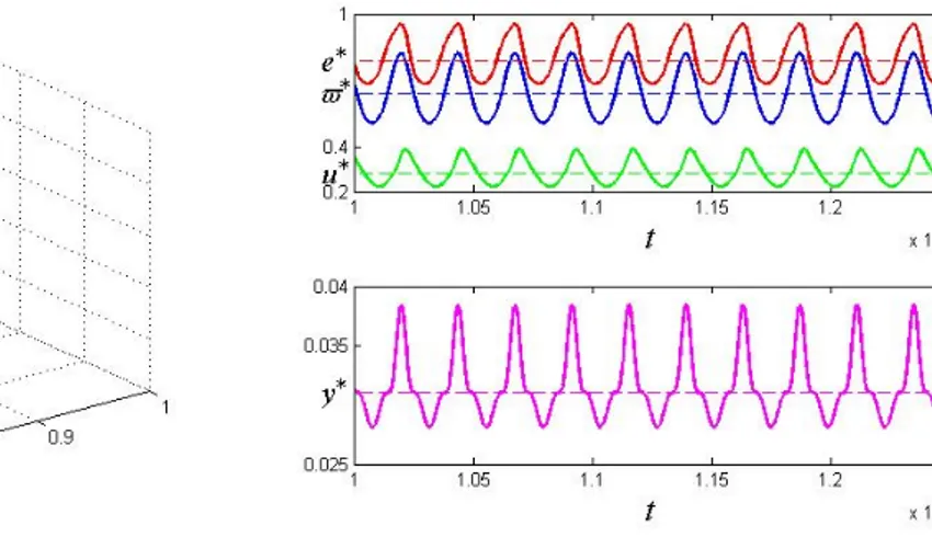
When f2 = 0:75 we were also able to …nd a supercritical Hopf bifurcation with a periodic
stable solution around the same equilibrium as before. However, the limit cycle lies outside values with an economic interpretation. Figure 4 plots the time series of our simulation for initial values (e0; $0; u0) equal to (0:9; 0:6; 0:4; 0:04).
Figure 4: Time series 4D, “pro…t-led” case
As we can see, the periodic solution increases in magnitude while slowly converging to the limit cycle outside values with economic meaning. While this result has to be taken parsimoniously, it throws a question, at least for the set of parameters and functional forms used in numerical simulations, over the sustainability of the so called pro…t-led regime that is usually claimed for open economies.
Still, two observations have to be made. First, in general pro…t-led regimes are considered to be more likely in open economies because of price-competitiveness e¤ects, while here we abstracted from any price considerations. Second, recall from the local stability analysis that for values of F0(e ) < a
HB the system actually exhibits convergence to equilibrium. Periodic
solutions emerge as a result of an increase in the sensitivity of workers’ wage demands to the employment rate. What our numerical exercise indicates is that the pro…t led regime is unsustainable only once endogenous ‡uctuations emerge, that is, for highly combative workers. A description of the dynamics follows. An increase in the employment rate increases the wage share and as consequence reduces capital accumulation and the rate of growth of output because the reduction in investment is higher than the increase in consumption. On the one hand, a reduction in capital accumulation creates upward pressure on the rate of capacity
utilisation which is expected to decrease the employment rate through Kaldor-Verdoorn. On the other hand, a reduction in the rate of growth of output creates downward pressure on capacity utilisation, which in turn is expected to increase employment. It seems that at the beginning, the …rst e¤ect prevails and we have periodic ‡uctuations within an economically meaningful range. However, the second e¤ect increases in magnitude as time goes by and the model converges to a limit cycle outside a range of values with economic meaning.
5
Conclusions
In the last …fty years Goodwin’s distributive cycle model has been and continues to be used as a fruitful “system for doing macro-dynamics”. We note, however, that most of the existing contributions have been based on a closed economy framework. In this paper we have o¤ered a modeling structure that expands the original model to an open economy framework in a way that incorporates the Balance-of-Payments constraint on growth. We have done so allowing technical change to be endogenous to the cyclical dynamics of the system.
We developed a three dimensional dynamic system that includes, besides the employment rate and the wage-share of the original model, also the rate of e¤ective capacity utilisation. We showed that without having to impose any special condition on the values of the parameters, a Hopf-Bifurcation analysis establishes the possibility of persistent and bounded cyclical paths providing insights to enable better understanding of the nature of real-world ‡uctuations.
Moreover, in order to obtain a model that is fully embedded in Goodwin’s fundamental insight that trend and cycle are indissolubly fused, we build a four dimensional dynamic system where the rate of growth of output was allowed to deviate from the external constraint. In this second case, disequilibrium in the goods market was further explored introducing an independent investment function. The importance of our contribution resides in its provision of a base-line model to study distributive dynamics in open economies.
Some numerical simulations were performed based on the analytical models. We showed that indeed under plausible conditions, a stable limit cycle emerges. Furthermore, even though our model is not Kaleckian in nature, it is possible to obtain insights that address the wage-led vs pro…t-led growth regimes. Our last growth-cycle model questions the sustainability of the so called pro…t-led regime that is usually claimed for open economy models.
A
Mathematical appendix
A.1
Proof of Proposition 1
To prove Proposition 1 we proceed in four steps. First, from equation (18) we have that G(u) = yBP n, where G : < ! < is a function monotonically increasing in u. The inverse
of G ( ) is also monotonically increasing so that u = G 1(y
BP n) is the unique equilibrium
value of e¤ective capacity utilisation.
Making use of equations (18) and (19) we obtain the rate of growth of real wages in terms of the external constrain, i.e. F (e) = yBP n, where F : < ! < is monotonically increasing
in e. Therefore, its inverse is also an increasing function and we obtain e = F 1(yBP n) as
the unique equilibrium value of the rate of employment.
The equilibrium wage-share is de…ned as the value of the wage-share that brings e¤ective capacity utilisation and the external constraint to equilibrium. Rearranging (20) it is easy to see that $ = 1 yBPsu . Substituting the equilibrium value of capacity utilisation in this last expression we arrive at $ = 1 sG 1yBP(yBP n).
Finally, in order for equilibrium values to have an economic meaning, we have to impose 0 < G 1(y
BP n) < 1, 0 < F 1(yBP n) < 1, and yBP < sG 1(yBP n).
A.2
Local stability analysis for the 3D dynamic system and proof
of Proposition 2
In this Appendix we …rst derive the characteristic equation of the dynamics system (15)-(17) and prove Proposition 2. To do this, we linearise the dynamic system around the internal equilibrium point so as to obtain:
2 4 _e _ $ _u 3 5 = 2 4 0 0 J13 J21 0 J23 0 J32 J33 3 5 | {z } J 2 4 e e $ $ u u 3 5
where the elements of the Jacobian matrix J are given by: J11 = @f1(e; $; u) @e (e ;$ ;u )= 0 J12 = @f1(e; $; u) @$ (e ;$ ;u )= 0 J13 = @f1(e; $; u) @u (e ;$ ;u )= G 0(u )e < 0 J21 = @f2(e; $; u) @e (e ;$ ;u )= F 0(e )$ > 0 J22 = @f2(e; $; u) @$ (e ;$ ;u )= 0 J23 = @f2(e; $; u) @u (e ;$ ;u )= G 0(u )$ < 0
J31 = @f3(e; $; u) @e (e ;$ ;u )= 0 J32 = @f3(e; $; u) @$ (e ;$ ;u )= su 2 > 0 J33 = @f3(e; $; u) @u (e ;$ ;u )= s(1 $ )u < 0
so that the characteristic equation can be written as
3+ b
1 2+ b2 + b3 = 0
where the coe¢ cients are given by:
b1 = tr J = J33 > 0 (53) b2 = 0 J23 J32 J33 + 0 J13 0 J33 + 0 0 J21 0 = J23J32 > 0 (54) b3 = det J = J13J21J32 > 0 (55)
The necessary and su¢ cient condition for the local stability of (e ; $ ; u ) is that all roots of the characteristic equation have negative real parts, which, from Routh–Hurwitz conditions, requires:
b1 > 0; b2 > 0; b3 > 0 and b1b2 b3 > 0:
Given (53)-(55), the crucial condition for local stability becomes the last one. Through direct computation we …nd that:
b1b2 b3 = J33J23J32+ J13J21J32 (56)
= J32(J33J23+ J13J21)
= J32[s(1 $ )u G0(u )$ G0(u )e F0(e )$ ]
= J32$ G0(u ) [s(1 $ )u e F0(e )] > 0
a condition that is satis…ed when:
F0(e ) < s(1 $ )u
e =
yBP
F 1(y
BP n)
A.3
Proof of Proposition 3
To prove Proposition 3 using the (existence part of) the Hopf Bifurcation Theorem and using F0(e ) as bifurcation parameter, we must …rst of all (HB1) show that the characteristic equa-tion possesses a pair of complex conjugate eigenvalues [F0(e )] i! [F0(e )] that become
purely imaginary at the critical value F0(e )
HB of the parameter –i.e., [F0(e )HB] = 0 –and
no other eigenvalues with zero real part exists at F0(e )HB and then (HB2) check that the derivative of the real part of the complex eigenvalues with respect to the bifurcation parameter is di¤erent from zero at the critical value.
(HB1) Given that the conditions b1 > 0, b2 > 0 and b3 are all satis…ed, in order that the
a condition which, given the expression for b1b2 b3 derived in (56), is satis…ed for
F0(e )HB = s (1 $ ) u e
(HB2) By using the so-called sensitivity analysis, it is then possible to show that the second requirement of the Hopf Bifurcation Theorem is also met. Substituting the elements of the Jacobian matrix into the respective coe¢ cients of the characteristic equation:
b1 = s(1 $ )u b2 = sG0(u )$ u 2 b3 = sG0(u )F0(e )e $ u 2 so that @b1 @F0(e ) = 0 @b2 @F0(e ) = 0 @b3 @F0(e ) = sG 0(u )e $ u 2 > 0
When F0(e )HB = s (1 $ ) u =e , apart from b1 > 0, b2 > 0 and b3 > 0 which is
always true, one also has b1b2 b3 = 0. In this case, one root of the characteristic equation
is real negative ( 1), whereas the other two are a pair of complex roots with zero real part
( 2;3 = i!, with = 0). We thus have:
b1 = ( 1+ 2+ 3) = ( 1+ 2 ) b2 = 1 2 + 1 3+ 2 3 = 2 1 + 2+ !2 b3 = 1 2 3 = 1 2+ !2 such that: @b1 @F0(e ) = @ 1 @F0(e ) 2 @ @F0(e ) = 0 @b2 @F0(e ) = 2 @ 1 @F0(e )+ 2 ( 1+ ) @ @F0(e ) + 2! @! @F0(e ) = 0 @b3 @F0(e ) = 2+ !2 @ 1 @F0(e ) 2 1 @ @F0(e ) 2 1! @! @F0(e ) = sG0(u )e $ u 2 For = 0, the system to be solved becomes:
@ 1 @F0(e ) 2 @ @F0(e ) = 0 2 1 @ @F0(e ) + 2! @! @F0(e ) = 0 !2 @ 1 @F0(e ) 2 1! @! @F0(e ) = G 0(u )e $ u 2
or 2 4 01 2 21 2!0 !2 0 2 1! 3 5 2 6 4 @ 1 @F0(e ) @ @F0(e ) @! @F0(e ) 3 7 5 = 2 4 00 sG0(u )e $ u 2 3 5 Thus: @ @F0(e ) F0(e )=F0(e ) HB = 1 0 0 0 0 2! !2 sG0(u )e $ u 2 2 1! 1 2 0 0 2 1 2! !2 0 2 1! = 2!sG 0(u )e $ u 2 4! 21+ !2 > 0
A.4
Proof of Proposition 4
The demonstration of Proposition 4 follows very closely the steps of Proposition 1. Nev-ertheless, the …rst variable to adjust is output. In equilibrium, equation (42) states that D(yBP; e ; $ ; u ) = 0; where D ( ) is monotonically decreasing in y. It follows by
construc-tion that y = yBP; e = e ; $ = $ and u = u with the employment rate, the wage share and
capacity utilization still to be determined. Once output converges to the BoPC growth rate we have from (39) that G(u) = yBP n, where G : < ! < is a function monotonically increasing
in u. The inverse of G ( ) is also monotonically increasing so that u = G 1(y
BP n) is the
unique equilibrium value of e¤ective capacity utilisation.
Making use of equations (39) and (40) we obtain the rate of growth of real wages in terms of Thirlwall’s law, i.e. F (e) = yBP n, where F : < ! < is monotonically increasing in e.
Therefore, its inverse is also an increasing function and we obtain e = F 1(y
BP n) as the
unique equilibrium value of the rate of employment.
The equilibrium wage-share is de…ned as the value of the wage-share that brings e¤ective capacity utilisation and the balance-of-payments to equilibrium. The novelty here is the independent investment function H : < ! <; monotonically increasing in u and decreasing in $. Making use of the equilibrium value of capacity utilisation and equation (42) we have that H[$; G 1(y
BP n)] = yBP. It follows that the unique equilibrium for the wage-share is
determined and de…ned by $ = H 1[yBP; $; G 1(yBP n)].
Finally, in order to obtain equilibrium values with economic meaning we have to impose 0 < G 1(y
BP n) < 1; 0 < F 1(yBP n) < 1 and 0 < H 1[yBP; $; G 1(yBP n)] < 1.
A.5
Local stability analysis for the dynamic system (35)-(38) and
proof of Proposition 5
In this Appendix we …rst derive the characteristic equation of the dynamic system (35)-(38) and prove Proposition 5. To do this, we …rst linearise the dynamic system around the internal
equilibrium point so as to obtain: 2 6 6 4 _e _ $ _u _y 3 7 7 5 = 2 6 6 4 0 0 J13 J14 J21 0 J23 0 0 J32 J33 J34 0 0 0 J44 3 7 7 5 | {z } J 2 6 6 4 e e $ $ u u y y 3 7 7 5
where the elements of the Jacobian matrix J are given by: J11 = @g1(e; $; u; y) @e (e ;$ ;u ;y ) = 0 J12 = @g1(e; $; u; y) @$ (e ;$ ;u ;y ) = 0 J13 = @g1(e; $; u; y) @u (e ;$ ;u ;y ) = G 0(u )e < 0 J14 = @g1(e; $; u; y) @y (e ;$ ;u ;y ) = e J21 = @g2(e; $; u; y) @e (e ;$ ;u ;y ) = F 0(e )$ > 0 J22 = @g2(e; $; u; y) @$ (e ;$ ;u ;y ) = 0 J23 = @g2(e; $; u; y) @u (e ;$ ;u ;y ) = G 0(u )$ < 0 J24 = @g2(e; $; u; y) @y (e ;$ ;u ;y ) = 0 J31 = @g3(e; $; u; y) @e (e ;$ ;u ;y ) = 0 J32 = @g3(e; $; u; y) @$ (e ;$ ;u ;y ) = H$($ ; u )u > 0 J33 = @g3(e; $; u; y) @u (e ;$ ;u ;y ) = Hu($ ; u )u < 0 J34 = @g3(e; $; u; y) @y (e ;$ ;u ;y ) = u > 0 J41 = @g4(e; $; u; y) @e (e ;$ ;u ;y ) = 0 J42 = @g4(e; $; u; y) @$ (e ;$ ;u ;y ) = 0 J43 = @g4(e; $; u; y) @u (e ;$ ;u ;y ) = 0 J44 = @g4(e; $; u; y) @y (e ;$ ;u ;y ) = Dy < 0
Thus, the characteristic equation for the linearised system is:
4+ b
1 3+ b2 2+ b3 + b4 = 0
where the coe¢ cients are given by:
b1 = tr J = J33 J44> 0 (57) b2 = J33 J34 0 J44 + 0 0 0 J44 + 0 J23 J32 J33 (58) + 0 J14 0 J44 + 0 J13 0 J33 + 0 0 J21 0 = J33J44 J23J32 > 0 b3 = 0 J23 0 J32 J33 J34 0 0 J44 0 J13 J14 0 J33 J34 0 0 J44 (59) 0 0 J14 J21 0 0 0 0 J44 0 0 J13 J21 0 J23 0 J32 J33 = J23J32J44 J13J21J32> 0 b4 = det J = J21J13J32J44> 0 (60)
The necessary and su¢ cient condition for the local stability of (e ; $ ; u ) is that all roots of the characteristic equation have negative real parts, which, from Routh–Hurwitz conditions, requires:
b1 > 0; b2 > 0; b3 > 0; b4 > 0 and b1b2b3 b21b4 b23 > 0:
Given (57)-(60), the crucial requirement for local stability becomes the last one. Through direct computation we …nd that:
b1b2b3 b21b4 b23 = (J33+ J44)(J33J44 J23J32)(J23J32J44 J13J21J32) (J33+ J44)2J21J13J32J44 (J23J32J44 J13J21J32)2 = | {z }J32 <0 (J13J21+ J23J33)(J33J442 + J 3 44+ J13J32J21 J23J32J44) | {z } <0
Therefore, the last Routh–Hurwitz condition is satis…ed when: J13J21+ J23J33> 0
Substituting the respective values of the Jacobian matrix:
= G0(u )e F0(e )$ + G0(u )$ Hu($ ; u )u
= G0(u )$ [e F0(e ) Hu($ ; u )u ] > 0
a condition which is satis…ed when:
F0(e ) < Hu($ ; u )u = Hu($ ; u )G
1(y
A.6
Proof of Proposition 6
To prove this proposition (see Asada and Yoshida, 2003), we must show that there exists a value
of F0(e ) = F0(e )HBsuch that we have (HB1) b1[F0(e )HB]; b2[F0(e )HB]; b3[F0(e )HB]; b4[F0(e )HB] >
0and (HB2) [F0(e ) HB] = b1[F0(e )HB]b2[F0(e )HB]b3[F0(e )HB] b1[F0(e )HB] 2b 4[F0(e )HB] b32[F0(e )HB] = 0 with d dF0(e ) F0(e )=F0(e ) HB 6= 0.
(HB1) Given the expressions for b1; b2; b3 and b4 in (57)-(60) the …rst part of the
demon-stration is immediately satis…ed.
(HB2) Through direct computation we obtain:
b1b2b3 b21b4 b23 = (J33+ J44)(J33J44 J23J32)(J23J32J44 J13J21J32) (J33+ J44)2J21J13J32J44 (J23J32J44 J13J21J32)2 = | {z }J32 <0 (J31J12+ J23J33)(J33J442 + J 3 44+ J13J32J21 J23J32J44) | {z } <0
Taking J31J12 + J23J33 and substituting the respective values of the Jacobian matrix, it is
certainly possible to …nd a F0(e ) su¢ ciently greater than Hu($ ;u )u
e such that:
J31J12+ J23J33
= G0(u )e F0(e )$ + G0(u )$ Hu($ ; u )u
= G0(u )$ [e F0(e ) Hu($ ; u )u ] < 0
and therefore b1b2b3 b21b4 b23 < 0. By continuity, this means that there exists at least one
value of the parameter F0(e ) = Hu($ ;u )u
e such that = 0 with
d dF0(e )