Modellazione numerica delle inondazioni fluviali

(1)

Università degli studi ROMA TRE

SCUOLA DOTTORALE IN INGEGNERIA

Dottorato di ricerca in Scienze dell’Ingegneria Civile

XXI Ciclo

Tesi di Dottorato

Modellazione numerica delle inondazioni fluviali

Numerical modelling of fluvial inundations

Dottorando: Ing. Pietro Prestininzi Docente guida: Prof. Guido Calenda

Coordinatore del dottorato: Prof. Leopoldo Franco Roma, Febbraio 2009

(2)

Collana delle tesi di Dottorato di Ricerca In Scienze dell’Ingegneria Civile

Università degli Studi Roma Tre Tesi n° 24

(3)

Sommario

Lo scopo di questa tesi è quello di indagare diversi possibili approcci alla modellazione numerica delle inondazioni fluviali. L’approccio modellistico matematico adottato in questo lavoro è quello maggiormente accettato per la simulazione di inondazioni su larga scala ed è basato sull’utilizzo del set di equazioni dette “delle acque basse” (SWE, Shallow Water Equations), in forma bidimensionale.

La moltitudine e la complessità dei fenomeni che intervengono nella formazione di un evento di piena impone inevitabilmente di includere nella presente indagine solo alcuni di essi. In particolare si è voluto concentrare l’attenzione sulla caratterizzazione delle modalità di propagazione di un’inondazione.

In una prima fase si sono analizzate le tipologie di eventi in cui l’onda di espansione fosse di tipo non impulsivo, mossa quindi principalmente dalla forza gravitazionale. Tale classe di fenomeni rappresenta gran parte delle inondazioni che si verificano in natura: esondazioni fluviali, inondazioni di aree costiere dovute a correnti di marea, espansioni controllate dei corsi d’acqua in bacini di laminazione, sono solo alcuni esempi. Questa restrizione operata sulla tipologia di eventi analizzati, se esclude una modesta fetta di fenomeni di interesse, consente d’altra parte di operare semplificazioni notevoli al set delle SWE. Dalla forma originaria delle SWE, rappresentata da una set di equazioni differenziali alle derivate parziali (PDE, Partial Differential Equations) di tipo iperbolico, si può dedurre un sistema semplificato di forma parabolica, (PSWE). Grazie a queste assunzioni il sistema originario, la cui soluzione numerica risulta pesante e spesso non applicabile a problemi di larga scala, diviene più facilmente gestibile e consente di allocare le risorse di calcolo resesi disponibili ad aspetti più importanti, quali ad esempio una dettagliata descrizione topografica o una più accurata modellazione delle condizioni al contorno.

La limitazione del campo di applicabilità delle PSWE, se interpretabile dal punto di vista analitico grazie ad alcune semplificazioni, non si riflette in una netta distinzione negli eventi naturali. L’eterogeneità dei fenomeni e la loro rapida evoluzione sfuma i contorni che si tenta di tracciare. E’ stato quindi necessario verificare l’accuratezza del modello non inerziale nel riprodurre un’inondazione fortemente impulsiva, simulata grazie ad un prototipo in scala. La quantificazione dell’errore derivante dal confronto con un esperimento controllato è generalizzabile a eventi su

(4)

scala reale, e consente quindi l’applicazione di tali modelli in modo più consapevole.

Una seconda parte della tesi ha riguardato lo sviluppo di un codice per la risoluzione delle SWE in forma completa adottando tecniche numeriche all’avanguardia. In particolare si è concentrata l’attenzione sulla capacità di tali modelli di simulare eventi fortemente impulsivi, nei quali si osserva la formazione e la propagazione di discontinuità nelle grandezze caratteristiche. L’approccio numerico conduce alla frontiera della ricerca in questo campo e pone problematiche stimolanti, alle cui soluzioni già proposte in letteratura si è tentato di apportare contributi innovativi. Si è indagata la capacità di mantenere un alto ordine di accuratezza anche in presenza di termini sorgente di pendenza e attrito al fondo, in concomitanza con transizioni asciutto-bagnato. L’inclusione nel modello concettuale del fenomeno del risalto idraulico, matematicamente interpretato come discontinuità e numericamente colto grazie a schemi shock-capturing, esacerba le questioni di propagazione su fondo asciutto e di gestione di topografie accidentate. La trattazione delle transizioni asciutto-bagnato è sempre risultato un aspetto critico della modellazione numerica delle SWE. Spesso le strategie adottate si sono rivelate farraginose e artificiose. Si è quindi proposto un approccio più fisicamente basato, che minimizza l’utilizzo di artifici numerici che spesso inficiano l’accuratezza propria degli complessità degli schemi numerici avanzati. Le soluzioni proposte sono quindi validate mediante il confronto con dati sperimentali e analitici.

(5)

Abstract

The scope of this thesis is to investigate different possible approaches to the numerical modelling of fluvial floods. The mathematical model adopted is most commonly used for large scale inundations, based on the bidimensional SWE (Shallow Water Equations).

The number and complexity of phenomena involved in a flood event obliges to focus only on some of them. Therefore major attention has been paid to the characterization of the modalities of propagation.

In the first part of the thesis non-impulsive inundation waves have been analyzed, where the gravitational force prevails over the inertial one. These features can be found in most of the natural flood events such as fluvial overflows, tidal inundations of coastal areas, controlled flow over flood expansion fields. Even if this restriction on the type of events excludes some of events of interest, it yields important simplifications to the SWE set. These assumptions allow to pose the original hyperbolic set of PDE (Partial Differential Equations) into a parabolic form. The complete SWE set, whose numerical solution is still computationally demanding so that its application to real cases is quite challenging, becomes more easily manageable and allows to assign the saved computational resources to the accurate modelling of some essential aspects such as the description of topography, boundary conditions and resistance forces.

The applicability restrictions of the PSWE, if theoretically deductable with some simplifications, does not provide clear criteria applicable to real world events. The extreme heterogeneity and their rapid time variability makes these criteria even more difficult to use. It then became necessary to verify the accuracy of the diffusive model when simulating a highly inertial inundation wave, reproduced with a physical experiment. The second part of the thesis deals with the development of a numerical code to solve the full dynamic form of the SWE, making use of the latest numerical techniques available. The attention has been focused on the ability of these kind of models to simulate highly impulsive floods, where the formation and the propagation of physical shocks often occur. The shock-capturing numerical approach leads to the frontier of the research in this topic and yield several issues whose solution was given some innovative contributions in this thesis. The ability of maintaining a high order of accuracy was assessed, even when source terms as bed and friction slope are to be modelled. The inclusion of the hydraulic bore modelling, mathematically interpreted as a shock, exacerbates the issues

(6)

related to the propagation over dry bed, especially when dealing with complex topography. The wet-dry transitions, always a crucial topic in the SWE numerical treatment, have been here managed in a way that minimizes the use of procedures whose lack of numerical foundation often ruins the accuracy of the overall scheme. The proposed results were then validated by means of comparisons with both experimental and analytical solutions.

(7)

List of Figures

2.1 Riemann problem and its solution in the (x, t-U) plane. Left and right wedges, red and green areas, where the initial conditions hold, star region, light blue, where the U is constant but unknown, and rarefaction

wave, in yellow, where U varies (linearly for the SWE. 16 2.2 Dependence of the applicability of simplified SWE models upon different

quantities. 22

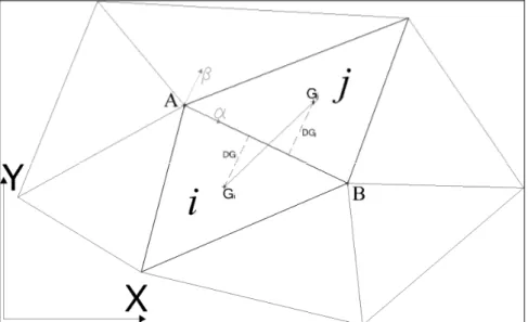
3.1 Local frame reference used to determine intercell flux: {X,Y} is the global frame reference, {a,b} is the local frame with respect to the interface (AB) between elements i and j, Gi and Gj are cells’ barycentres, DGi and

DGjtheir distance from the edge, drawn in dashed lines. 26

3.2 Stencil areas for approximation of a) longitudinal, and b) transverse water

surface slope. 28

3.3 Sketch used for friction term correction. 30 3.4 Toce river shaded view (upper panel), with location of available gauges,

mesh used for numerical simulation, approximately 16 500 elements

(lower panel). 32

3.5 Bed elevation and local slope along thalweg: average slope of the entire

valley is 1.68%. 32

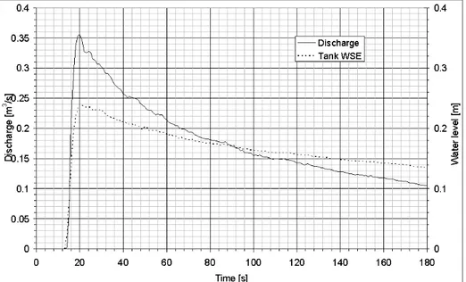
3.6 Inlet hydrographs for second scenario: the solid line is the discharge from pump record and the dashed line is the water surface elevation in the

inflow tank. 33

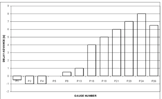
3.7 Comparison between experimental data and result of a group of numerical models: numerical data of some models are not available for all gauges. Present model results are referred to as “MOD2D”. 36 3.8 Advance or delay of front predicted by numerical model with respect to

experimental data: only thalweg gauges are considered. 37 3.9 3D view of propagation of inundation through the valley; pictures are

ordered left to right, up to bottom, and are taken at the following instants 19 – 24 – 29 – 34 – 39 – 44 – 49 – 54 – 59 – 64 s. Vertical distances are 4 times grater then horizontal ones. On very steep walls, some graphical

artefacts are visible. 38

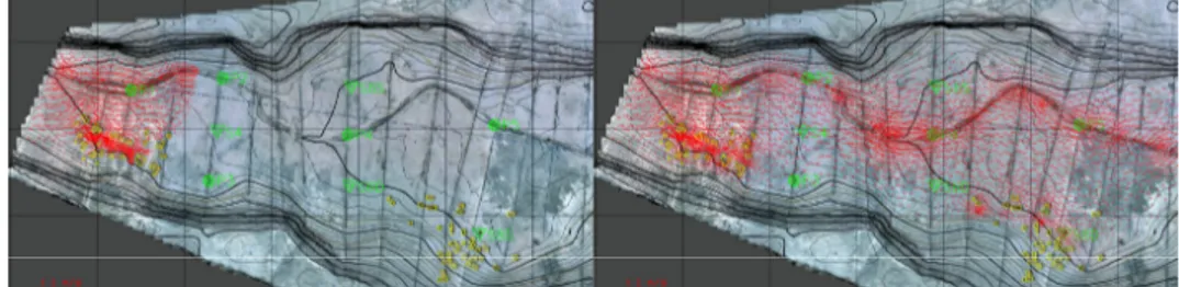
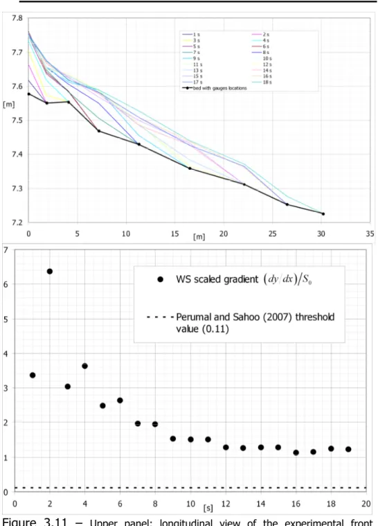
3.10 Velocity field for two frames of figure 7 (19 and 29 s): it is worth noting how the inundation does not follow the thalweg at all, and maintains a 1D dynamic with the exception of local flow between buildings. Vectors’ scale in the lower left corner. Yellow boxes are modelled buildings. 38 3.11 Upper panel: longitudinal view of the experimental front advancing over

the upstream part of the physical model; lower panel: comparison between the experimental WS scaled gradient and the threshold value

(9)

proposed by Perumal and Sahoo (2007) defining the range of applicability

of a parabolic wave model. 40

3.12 Spatial variation of maximum Froude number over the entire simulation

and its value at t=100 s. 45

4.1 Structure of the Riemann wave pattern at the interface between element i and i+1;WAF weights(in red)for application to unstructured mesh. 52 4.2 Green and blue triangles contributes to the average nodal value, used in

the non-uniform unstructured TVD gradient evaluation 57 4.3 Advancing the solution with explicit scheme, using a fractional step

method. The mechanism of formation of spurious motion starting from

still water over a sloping bed 65

4.4 Sketch of the reference used for the SWE on uneven bottom. 66 4.5 1D dam break t=1s – Case 1: wet bed; analytical solution (trace)

compared to numerical solution (circles), for depth (h), specific discharge and particle velocity (u) along x-axis (uh), Froude number 73 4.6 1D dam break t=2s – Case 1: wet bed; analytical solution (trace)

compared to numerical solution (circles), for depth (h), specific discharge and particle velocity (u) along x-axis (uh), Froude number 74 4.7 1D dam break t=1s – Case 2: dry bed; analytical solution (trace)

compared to numerical solution (circles), for depth (h), specific discharge and particle velocity (u) along x-axis (uh), Froude number 75 4.8 1D dam break t=2s – Case 2: dry bed; analytical solution (trace)

compared to numerical solution (circles), for depth (h), specific discharge and particle velocity (u) along x-axis (uh), Froude number. 76 4.9 Oblique shock test: sketch of the rectangular channel. Dark and light grey

areas are respectively lower (hu) and higher (hd) depth regions. 78

4.10 Water depth for the oblique shock test; upper panel shows a 3D view of the channel; in the middle panel 20 contours are plotted and the red line is the exact location of the shock; the lower panel shows the WSE as a

scatter field. 79

4.11 Dam break over 90° bend: schematic view of the experimental setup. 81 4.12 Dam break over 90° bend: function used to smooth the step of the bed

between the reservoir and the channel. 81 4.13 The three experimental water level series (dots), compared to numerical

results (line). 83

4.14 Water surface level for the numerical simulation at time t=14 s (colour transition from low to high levels is red Æ green Æ blue Æ purple). 84 4.15 Flow over bump - Case 1 – Water surface elevation (top) and unit

(10)

4.16 Flow over bump - Case 2 – Water surface elevation (top) and unit discharge (bottom) for the single transition case 87 4.17 Flow over bump - Case 3 – Water surface elevation (top), unit

discharge(middle)and Froude number(bottom)for the double transition

(11)

List of Tables

3.1 RMSE [m] based on depth comparison. 44

(12)

Notation

Operators: ∇⋅ →i divergence D Dti →material derivative → ∇ gradient 2 _→ ∇i laplacian k→

i partial spatial derivative along kth_direction

Symbols: ( )k _→ i kth_{element in a series} ′ → i nondimensional quantity →

i tensor (bold character for vectorial quantities)

Abbreviations:

GW → Gravity Wave

IVP → Initially Value Problem KW → Kinematic Wave

NIW → NonInertia Wave

NSE → Navier Stokes Equations ODE → Ordinary Differential Equations PDE → Partial Differential Equations

PSWE → Parabolic Shallow Water Equations SWE → Shallow Water Equations

QSW → Quasi steady Wave

Quantities:

(the ones non listed here are defined in the text) , ,

x y z → spatial coordinates

(

x y z

)

=x →

V velocity field , ,

u v w→ velocity components along spatial coordinates

(

u v w

)

=V

(13)

ρ → density p→ pressure μ → dynamic viscosity → G vector

(

0 0 g−

)

( )n

(14)

1.1 Environmental Hydraulics

Many natural systems such as sea, rivers and lakes area the places where water flows mainly in the form of free surface flows. A large amount of complex phenomena takes place in these environments and is the main topic of Environmental Hydraulics. Most of them have a close influence on humans’ everyday life, such as, water supply planning, irrigation management, pollution dispersion, erosion, biodiversity preservation, etc. Other more particular topics can be perceived as not directly influencing our lives, but are at least equally worth given close attention. Large sea currents path, flows within lakes, tsunami waves generation, inundation waves propagation, are only a few of those topics which have been considered to be essentially basic research and without a direct impact on decision planning of human activities. A change of this point of view occurred in the last decades, and is still going on, as these large scale studies have become more accessible to the average researcher. In fact when the numeric analysis, whose bases indeed date back to the 19th_{century, found its possible}

application tools in the 70’s spread of computational facilities (at least in the new continent), the research in this field was given a great acceleration. Another successive but independent occurrence that enhanced the raise of the Applied Environmental Hydraulics was the chain of hydraulic extreme events that took place in the last decade. Inundations, tsunamis, droughts, hurricanes, more and more often come to our knowledge. Is it because some sort of climate change is currently going on, is it because people are just more aware of them, is it because we are forced to interfere with them due to a lack of resources (land, water, etc.), but the world seems to be at their mercy. The reasons, though interesting and stimulating, are not the topic of this work. The duty of scientists in Environmental Hydraulics is to find mitigations to those effects, essentially predicting their occurrence, where possible, and assessing their risk. This is generally accomplished by means of a model, which is the main instrument of interpreting the reality.

(15)

1.2 Model Development and improvement

Ritengo che compito della teoria sia costruire un’immagine del mondo esterno che esiste solo in noi, che ci serva da guida in tutti i nostri pensieri ed esperimenti; cioè, per così dire, ci serva da guida nel compimento del processo di ragionamento, la cui realizzazione è, in grande, ciò che nella creazione di ogni idea in noi si compie in piccolo... La prima elaborazione e il costante perfezionamento del modello è quindi il compito principale della teoria. La fantasia è sempre la sua culla, l’intelletto vigile il suo educatore (Boltzmann, Sul significato delle teorie,

Graz 16/07/1890 ). The model is the natural way the human being perceives the reality. When the brain is stimulated by an external event, it naturally filters out all those stimulations which are thought not to be relevant for interpreting the event. This filter is mainly based on previous experiences. This unconscious process is consciously resembled every time we try to explain a natural phenomenon. The concept of model as the main tool to interpret reality can be found in Kant (1787) as the schema: it is the bridge between sensitivity and intellect which is used for processing the exterior sensible forms, by means of abstract, pure concepts of the mind. The construction of models as a basis of the comprehension is then adopted in every field of human knowledge, and has found its codification in the scientific fields. Variegated phenomena in fact require a careful and precise inspection aimed at isolating the most important features of an observable fact, and relate them to simulate it. As the understanding of the phenomenon improves, together with the methods of analysis, features are added to or taken away from the model. The power of the comprehension by means of a model is that the process is theoretically self-refining, as new information acquired improves model quality. The prediction capacities of the model are continuously compared to new events and this contrast deeply contributes to the critical appraisal of model performances and is a crucial part of the model improvement.

(16)

1.3 The role of numerical modelling in the Hydraulic Risk Assessment (HRA) field

Numerical modelling is nowadays a crucial stage in the field of Environmental Hydraulic. The developing of efficient and accurate numerical techniques, together with the large availability of computational facilities, have made numerical models accessible to designers and engineers. Numerical modelling has gained such a central role thanks to its capacity to provide the required objective characterization of many complex phenomena. Numerical models do not provide solution to problems, but can guide the designer towards optimised results, or give support to statements which, otherwise, would need to be confirmed through other much more tortuous ways (mainly physical modelling). Unfortunately, the chimera that a numerical model can be applied to complex problems in the same way a calculator is used to solve a sudoku game, is still present. The complexity of the problems for which these models are built for, forces the final users to be extremely competent in the specific field, and aware of all the assumptions which lie beneath the surface of the numerical approach.

If compared to other hydraulic fields, such as industrial processes and aerodynamics, the application of the numerical models to natural problems is relatively young. It can be dated back to the late 90s, though the mathematical characterization of the processes is much older. This delay can be due to different causes. First of all the heterogeneity of the phenomena involved force the analyst to interact with other specialists, e.g. the groundwater engineer whose research field is the contaminant diffusion must cope with the hydrogeologist and chemist. Another reason can be related to the uncertainty coming from input data, as it is generally huge for events that massively span in space and time, and these models are seldom developed to provide a stochastic characterization of results. Another factor is the deep peculiarities that distinguish every single case in environmental hydraulics: the design of an innovative foil keel shape can be carried out by means of standard, though sophisticated, numerical codes; the determination of a runoff hydrograph for a 100 km2 basin generally does not follow the same procedure employed for larger basins:

(17)

the phenomena that occur are basically the same, but scale effects are difficult to account for in a single model. Finally, as these instruments are often developed to optimize solutions in very critical fields, there is some kind of reluctance, especially on the public administration side, in adopting a tool that makes use of the latest numerical method. For the sake of truth it must be said that this unwillingness is constantly decreasing.

The HRA field is actually the composition of many other subareas, e.g. the meteorological, rainfall-runoff, underground water, fluid dynamics analysis, can all be further divided into other categories. All of these presently make large use of numerical techniques. This thesis is in the flood simulation area, whose purpose is to study the propagation of inundation waves originating from different sources: fluvial flows, rupture of retention structures, inundation of coastal areas caused by tidal oscillations. Its contents will be introduced in the next sections.

1.4 Objectives and outline of this thesis

The first attempts to apply numerical simulations to the flood propagation subject can be traced back to the 60s (Isaacson et al. 1958, Martin et al. 1969, 1971, Cunge et al. 1964, 1980, Price 1974, Katopodes and Strelkoff 1977, Abbot 1979). Notwithstanding the half century of work in the field, the topic is still “in fieri” and its evolution has undergone steep jumps in the last decade. The reasons of these sudden accelerations can be ascribed to external contributions coming from other disciplines, mainly gas dynamics. The area is still fertile to original contributions, principally oriented to analyse the applicability of the models to real scale events. A question is well likely to emerge in this context, and regards the level of complexity of the mathematical-numerical approach justifiable by the level of uncertainty of input data. Moreover this complexity needs to be even more firmly guided by the accuracy of the prediction required by the type of analysis for which the model is employed.

The almost entire research in the field of numerical simulations of flood propagation is based on the set of the SWE. This set of equations can be derived from the Navier-Stokes Equations (NSE) with some assumptions on the entity of free surface perturbations

(18)

(see section 2.1 for details). These assumptions are justified by the observation of the natural behaviour of inundation waves, where the flows involved are predominantly horizontal and the flooded areas area generally much larger than the water depth. Further observation of such phenomena reveal that a considerably large part of the flood events are characterized by spatially and temporally low variation of the velocity field. Moreover, the events where the velocity field clearly shows large gradients and fast variations, often exhibit this peculiarities only in restricted parts of their space-time domain. The SWE, indeed, account for the correct representation of this inertial behaviour, thus the aforementioned question strongly emerges: is it always necessary to include this effects in the conceptual model? Additionally, it is worth asking what payback would be gained if a model was built without including those effects. This thesis will deal with those (and more) questions in its first part: the parabolic approximation of the SWE (PSWE), which consists in neglecting the inertial contributes to the motion of a mass of fluid, is presented and discussed. A numerical model able to solve the PSWE is developed and the applicability range of the parabolic approximation is verified with the application to a controlled physical experiment.

In the second part of the thesis a further model is developed, which is able to solve the complete form of the SWE, making use of the latest numerical techniques available. The model is then validated against some analytical solutions and a laboratory experiment. The complexity of the methods required by the full dynamic version of the SWE makes the applicability of the model to large scale events more difficult, which, incidentally, justifies the use of simplified models such as the PSWE. Some new ideas to deal with the peculiar problems of the numerical methods employed to solve the SWE are presented.

(19)

2. Shallow Water Models

“Così può accadere che il matematico, continuamente occupato con le sue formule e accecato dalla loro perfezione intrinseca, prenda le correlazioni di queste fra loro per ciò che esiste veramente e distolga lo sguardo dal mondo reale (Boltzmann, Sul significato delle teorie, Graz 16/07/1890).

2.1 Deduction of the SWE set

In this chapter the SWE set will be deduced from the Navier Stokes Equations (NSE). The latter is the most general set of PDE describing the variation of the velocity field in a continuous fluid due to the action of body and surface forces. The NSE can be easily derived from the basic principles of conservation of mass and momentum. The tensorial form of the NSE for incompressible newtonian fluids is:

2 D Dt p ρ ρ ∇⋅ = μ =−∇ + + ∇ V 0 V r _G _V (2.1)

The classical way of deriving the SWE is to make some assumptions on the distribution of the velocity/pressure to simplify the integration along the vertical direction. The most straightforward is to assume a negligible vertical acceleration

0 p

w _g

t ∂z ρ

∂ = ⇒ =−_∂ _∂ (2.2)

Here a different and quite uncommon (at least in the fluvial hydraulics) approach is presented, which instead does not make any assumption on the kinematic quantities or their distribution (Mei 1999). The essence of this more elegant derivation is that it is possible to show that some peculiarities of the SWE are actually consequence of the kind of phenomena we want to model. For this purpose it is not necessary to work on the full form of the NSE: in (2.1) the viscous stress term _μ_{∇ V}2 can be dropped to obtain the

(20)

so-called Euler equations. Under the assumption of conservative mass and pressure fields acting on the fluid, the vorticity is constant in time in force of the Kelvin Theorem. If the velocity field is initially irrotational, Euler equations will keep the vorticity null through time; the scalar potential

φ

of the harmonic field

therefore satisfies Laplace equation:

V 2 ₀ φ φ =∇ ⇒∇ = V r (2.3)

as can be easily deduced using the mass continuity equation (2.1). Differentiation will be substituted by subscript notation from here on.

Aiming at solving free surface problems, eq (2.3) needs specific boundary conditions for z= ; bottom is here considered flat and η horizontal so that the corresponding boundary condition can be specified at z=−h: z t x x y y z φ η η φ η φ= + + ← = (2.4) η

(

2 2 2

)

₀ t x y z z φ φ φ φ+ + + = ← =η (2.5) 0 z z h φ = ← =− (2.6)

It is necessary to define two nondimensional parameters:

h L A h μ ε = = (2.7)

The analysis can be made clearer if the quantities are made nondimensional, so the following definitions are posed (nondimensional quantities are referred to with prime notation):

(21)

, , x y x y _L z z h A c t t_L ALc h η η φ φ ′ ′= ′= ′= = ′= (2.8)

where the velocity potential has been made nondimensional using the amplitude of potential oscillations of the linear theory (ε<<1), depending on the wave length L, the wave amplitude A, the undisturbed depth h, the linear celerity c. The derivation of nondimensional velocity components leads to the following expressions: x x y z z u u Ac Ac v _h v _h w _{L w} h h y L φ φ φ φ φ _φ ′ ′ ′ ⎡ ⎤ ⎡ ⎤ ′ ′ ⎡ ⎤ ⎡ ⎤ _⎢ _⎥ _⎢ ⎢ ⎥ ⎢ ⎥₌ ₌ _⎢ _′ _⎥₌ _⎢ _′ ⎥_⎥ ⎢ ⎥ ⎢ ⎥ _⎢ _⎥ _⎢ ⎢ ⎥ ⎢ ⎥ ⎢ ⎥ ⎢ ⎥ ⎣ ⎦ ⎣ ⎦ _′ _′⎥ ⎣ ⎦ ⎣ ⎦ (2.9)

Substituting (2.9) into (2.3), (2.4), (2.5), (2.6) , and making use of definitions (2.7) respectively results into:

(

)

(

)

2 ₀ _1, x x y y z z z μ φ′′ ′+φ′′ ′ +φ′′ ′= ← ∈ −′ εη′ (2.10)

(

)

2 z t x x y y z φ μ η εη φ εη φ′_′= ′_′+ ′ ′_{′ ′}+ ′ ′_′ _′ ← = ′ (2.11) ′ εη 2 2 2 2 0 2 z t Ag_c x y z φ φ φ φ _μ′ εη ′ ′ ′ ⎡ _⎛ ′ _⎞ ⎤ ′+ _⎢ ′ + ′ +_⎜ _⎟ _⎥= ← =′ ⎝ ⎠ ⎣ ⎦ ′ 1 (2.12) 0 z z φ′′= ← =− (2.13) ′

(22)

The essence of this approach resides in the expansion of

φ

as a power series of :

z

(

)

(

)

( )

₍

0 , , , 1n n , , n

)

x y z t z x y t φ ∞ ϕ = =

∑

+ (2.14)

the following expressions result from simple successive differentiations:

(

)

_{( )}

( )

(

)

₍

( )

₎

(

) (

)

( )

(

) (

)(

)

( ) , 0 2 , 2 2 0 1 0 2 0 1 , 1 , 1 1 1 2 1 n n x y n n n xx yy n n n z n n n zz n z x y z x y z n z n n ϕ φ ϕ φ φ ϕ φ ϕ ∞ = ∞ = ∞ + = ∞ + = ∂ = + _∂ ∂ = + ∂ = + + = + + +

∑

(2.15)

substituting (2.15) into (2.10) yields:

(2.16)

(

)

2

(

( ) ( )

)

₍

₎₍

₎

( 2) 0 1 2 1 n n n n n xx yy n z n n k μ ϕ ϕ ϕ ∞ + = ⎡ ⎤ + _⎣ + + + + _⎦

∑

144444424444443=0

As the entire sum must be null ∀ ∈ −z

(

1,εη

)

n

k

, and being independent of , it follows that each must be null, leading to a recursive definition for

n

k

z

n

ϕ

: ( ) ( )

(

)

(

)(

)

2 2 ₂ ₁ n n xx yy n _n _n n μ ϕ ϕ ϕ ₊ =− ₊ +₊ ∀ (2.17)

Using bottom boundary condition (2.13) into the third of eq (2.15) it can be shown that

ϕ

( )1

=

0

; (2.17) then allows to state that the

(23)

series has null terms for odd values of . Every term in the expansion

n

(2.14) can be thus made dependent only on

ϕ

( )0 :

( )

2

₍

₎

2 2( ) (0) 0 1 1 2 ! n n n n xy n z n μ φ ∞ ϕ = − =

∑

+ ∇ (2.18)

where the operator 2 n( )

xy

∇ means applications of Laplacian operator restricted to the

n

xy plane 2

(

)

xy xx+ yy

∇ = . It is worth noting that in the original expansion (2.14) the magnitude of each term

ϕ

_n was not a priori decreasing with (it was introduces as a Taylor expansion). This is only true in eq.

n

(2.18), provided μ< . The 1 expansion can be thus seen as a perturbation method for the potential field, with

ϕ

( )0 , the leading term, still unknown. Note

(

that

ϕ

0) is the value of

φ

at the bottom and the non dimensional

horizontal velocities are

(

)

( )0

0= u v0 0 =∇φz=−1= ∇ϕ

u r r . Substituting

derivatives of

φ

based on eq. (2.18) into surface boundary conditions (2.11) and (2.12), and writing potential spatial derivatives as function of , the expressions for the distributions of horizontal velocities and pressure along are:

0 u

z

(

)

(

)

( )

(

)

( )

(

)

(

) (

)

{

(

)

2

}

0

( )

2 2 4 0 0 2 4 0 2 2 2 2 4 0 2 1 2 1 1 1 2 z t u v z O w z O p _z _z _O c μ φ μ φ μ μ εμ 0 0 εη εη ε μ ρ =∇ = − + ∇∇⋅ + = =− + ∇⋅ + ⎡ ⎤ = − − _⎣ + − + _⎦ ∇⋅ + ∇ − ∇⋅ + u u u u r r ⎡ ⎤ ⎣ ⋅ u ⎦ u u (2.19)

It is now possible to show that the SWE are the 3D Euler equations, expanded with respect toμand truncated to the first order. This truncation obviously is allowed only if μ<< , that is the 1 perturbations can be considered “long waves”. This means that only the first terms in the right members of (2.19) are non null: the horizontal velocities are constant and equal to the velocity at

(24)

the bottom; the vertical velocity does not have any term proportional to O

( ) ( )

μ =O 1

z

−

and is therefore null; the pressure is proportional to and is null at z=

εη

, i.e. is hydrostatic. This derivation, which may, and probably is, slightly tedious, is formally more coherent to the concept of “model” explained in section 1.2 if compared to the classical ones: in fact here the purpose of the analyst, i.e. the study of long waves, is the factor that leads the search of a suitable model. Moreover it’s the observation of an evident feature (the wave length) that influences the construction of the model. The resulting model can be extended to the desired precision, just including higher order terms. The error committed neglecting each term can be evaluated as a function of wave length

μ

. The SWE are the lowest order possible.

2.2 Properties of the SWE

As seen in the previous section, the SWE are a possible solution of the NSE feasible if one is interested in studying free surface problems with depth small with respect to wave perturbations’ length. No proviso has been made on wave amplitude, so the equations derived are non linear.

In view of successive needs, it is here necessary to stress the peculiar form of the equations just derived. As stated above the NSE are derived as conservation laws of a finite mass of fluid. This means that the quantities (such as mass, momentum or energy) are balanced within a control volume. This way of deducing balance laws leads to an integral form of the equations. The equations (2.1) are indeed formulated as local or differential equations. To understand the difference between these two formulations it is possible to examine a general conservation law for a scalar in a multidimensional space: q

( )

, , ˆ q t dv ndA t_Ω _∂ ∂

_{( )}

_t Ω = ⋅

∫

x

∫

f ∂ x (2.20)

This is the natural integral form emerging from balance principles over a control volume Ω whose measure is , and is the flux

v

f

(25)

across the boundary of Ω . In general, integral forms of conservation laws are more difficult to handle, and are often recast into differential form. To obtain a differential form, eq (2.20) can be rewritten as:

( )

q ,t dv

( )

,t dv t Ω Ω ∂ _{= ∇⋅} ∂

∫

x

∫

f x (2.21)

Eq. (2.21) must be valid for any volume Ω , so the integrand of both members must be equal as well:

( )

,

(

,t

)

t

∂ q t =∇⋅

∂ x f x (2.22)

which is the differential form of the original integral law.

The crucial point is that some assumptions must be made in order to allow the derivation of (2.21) from (2.20): the functions q and must have continuous partial derivatives (i.e. must be smooth) in the volume Ω . This implies that all the functions that will develop discontinuities (such as shocks) are not solutions of

f

(2.22) while being still solutions of (2.20). This deep difference must be taken into account when such solutions are encountered.

In order to illustrate the eigenstructure of the SWE, their differential form is here recalled in terms of conserved variables

:

(

h uh vh

)

t ∂ + ∇ ⋅ = ∂ E S U = (2.23) where the vector of conserved variables is:

(2.24) 1 2 3 h u uh u vh u ⎛ ⎞ ⎛ ⎞ ⎜ ⎟ ⎜ ⎟₌ ⎜ ⎟ ⎜ ⎟ ⎜ ⎟ ⎜ ⎟ ⎝ ⎠ ⎝ ⎠ U

(26)

the matrix of fluxes is:

(

)

2 2 2 3 2 2 2 1 1 2 3 1 2 2 2 2 2 3 1 3 1 1 2 2 2 2 u u hu hv u u gu u u u hu gh huv huv hv gh u u u u u gu ⎛ ⎞ ⎛ ⎞ ⎜ ⎟ ⎜ ⎟ = = + = + ⎜ ⎟ ⎜ ₊ ⎟ _⎝ ₊ _⎠ ⎝ ⎠ E F G (2.25)

the vector of source terms is:

(

s1 s2 s3

)

=

S (2.26)

Given the SWE are spatially 2D, two different Jacobian matrices arise, namely:

( )

_{c u}20 2 ₂1 0_u ₀ uv v u ⎛ ⎞ ⎜ = − ⎜ ₋ ⎟ ⎝ ⎠ A U ⎟ (2.27)

( )

2 2 0 0 1 0 2 uv v u c v v ⎛ ⎞ ⎜ = − ⎜ ₋ ⎟ ⎝ ⎠ B U ⎟ (2.28)

where c= gh. Their eigenvalues are respectively given by:

2 1 1 2 2 1 2 3 1 x x x u u c c u u u u u u c c u λ λ λ = − = − = = = + = + 3 1 1 3 2 1 3 3 1 y y y u v c c u u v u u v c c u λ λ λ = − = − = = = + = + (2.29)

The eigenvectors _{R are the solutions to the systems:}( )i

( )i ( ) i λ = AR Ri _(2.30) ( )i ( ) i λ = BR Ri (2.31)

(27)

If a linear combination of these matrices is constructed with non-zero vectors of coefficients:

( )

=a

( )

+b

( )

C U A U B U (2.32)

the SWE system is said to be hyperbolic if the eigenvalues of C are all real, and strictly hyperbolic if, in addition, they are all distinct. These eigenvalues are easily obtainable as:

2 2 1 2 2 2 3 au bv c a b au bv au bv c a b λ λ λ = + − + = + = + + + C C C (2.33)

Thus the SWE are:

i hyperbolic if h≥ ⇒ ≥0 c 0

i.1 strictly hyperbolic for h> ⇒ ≠0 c 0 ii non-hyperbolic for 0h< ⇒ ∉ c R

From here on the x-split 2D SWE will be analysed, namely t+ x =

U F 0 (2.34)

The eigenvectors emerging from definition (2.30) and the x-eigenvalues in (2.29), are the following:

( )

₍

₎

( )

₍

₎

( )

₍

₎

1 2 3 1 1 1 2 3 2 3 1 1 1 1 1 0 0 1 1 1 u u u c v gu u u u u u c v gu u u α α β γ γ ⎛ ⎞ = − = _⎜ − _⎟ ⎝ ⎠ = ⎛ ⎞ = + = _⎜ + _⎟ ⎝ ⎠ R R R (2.35)

Not accounting for the loss of hyperbolicity due to the presence of negative non-physical depth (condition ii), condition i assures that the eigenvectors are independent so that each of them defines a

(28)

vectorial field in the phase space. For the SWE the dimension of this space is 3. Each eigenvalue defines a scalar field in the same space. In order to investigate the nature of the characteristic fields of the system of equations, it is necessary to compare the vectorial field of every eigenvector with the vectorial field defined by the gradient of the correspondent eigenvalue: if their scalar product is null, namely

( )

( )i

_{( )}

₀ i

λ

∇ U R U⋅ = ∀U (2.36)

then the characteristic field is linearly degenerate. If the two vectors are never aligned, namely:

( )

( )i

_{( )}

₀ i

λ

∇ U R U⋅ ≠ ∀U (2.37)

then the characteristic field is genuinely non-linear. Given eq. (2.29), the gradients are given by:

2 1 2 1 1 1 2 2 2 1 1 2 3 2 1 1 1 1 1 0 2 1 0 1 1 0 2 x x x u g u u u u u u u g u u u λ λ λ ⎛ ⎞ ∇ = −⎜_⎜ − ⎟_⎟ ⎝ ⎠ ⎛ ⎞ ∇ = −_⎜ _⎟ ⎝ ⎠ ⎛ ⎞ ∇ = −_⎜_⎜ + _⎟_⎟ ⎝ ⎠ (2.38)

Given the definitions (2.36) and (2.37), the SWE have a characteristic field linearly degenerate for λ₂ while eigenvalues λ₁ and λ₃ are associated with genuinely non-linear fields. The first type of fields comprises perturbations that travel with a non-linear speed s_{x y}_, =u v c, ± . The speed of the waves of the second type is instead equal to the advection velocity s_{x y}_, =u,v.

(29)

2.2.1 The Riemann problem and its solution

The wave patterns described in the previous section appear in the solution of the so-called Riemann problem.

The Riemann problem is the initial value problem defined by the augmentation of eq (2.34) and the following initial conditions:

( )

,0 0 0 L R x x x ← < ⎧ = ⎨ _{← >} ⎩ U U U (2.39)

As the above eigenstructure analysis states, three characteristic families can arise in the solution of the problem, each one associated with an eigenvalue. It is useful to illustrate the wave structure in the time-space plane as in Figure 2.1:

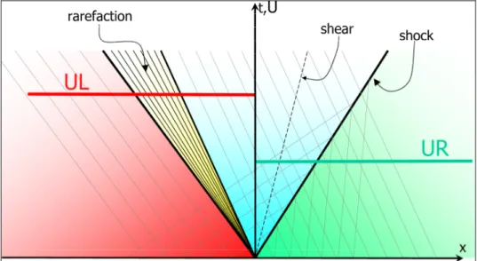
Figure 2.1 – Riemann problem and its solution in the (x, t-U) plane. Left and

right wedges, red and green areas, where the initial conditions hold; star region, light blue, where the U is constant but unknown; rarefaction wave, in yellow, where U varies (linearly for the SWE).

The lines in the space-time plot refer to discontinuities of some of the variables. The left and right states define a family of characteristic lines (light gray traces in Figure 2.1) whose slope

(30)

depends on the initial values (2.39). Obviously the left slope is generally different from right slope, thus a separation between the zones of influence of the two different conditions (2.39) must exist. This boundary is a wave in the x-t plane. The two external waves separate the x-t plane into 3 wedges: the left (right) one is the area where the initial left (right) condition still holds, thus

( ) (i.e. no information on the perturbation that took place at x=0 and t=0 has yet arrived); the solution in the middle region (called star region) is actually unknown and depends on the values of and . The two external wave can have two natures: a shock wave or a rarefaction wave (respectively a bore and a depression in the case of SWE). The respective compressive (bore) or expansive (depression) nature of the wave depends on the speeds of the characteristic fields it separates, namely the value of the two eigenvalues:

L = U U R = U U L U U_R

( ) ( )

( )

i i i Si i λ λ λ λ − + + − < ⇒ < < ⇒ U U U U rarefaction shock (2.40) where the + or – apices respectively indicate the region to the right and to the left of the wave and denotes the speed of the shock. When the characteristic lines converge, they run into the shock path, when they diverge they bound the so-called rarefaction fan. These boundaries are called head and tail of the rarefaction. In eq.

i

S

(2.40) one of the + or – regions is generally the star region so nature of the wave depends on the solution in this region. Note that the origin of this nomenclature can be traced back to the compressible gas dynamic field, so a depression, i.e. a decrease of depth, in the SWE corresponds to a decrease

of density in the gas. Across a shock wave, which is a line in the x-y

space, a jump of and occurs; no abrupt variation of occurs. The rarefaction wave is instead a wide region where a gradual variation of the and takes place, being only their x-derivatives discontinuous at the boundary of the rarefaction fan. The variable again varies continuously across this wave. The presence of the y momentum in

1 u u₂ u₃ 1 u u₂ 3 u

(2.23) allows for the presence of a third wave, which is associated with the linearly degenerate

(31)

eigenvalue λ₂ and is a shear or contact wave. It is located in the star region and all the quantities continuously vary across it, except for . Being concentrated only on the x-split of eq. u₃ (2.23), the variable here behaves like a non reactive scalar contaminant.

3

u

It is worth stressing that, being the wave patterns straight lines, the solution at each point of the x-t plane can be found as a similarity solution, that is, depends only on the ratio x/t : in other words every wedge separated by two waves indentifies a region with constant solution U.

As will be exhaustively explained in chapter 4, the Riemann problem is a building block for most numerical shock capturing numerical models.

2.3 Simplified SWE models

Although the SWE is one of the simplest mathematical model that can be derived from the NSE set, it still carries a large amount of complexity that reflects heavily on the numerical methods used to solve it. These difficulties are mainly connected to the shock development and propagation, transition between wet and dry regions, and the treatment of source terms. These topics will be covered in detail in the chapter 4.

Here a group of simplifications of the SWE will be introduced with particular attention paid to the so-called diffusive (or parabolic or noninertia) assumption. This approximation will be shown effective for the simulation of some real events in the next chapter.

For the sake of clarity the following analysis will be restricted to the 1D SWE, without loss of generality. These equations can be expressed in the form of the De-Saint Venant Equations,

( )

hu ₀ h t x ∂ ∂ ₊ ₌ ∂ ∂ (2.41)

{ { { bed slope{0 friction slope{ local convective pressure

l c p s f u u h I I u I g I g S S t x x ⎛ ⎞ ∂ ₊ ∂ ₊ ∂ ₌ _⎜ ₋ _⎟ ⎜ ⎟ ∂ ∂ ∂ ⎝ ⎠ (2.42)

(32)

The various acceleration terms in the momentum equation are weighted by different indices I, used to define the different level of approximations:

0. dynamic wave: I_l =I_c =I_p =I_s = 1

1. quasi-steady dynamic wave (QSW)

{

l 0 ₁ c p s I I ==I =I = 2. gravity wave (GW)

{

l ₀c p 1 s I I I I = = = =

3. non-inertia wave (NIW)

{

l c 0₁ p s I I I ==I == 4. kinematic wave (KW)

{

l ₁c p 0 s I I I I = = = =

All of these approximations make use of the same continuity equation (2.41).

In the following the non-inertia model will be also referred to as diffusive, dispersive or parabolic model. The nomenclature diffusive is commonly used in the hydrologic field to refer to the noninertia SWE. This can be easily explained (see section 3.1 for details) as its governing equation is similar to the diffusion of some quantity e.g. temperature diffusion (Fourier law), particles diffusion (Fick law). In general, a diffusion process is the time variation of a quantity due to the curvature of its spatial distribution.

Each of these models (1 Æ 4) applies a progressively higher level of simplification to the original equation set, and requires different boundary conditions, due to the fact that the corresponding mathematical model has a different eigenstructure.

The use of the NIW for unsteady flow routing has been increasing in recent years because it is the simplest among the approximations that can account for the downstream backwater effect and yields reasonably good results. Moreover, as demonstrated by Tsai (2003), the NIW model performs much better than the QSW, which is mathematically more adherent to the complete system: this is due to the fact that the local and convective acceleration balance each other in most of the real

(33)

world flows: neglecting only one of the two inertial terms leads to a less accurate model. In addition, the level of complexity of the solution strategies required by the quasi steady dynamic model is much higher than the diffusive model.

The theoretical assessment of the applicability of simplified versions of the SWE has been a central topic for decades, and the first attempts can be traced back to the seventies. One of the widely recognized inequality criteria was proposed by Ponce et al. (1978). The authors used a linear stability method to investigate the response of the diffusion and kinematic wave models to a periodic perturbation of a steady uniform state. They analytically compared the celerity and the attenuation characteristics (one possible formulation of the attenuation factor is δ =ln a a

(

₁ ₀

)

where and are the wave amplitudes at the beginning and at the end of a wave period) of each model with the corresponding quantities of the full dynamic model: they postulated a criterion of the NIW model to approximate the dynamic wave model within a 95% accuracy for celerity as

1

a a₀

(

)

1 2

0 0 30

TS g y ≥ (2.43)

where T is the wave period of the sinusoidal perturbation to the steady uniform flow (usually twice the time of rise of the flood wave); is the channel bed slope; S0 y the uniform flow depth. The 0

assumptions of that work were the prismatic channel and the absence of backwater effects. The latter was relaxed by Tsai (2003) who investigated the dependence of the threshold value in (2.43) on the downstream condition. Other criteria have been proposed, based on different approaches. Fread (1985) proposed his criterion based on comparisons of integrated results such as a hydrograph at the outlet of a channel:

(

)

1.6 0.2 1.2

0 51

r p

(34)

where for is the peak of the inflow hydrograph (unit discharge), the time to peak in inflow discharge, n Manning coefficient.

p

q

r

T

Ponce criterion has found its place in standard textbooks (French, 1986; Ponce, 1989; Chaudhry, 1993; Viessman and Lewis, 1996; Singh, 1996), and its effectiveness was recently assessed by Perumal and Sahoo (2007). The authors found that (2.43) consistently predicted narrower ranges of applicability of the NIW, thus its application is questionable, as other studies had previously stated (Zoppou and O’Neill, 1982; Ferrick and Goodman, 1998; Crago and Richards, 2000). The inaccuracies of the criteria are mainly connected to the linear stability analysis used to obtain them, as well as the various simplifications adopted (mainly the broad channel assumption). Perumal and Sahoo (2007), investigated the influence of the scaled water profile gradient, namely

(

dy dx S

)

₀, where y is the WSE and x is the station. This quantity was originally proposed by Henderson (1966), and used for the classification of flood waves as kinematic or diffusive. Price (1985) used it as a criterion for these approximations to be correctly applied, but gave a far too restrictive threshold of 0.05. Perumal and Sahoo (2007) stated that the upper limit of the scaled gradient should be around 0.11 for the Muskingum-Cunge method to be consistently applied.

All these criteria are summarised in Figure 2.2, where the applicability of the different wave approximations is shown dependent on the four quantities appearing in the criteria proposed above. It is clear that the condition at which no approximation of the dynamic wave should be applied is represented by a supercritical propagation of an impulsive wave over a flat, rough bed.

(35)

Figure 2.2 – Dependence of the applicability of simplified SWE models upon different quantities.

Given the numerous exceptions to the criteria developed, together with the major assumptions in their derivations, a more rigorous verification is needed. The next chapter will deal with the comparison of a highly inertial experimental flood with numerical results from a NI model.

(36)

3. Verification of applicability of

the diffusive model

In this chapter a numerical model based on the parabolic approximation of the 2D Shallow Water Equations (SWE) is presented.

It is then tested against data from a physical model of a dam break event. The choice of a real dambreak event as a comparison term for a parabolic model is due to the assumption that, given its strong inertial characterization, it would be able to highlight the limits of the diffusive approximation. The main aim is to point out at which extent this approximation is suitable for simulating such an extreme events.

3.1 Conceptual model

Diffusive approximation of (2.23) consists of neglecting local and convective accelerations in (2.24) and (2.25) leading to:

2 2 2 0 0 0 2 diff diff hu hv h gh gh ⎛ ⎞ 0 ⎛ ⎞ ⎜ ⎟ ⎜ ⎟ =⎜ ⎟ =⎜ ⎟ ⎜ ⎟ ⎜ ⎟ ⎝ ⎠ ⎝ ⎠ E U (3.1)

which can be further expanded as follows:

( ) ( ) h uh vh q t x y ∂ ∂₊ ₊∂ ₌ ∂ ∂ ∂ (3.2) 2 2 2 0 H u u v x χ h ∂ ₊ + ₌ ∂ (3.3) 2 2 2 0 H v u v y χ h ∂ + + = ∂ (3.4) whereH ≡ +h z.

The main benefit of the diffusive approximation is that, as previously stated by Hromadka and Lai (1985), the original system

(37)

of equations (2.23), in the unknown h, u, v, can be now simplified to obtain two explicit formulations u u h= ( ) v v h= ( ) coupling (3.3) and (3.4): 1 2 1 2 ˆ ( ) _x ws h u h H e S χ⋅ = ∇ (3.5) 1 2 1 2 ˆ ( ) _y ws h v h H e S χ⋅ = ∇ (3.6)

where

_{

e eˆ ˆ_x, _y

_}

is the frame reference measuring the horizontal 2D space and the quantity SWS describes the local slope of water

surface: 1 2 2 2 H H Sws H x y ⎡_⎛_∂ _⎞ _⎛_∂ _⎞ ⎤ ≡ ∇ ≡⎢_⎜ _⎟ +_⎜ _⎟ ⎥ ∂ ∂ ⎝ ⎠ ⎢ ⎝ _{⎠ ⎦}⎥ (3.7) ⎣ and results: 2 − V 2 ws S h χ = (3.8) where: V = (u,v).

(3.5) and (3.6) can be then directly substituted into (3.2) leading to:

[

k H eˆ_x

]

k H eˆ_y q t+ x ∇ + y⎡⎣ ∇ ⎤⎦= ∂ ∂ ∂ h ∂ ∂ ∂ _(3.9)

which is a single parabolic PDE in the only unknown h(x,y,t), where k is the isotropic but variable in both time and space because solution-dependent, diffusion coefficient:

(38)

2 _h2 3 χ ⋅ 1 2 ws k S = (3.10)

It is worth noting the analogy between equation (3.9) and Richards equation for flow in porous medium with trasmissivity k. Equation (3.8) implies that the model, given any topography, finds the distribution of velocities and depth that minimizes the difference between surface and friction slope.

The parabolic approximation, neglecting inertial terms, leads to a shock-free evolution, allowing the use of much simpler numerical treatments. Moreover, boundary conditions can be thus assigned in form of an imposed arbitrary depth (Dirichlet type), an imposed arbitrary source of mass (Neumann type), or a solution-dependent condition of the type q=q(h) or equivalently h=h(q) without a-priori awareness of super or sub-critical flow state needed.

As stated in many previous works (Akanbi and Katopodes,, 1988; Brufau et al. 2002; Liao et al. 2007), the critical aspect of the SWE resides in the analytical representation and numerical discretization of the friction term connected with the simulation of the advancing and receding fronts of the flood: the main problem arising when using a Chezy-type friction term is that it would grow significantly when very small depth are encountered (Horritt, 2002) as in drying and wetting areas, thus requiring the presence of a high surface slope. This fact can have a major impact on the drying phase as the depth gradient is usually opposite to bed slope so that not always negligible volumes of water remain entrapped in the thin film of water typical of SWE simulations. This is the main issue of the full dynamic model that remains qualitatively unchanged in the diffusive model.

3.2 Numerical model

The numerical scheme used here is developed from the storage cell method originally proposed by Zanobetti et al. (1970), Cunge et al. (1976) and successively used in Estrela (1994) and Romanowicz et al. (1996), Bates and De Roo (2000): in these works cells are constructed onto an equally spaced grid derived from DEM topography. Intercell fluxes are determined by means of

(39)

uniform flow formulae such as Manning and weir-type equations. Successive applications, while still dealing with rectangular grids, applied a finite difference technique to determine the fluxes based on the diffusive bidimensional scheme (Prestininzi and Fiori, 2006; Horritt and Bates, 2001). This approach has been analysed by Bates and De Roo (2000), who found that in real case applications the diffusion wave treatment employed with the storage cell method out-performed two-dimensional full dynamic finite element schemes because the simplified treatment of flow routing on the floodplain allowed a much higher density representation of floodplain topography. The simplified process representation also offers the possibility of model upscaling to much larger spatial scales, as computational limitations are reduced (Horritt and Bates, 2001).

The storage cell scheme based on structured grid, is here applied to a non-structured mesh. The method utilizes cell-centred depth values to determine fluxes at interfaces. Depth field is piecewise constant over the domain; linear variation of surface height is used in discretization of diffusive terms.

Figure 3.1 – Local frame reference used to determine intercell flux: {X,Y} is the global frame reference, {a,b} is the local frame with respect to the interface (AB) between elements i and j, Gi and Gj are cells’ barycentres, DGi

(40)

Given the intercell flux is only determined by b component of velocity (make reference to Figure 3.1 for notation meaning), it can be computed from equation (3.5) expressed in local coordinates, thus splitting the original vectorial problem into three scalar ones: 1 2 h 1 2 ˆ ˆ ws w e H e S β β =V = χ⋅ ∇ (3.11)

where derivatives can be approximated by discrete formulations:

, ˆ H Hj Hi i j H e DG β _β − ∂ ∇ = ≅ ∂ (3.12) , , , ˆ Ai j Bi j i j Hnod Hnod H H e L α _α − ∂ ∇ = ≅ ∂ (3.13) with:

Li,j length of the edge AB

DGi,j= DGi+ DGj 1 k k k l k Hnod z h N Ω = +

∑

k= A_{i j}_, ,B_{i j}_, (3.14) where:

z is the node bed elevation, Ω_kis the group of elements that share the node k, Nk is their number and hl their depth.

It follows that the stencil area used to determine water surface gradient is different for longitudinal and transverse slope, as depicted in Figure 3.2. It is worth noting that the stencil area is determined a-priori, depending only on the mesh geometry, and not influenced by flow dynamic, as, for example in upwind schemes.

(41)

Figure 3.2 – Stencil areas for approximation of a) longitudinal, and b) transverse water surface slope.

The mesh used to describe topography is made of sloping faces, so that the numerical scheme must deal with partially wet elements. To overcome this problem, cell bottom is considered horizontal and its elevation equal to the elevation of the centre of mass of the face: this assumption not only helps significantly in managing wet-dry-wet transitions, but also lets the volume of water stored in a cell be the volume of the triangular prism whose height is the local depth.

This simplification, however, obliges to adopt a special treatment for the bed friction term. The source of the problem resides in the assumption, adopted by almost all 2D shallow water modellers, that the hydraulic radius contained in the friction term, can be approximated by water depth. The origin of this postulation is due to the broad channel 1D approximation that substitutes the wetted perimeter with the free surface width. When transferred to bidimensional modelling, and not carefully used, this assumption automatically neglects wall friction (Molls et al., 1998). Moreover, when the cell bottom is assumed horizontal, in presence of high bed slope, the broad channel assumption leads to another source of error, as depicted in Figure 3.3: the free surface width within the single element is not comparable to the bottom width so that:

(42)

( )

cos i i i i i i i i h P B A b h _α ℜ = = = (3.15)

wherecos( )α_i can be seen as a correction of the hydraulic radius

, or, if Strickler equation is used, a correction of the friction coefficient: i ℜ

( )

1 6 1 6 _cos BC str χ κ= ℜ ≅ χ α (3.16) where str

κ is Strickler nondimensional coefficient, χBC is the Chezy

friction coefficient in the Broad Channel approximation which is then corrected by the term ( )1 6

cos α .

The fluxes computed for three edges of the cell are then used to update the volume stored in the element. An explicit time-marching approach is used to predict the volume, and consequently the depth in each cell:

t+Δt t Δ ⎛t i i t i i h h Q Q Ψ ⎞ = + _⎜ + _⎟ Α ⎝ %

∑

⎠ t Q% t t i h (3.17) where:

Qi is the volume discharge between cell i and each cell of the

group Ψ containing the adjacent ones, Ai is the planar area of cell

i; Δt is the time step, is an external discharge source A weighted average of +Δ t

i

, ,

i j Li j flow

Q w h

and h is then used to determine new

fluxes and a final depth field.

This predictor-corrector scheme, while slightly enhancing numerical stability, has been chosen to correctly manage wetting and drying phases, as will be described exhaustively in the next section.

Given equations (3.11),(3.12) and (3.13) discharge between cell i and j can be computed:

= (3.18)

flow depth hflow has been defined by Bradbrook et al. (2004) as the

difference between the highest water free surface in the two cells and the highest bed elevation. This formulation seems more adherent to the way of computing discharge by means of weir formula. A simpler solution, the arithmetic average of the two depths, has been empirically found to improve numerical stability, while, at the same time, producing comparable results:

(43)

(

)

2 flow i j

h = h +h (3.19)

Figure 3.3 – Schematization used for friction term correction

Some numerical difficulties still remain despite the simplification in both mathematical approach and numerical treatment. Next section explains how wet-dry-wet transitions are dealt with.

3.2.1 Wetting and drying

The wetting and drying procedure takes advantage of the two-step temporal integration described in the previous section: during the first phase (prediction) the new depth field is determined by means of internal end external discharges calculated using the depth field from the preceding time step. The position of the advancing and receding fronts predicted in this phase is frozen and passed to the second phase (correction). The second phase determines the final location of fronts, with two main constraints: 1) the front cannot advance more than 1 cell at time (outlet

velocity of an element wetted in the first phase is set to zero) 2) a receding front from the prediction phase cannot become an

advancing front (inlet velocity of an element dried in the first phase is set to zero).

Modellazione numerica delle inondazioni fluviali

Università degli studi ROMA TRE

Dottorato di ricerca in Scienze dell’Ingegneria Civile

XXI Ciclo

Modellazione numerica delle inondazioni fluviali

Numerical modelling of fluvial inundations

Sommario

Abstract

Contents

List of Figures

List of Tables

Notation

(

)

(

)

(

)

2. Shallow Water Models

φ

(

)

(

)

(

)

(

)

φ

z

(

)

(

)

(

)

∑

(

)

( )

(

)

(

)

(

) (

)

(

) (

)(

)

∑

∑

∑

∑

(

)

(

)

(

)(

)

∑

(

)

k

k

z

ϕ

(

)

(

)(

)

ϕ

=

0

n

ϕ

( )

₍

_{( )}

₍

₎

₍

₎₍

₎

₍

₎

_{( )}

₍

₎

₍

₎

₍

₎

_{( )}

_{( )}