3D analysis of dental tool wear: experimental evaluation of the rounding of cutting edge

Politecnico di Milano

School of Industrial and Information Engineering

Master Thesis in Mechanical Engineering

3D analysis of Dental Tool Wear:

experimental evaluation of the

rounding of the cutting edge

Master Thesis of: Udaykumar Bhikhabhai Gohil ID Code: 873196 Supervisor: Dott. Stefano PETRÒ

ACKNOWLEDGEMENTS

I would first like to thank my thesis supervisor Dott. Stefano Petrò of the Mechanical Engineering School at Politecnico di Milano for the technical and emotional support he gave me during the development of this master thesis. Without his guidance and help this dissertation would not have been possible.

I should like to extend warm thanks to Dott. Paolo Parenti for supporting me with his advice during the experimental tests.

Special thanks also to Alessandro DI GANGI that with his master thesis work was the basis from which I started and my colleague Ali Riaz for the collaboration during experimental tests.

I would like also to express my gratitude to all the staff of the Tecnologie Meccaniche laboratory at Politecnico di Milano, especially to Ing. Pasquale Aquilino for the patience and great professionalism displayed.

ABSTRACT

The evaluation of the state of wear of cutting tools is one of the most challenging problems in chip removal processes. Lots of solutions can be adopted ranging from indirect analyses of cutting parameters to direct inspection of the cutting tool morphology.

Due to wear phenomenon, cutting-edges are subjected to large deformation and some materials are removed from cutting-edges. Therefore, the goal of this experimentation was to analyse 3D the dental tool wear and to evaluate rounding of cutting edges. In addition, dental tools and specimen materials are provided by Biomec company. In order to do so, developed algorithms are applied to data that obtained by means of an Alicona InfiniteFocus focus variation measuring system. Matlab and cloudcompare

v.2.6.3 are employed to manipulate data in order to obtain reliable and reusable results.

Finally, a validation of result is done by comparing results obtained by developed algorithms and results obtained by acquisition of dental tools on SEM (Scanning Electron Microscope).

ABSTRACT - Versione Italiana

La valutazione dello stato di usura degli utensili da taglio è uno dei problemi più impegnativi nei processi di rimozione dei trucioli. È possibile adottare molte soluzioni che vanno dall'analisi indiretta dei parametri di taglio all'ispezione diretta della morfologia degli strumenti di taglio.

A causa del fenomeno di usura, i taglienti sono soggetti a grandi deformazioni e alcuni materiali vengono rimossi dai bordi taglienti. Pertanto, l'obiettivo di questa sperimentazione era di analizzare il 3D dell'usura degli strumenti dentali e valutare l'arrotondamento dei bordi taglienti. Inoltre, gli strumenti dentali e il materiale dei campioni sono forniti dalla società Biomec.

Per fare ciò, gli algoritmi sviluppati vengono applicati ai dati ottenuti mediante un sistema di misurazione delle variazioni di messa a fuoco Alicona InfiniteFocus. Matlab e cloudcompare v.2.6.3 sono impiegati per manipolare i dati al fine di ottenere risultati affidabili e riutilizzabili.

Infine, una validazione del risultato viene effettuata confrontando i risultati ottenuti dagli algoritmi sviluppati e i risultati ottenuti mediante l'acquisizione di strumenti dentali su SEM (Scanning Electron Microscope).

Table of Contents

ACKNOWLEDGEMENTS ... I

ABSTRACT ... I

ABSTRACT - Versione Italiana ... III

List of Abbreviations ... IX

Chapter 1

INTRODUCTION ... 1

1.1 Tool wear ... 1

1.2 Drilling operation features ... 5

1.3 Overview on geometry of drill bits for bone applications ... 6

1.3.1 Basic features ... 7

1.3.2 Cutting edges, land and flute ... 7

1.3.3 Cutting face ... 8

1.3.4 Helix angle ... 9

1.3.5 Drill point and chisel edge ... 9

1.4 Wear morphology of drill bits ... 10

1.5 Objectives of the work ... 12

1.6 Thesis Structure ... 12

Chapter 2

2.1 State of the art of tools wear monitoring ... 14

2.2 State of the art of Focus Variation technology ... 17

2.2.1 Optical system and measuring principle ... 19

2.2.2 Algorithms for focus definition ... 23

2.3 State of the art of dental bone drilling ... 25

2.3.1 Problem statement ... 25

2.3.2 Temperature threshold... 26

2.3.3 Mechanical parameters ... 27

2.3.4 Tool wear monitoration... 28

Chapter 3

3.3 Drill bits used for tests ... 34

Chapter 4

4.3 Realization of horizontal configuration ... 39

Chapter 5

5.1 Sample preparation ... 40

5.1.1 Sample A ... 40

5.1.2 Sample B ... 41

5.2 : Working environment for bone drilling ... 42

Chapter 6

6.1 Procedure to Adopt for Bone Classification ... 43

6.2 Procedure to Adopt for Bone Drilling... 43

6.3 Experimental plan ... 44

Chapter 7

7.1 Data obtained from Developed Algorithms ... 48

7.1.1 2D profile extraction and manipulation from cutting edge ... 50

7.1.2 Numerical results obtained from tool 1, tool 2 and tool 3 ... 57

7.2 Results Analysis on Cutting-Edge Radius ... 59

7.3 SEM Acquisition and chemical analysis of 3 Tool ... 62

7.3.1 SEM Acquisition and chemical analysis on tool 1 ... 64

7.3.2 SEM Acquisition and chemical analysis on tool 2 ... 65

7.3.3 SEM Acquisition and chemical analysis on tool 3 ... 65

7.4 Conclusion ... 66

APPENDICES ... 67

REFERENCES ... 97

TABLE OF FIGURES

Figure 1.1.1 - Qualitative behavior of cutting costs in chip removal applications ... 2

Figure 1.1.2 - Different wear morphologies in cutting tools ... 3

Figure 1.1.3 - Principal flank wear parameters ... 4

Figure 1.1.4 - Typical flank wear pattern zones ... 5

Figure 1.3.1 - Drill bit geometry and principal features ... 7

Figure 1.3.2 - Representation of the most important angles constituting a drill bit ... 8

Figure 1.4.1 - Types of drill wear ... 11

Figure 2.1.1 - 3D model of the cutting edge of a tool before and after usage ... 16

Figure 2.2.1 - Coordinate system and measurement loop of the instrument ... 19

Figure 2.2.1-1 - Focus Variation system components ... 20

Figure 2.2.1-2 - Example of merging datasets ... 21

Figure 2.2.1-3 - Real 3D rotation unit for tools inspection ... 23

Figure 2.2.2-1 - Focus variation working principle ... 24

Figure 2.2.2-2 - Schematic representation of the information curve ... 25

Figure 3.1 - Alicona Infinite Focus measuring device ... 30

Figure 3.1.1 - Example of an STL file of the examined drill bit ... 33

Figure 3.2-1 - Equine sample top view ... 33

Figure 3.2-2 - Equine sample side view ... 33

Figure 3.3 - 3 Drill bits used for tests ... 34

Figure 4.1.1 - iChiropro, Contra-angle and MX-i LED micromotor (Bien-Air) ... 36

Figure 4.1.2-1 - CNC 3 axis machine ... 37

Figure 4.1.2-2 - EleksMaker board ... 38

Figure 4.2 - Fixture preparation and Cover for sensor protection ... 38

Figure 4.3 - spindle held together with mandrel by means of NEW fixture ... 39

Figure 5.1.1-1 - Box for Sample A ... 40

Figure 5.1.1-2 - Sample A with 12 drilling position ... 40

Figure 5.1.2-1 - Box for Sample B ... 41

Figure 5.1.2-2 - Sample B ... 41

Figure 7.1 - Worn Drill after 60 holes ... 47

Figure 7.1.1 - New Drill and Drill after 120 holes... 48

Figure 7.1.2 - Entire drill C2M distances of Tool 1 (worn drill at 120 holes) ... 49

Figure 7.1.3 - Cutting edge C2M distances of Punta 1 (worn drill at 120 holes). ... 49

Figure 7.1.1-1 - Cutting edge line (in red) ... 50

Figure 7.1.1-2 - Changing slope point. In green the “changing slope point” ... 50

Figure 7.1.1-3 - Representation of one generic cutting plane (in red). ... 51

Figure 7.1.1-4 - Output showing the two overlapped sections profiles ... 52

Figure 7.1.1-5 -Results obtained with "edge_radius algorithms" ... 53

Figure 7.1.1-6 -. Output plot of C2C distances computation ... 53

Figure 7.1.1-7 - 2D sections output for Tool 1 (worn drill at 120 holes). ... 54

Figure 7.1.1-8 - 2D sections output for Tool 1 (worn drill at 60 holes). ... 56

Figure 7.1.2-1 - Max Drill bits and Max Cutting Edge ... 57

Figure 7.1.2-2- Mean and Std of C2C distance computed on each Cutting-Edge ... 58

Figure 7.1.2-3 - Mean and Std of Radius computed on each Cutting-Edge... 58

Figure 7.2.1 - Main Effect Plot for Cutting-Edge Radius ... 59

Figure 7.2.2 - Residual Plot for Cutting-Edge Radius ... 61

Figure 7.2.3 - Normality Plot on SRES ... 61

Figure 7.3.1-1 - Optical microscope image of all 3 tool after 180 drills ... 63

Figure 7.3.1-2 - SEM Acquisition of All 3 tool after 180 drills ... 63

Figure 7.3.1 - backscattered electron analysis of tool 1 on SEM ... 64

Figure 7.3.2 - backscattered electron analysis of tool 2 on SEM ... 65

LIST OF TABLES

Table 3.1.1 – Example of measurement parameters ... 32

Table 4.1.1 – Micromotor and contra-angle data ... 36

Table 4.1.2 – Stepper motors datasheet ... 37

Table 7.3.1 – Chemical analysis on Tool 1 ... 64

Table 7.3.2 – Chemical analysis on Tool 2 ... 65

List of Abbreviations

VB = Flank wear width

KT = Depth of crater wear

KM = Position of the maximum depth KT

BUE = Build up edge

2D = Bi-dimensional 3D = Three-dimensional 2 ½ D = Two Half-dimensional CT = Computerized Tomography FV = Focus Variation GV = Grey Value

SEM = Scanning Electron Microscope

DLC = Diamond-like carbon

STL = Stereolithography

CAD = Computer-Aided Design

CC = CloudCompare

ICP = Iterative closest point

C2M = Cloud-to-Mesh distance

C2C = Cloud-to-Cloud distance

ASCII = American Standard Code for Information Interchange

LAS = Laser file format

OBJ = Object graphical file format

PLY = Polygon File Format

MCCA = minCircCylApp

TA = trafAxis

CSV = Comma-Separated Values

RMS = Root Mean Square

PCF = Pound per cubic foot

1

Chapter 1

INTRODUCTION

The aim of this chapter is to provide a general knowledge on different aspects and topics that will be treated during this master thesis.

In particular a brief discussion on tool wear, drilling operations and drill morphology are provided in order to supply solid theoretical basis of the object of study.

In addition, also objectives of the work are expressed and a summary of the structure of this composition is presented.

1.1 Tool wear

Wear is a phenomenon of great interest in industrial applications, especially in mechanical field like in chip removal machining.

The term tool wear describes the gradual failure of cutting tools during common operations and is characterized by a gradual loss of material composing the tool itself. Some general effects of a worn tool may consist in increased cutting forces, increased cutting temperatures, change in tool geometry, poor surface finish and decreased accuracy of finished parts. Those are the reasons why studying mechanisms of wear and monitoring the condition of tools during cutting operations is so important. From a technological point of view, the Taylor’s equation expresses satisfactory the tool life behavior [1][2]_:

𝑣_𝑐 ∗ 𝑇𝑛 _{= 𝐶 ……….……… (1)}

where 𝑣_𝑐 represents the cutting speed, T indicates the tool life (usually expressed in minutes) and C is a constant depending on cutting conditions (e.g. cutting fluid application, depth of cut, etc.).

From the economical point of view, instead, the Gilbert’s model [3] _{is able to show the}

influence of tool costs on the total cost of chipping operations. The mentioned model is represented by the following equation:

𝐶_𝑇𝑂𝑇 = 𝐶_𝑛𝑝+ 𝐶_𝑤+ 𝐶_𝑐𝑡+ 𝐶_𝑡+ 𝐶_𝑔………... (2)

where the total cost of operations 𝐶𝑇𝑂𝑇 is given by the sum of different components like

𝐶_𝑛𝑝 (non-productive cost), 𝐶_𝑤 (cost of working operations), 𝐶_𝑐𝑡 (changing tool cost), 𝐶_𝑡 (cost of the tool itself) and 𝐶_𝑔(general costs).

Figure 1.1.1 - Qualitative behavior of cutting costs in chip removal applications in relation to cutting speed (Vc).

According to Dimla [6]_{, four different macroscopic kinds of wear (adhesive, abrasive,}

diffusion and fracture)affect cutting tools.

The first type is the so-called adhesive wear and is due to shear plane deformations of the cutting tool itself. Abrasive wear is related to collisions of the tool with hard particles constituting the working piece. Diffusion wear, instead, is associated to high temperatures generated by friction phenomena and, for concluding, fracture wear is due to fatigue action on the tool stylus.

Moreover, from a morphological point of view, five principal types of wear can be defined, represented respectively by flank wear, notch wear, nose wear, crater wear, and plastic breakage. [4] [5] [6]

Flank wear occurs due to rubbing between the tool flank surface and the work piece. Notch wear, instead, is characterized by excessive localized damage on both the rake

face and flank of the insert at the depth of cut line (see Chapter 1.3 for further definitions of drilling tools geometries).

Nose wear interests the tip radius shorting the tool and causing a significant

dimensional error in machining.

Plastic deformation of the tool takes place when the material constituting the tool itself is softened due to high cutting temperatures.

For concluding the explanation of the five different morphologies of tool failure, the

crater wear happens on the rake face of the tool and changes the interface between the

chip and the tool itself, thus affecting the cutting process. It should be noted that the most significant factors influencing crater wear are the temperature at tool-chip interface and the chemical affinity between the tool and the workpiece materials. [7]

Going deeply in detail, the most important parameters when studying flank wear are the maximum flank wear width VBmax (or the mean flank wear width VBmean) and the

depth of the wear crater KT. Both of them are expressed in ISO 3685-8 [8]_{, ISO 8688-1} [9] _{and ISO 8688-2} [10] _{and are used to define wear of milling tools.}

A third parameter, called KM, is also present in these standards and it is defined as the

position of the maximum depth KT starting from the cutting-edge end moving towards

the flank.

Therefore, in chipping removal field, the definition of these values is very important since they determine the tool life and, consequently, the tool substitution policy and manufacturing costs.

Figure 1.1.3 – Principal flank wear parameters. [11]

Moreover, according to international standards mentioned above, a typical flank wear phenomenon is divided into three regions [12]_:

1. Zone A: leading edge groove which defines the outer end of the wear land. 2. Zone B: represented by a plateau region consisting of uniform wear land. 3. Zone C: nose groove which forms near the relief face and contributes

Figure 1.1.4 - Typical flank wear pattern zones [12]

In addition to wear morphologies explained so far, another very interesting phenomenon is the so-called build up edge (BUE).

The BUE is an accumulation of material against the rake face of the tool caused by the work hardening of the first layer of the removed material. Due to high working pressures and temperatures reached in the zone of the rake face, this hardened material “welds” on the surface of the tool and it effectively becomes a part of it. This phenomenon is very frequent in tools cutting alloys, such steel, because they are materials that work-harden easily.

1.2 Drilling operation features

Drilling is one of the most important operations in chipping removal field because is the most common when realizing mechanical components.

Every hole, in relation to its geometry and quality required, needs a specific sequence of operations and a specific set of tools.

In drilling operations, there are lots of features that must be taken into account and that define the process itself.

The first one that must be taken into account is the cutting speed. This entity is defined as the relative speed between the cutting tool and the workpiece it is operating on. It is expressed in rounds-per-minute [rpm] and is associated to the continuous rotatory motion of the tool.

Another important feature is the feed-rate. It is defined as the relative velocity at which the cutter (in this case the drill bit) advances along the workpiece. The vector representing this entity is always perpendicular to the cutting speed vector and the units of measurement are usually distance per spindle revolution or millimeters per revolution [𝑚𝑚

𝑟𝑒𝑣].

Concluding, the thrust force is defined as the axial force applied by the tool to the workpiece during cutting operations and, obviously, is expressed in Newton [N]. It should be noted that features mentioned above are only a small part of the huge amount of aspects and parameters that must be taken into account when facing drilling operations.

The intent of this paragraph, therefore, is only to provide a brief recap of some terms and definitions that will be encountered in following chapters.

1.3 Overview on geometry of drill bits for bone

applications

Drill bits for bone applications are usually characterized by many geometric features as for example the drill diameter, the cutting face, the helix angle, the flute and the so-called drill point.

Furthermore, the drill cutting face is characterized by the rake angle, the clearance

angle and the flank.

The drill point, instead, is defined by the point angle and by the chisel edge.

Below, some of the most important features expressed so far are explained in order to provide a robust knowledge of the object studied and analyzed in this master thesis. This explanation is also coupled with some notions and observations concerning drill bits for dental bone applications thus to furnish a general overview on problems and features characterizing this particular field of application.

It should be noted that more rigorous terms and definitions con be found in ISO 5419:1982(en).[13]

Figure 1.3.1 - Drill Bit geometry and principal features [14]_{: (a) twist drill bit. (b) drill bit tip.}

1.3.1 Basic features

First of all, the shank is the portion of the drill by which it is held and driven. Vice-versa, the body represents the part of the tool extending from the shank to its tip.

The drill diameter, instead, is defined as the maximum diameter of the drill along its body (shank excluded).

In cutting of bone tissue, several researchers [15] [16] _{found that the diameter of the drill}

deeply influences the temperature of the process. This relation underlines the fact that if the diameter of the drill increases, the temperature registered during the operation increases too (with an exponential law) due to the increase in the overall friction. The axis and the web are defined respectively as the longitudinal center-line of the drill and the central portion of the body joining lands.

1.3.2 Cutting edges, land and flute

The cutting edge (or more precisely the major cutting edge) is localized in the tip of the tool and is identified as the edge of the drill responsible for the cutting operation. More rigorously, it is the edge formed by the intersection of a flank and a face (for the definition of flank and face see the “Cutting face” section).

The flute, instead, is a groove that twists along the whole body of the drill and that permits removal of chips and allows cooling fluid to reach the cutting edge.

In addition, the outer corner of the cutting edge is defined as the corner formed by the intersection of the cutting edge and the outer portion of the tool body between two adjacent flutes (called land). In other words, it can be defined as the extreme lateral corner of the cutting edge.

Finally, the minor cutting edge is defined as the edge formed by the intersection of a flute and a land.

1.3.3 Cutting face

As said before, the cutting face is characterized by the rake angle, the clearance angle and by flanks.

First of all, the cutting face of the drill is defined as the portion of the surface of a flute, adjacent to the cutting edge, on which the chip impinges as it is cut from the workpiece. Concerning the rake angle, it must be divided into two distinct entities defined as the

side rake angle and the normal rake angle.

Both of them are identified as the angle between a face and a plane passing through a generic point on the cutting edge and the drill axis. The difference is that the side rake

angle is measured in a plane perpendicular to the radius at the selected point;

vice-versa the normal rake angle is measured in the plane perpendicular to the cutting edge itself. Note that these angles vary from point to point along the cutting edge.

In general, both rake angles greatly influence the cutting forces and, in particular, as the rake angle increases the bone cutting forces decrease for a single edge cutting tool.

[17] _{Hillery-and-Shuaib} [18] _{recommended values of this angle between 20° and 30° for}

bone applications.

The flank is defined as the surface, on the tip of the tool, bounded by the major cutting edge, the flute and the chisel edge.

The clearance angle is usually specified and measured at the outer corner of the drill in a plane perpendicular to the radius. It is the angle between a flank and a plane containing the cutting edge and the assumed direction of primary motion in a selected point on the cutting edge.

As consequence of this, the definition of the clearance angle can be expressed as the angle by which the flank of the drill “clears” the material during drilling.

Clearance angle, in drills for surgical applications, has usually a value of 15°, as suggested by Farnworth and Burton [19]_{, in order to reduce the friction and hence the}

temperature generated.

1.3.4 Helix angle

The helix angle is defined as the acute angle formed by the tangent to a generic point of the helical leading edge and a plane containing the axis of the drill and the point in question. The value of this angle is obviously chosen searching for a compromise between the capability of the drill to evacuate chip and the strength required by the cutting edge in order to perform operations in a safety and comfortable way.

Note that in evaluating the side rake angle, if the selected point is at the outer corner of the cutting edge this angle will be equivalent to the helix angle.

Many researchers proposed different helix angles for surgical applications going from 12° up to 28°. [20] [21]

1.3.5 Drill point and chisel edge

The last feature that must be taken into account is the drill point defined as the functional part of the drill comprised of chip-producing elements like, for example, the major cutting edges, the chisel edge, faces and flanks.

In particular, the point angle is defined as the angle formed by the projection of the cutting edges on to a plane passing through the longitudinal axis of the drill.

As consequence, it is easy to be understood that smaller point angles lead to more acute tip preventing the walking of the drill when making a hole. Conversely, an acute tip can generate problems in the first moments of the drilling operation because less portion of the cutting lip is involved in the cutting action, hence generating rise in temperature of the bone tissue.

In literature, there is no general agreement on an optimal point angle and some authors suggest 90° [22] _{as an optimal value for surgical drills, someone else suggests a range}

between 130° and 140°. [23]

Concluding this discussion over drill geometries, the chisel edge is defined as the edge at the end of the web that connects the cutting lips. This feature significantly contributes to the thrust force produced during drilling operations. On the other side, the amount of contribution made by the chisel edge to the axial thrust depends upon the ratio of lengths of chisel and the cutting edges. [24]

The chisel edge angle, consequently, is identified as the obtuse angle between the chisel edge and a line from the outer corner of the cutting edge to the corner formed by the intersection of the cutting edge itself with the chisel edge. It is measured by projection in a plane perpendicular to the drill axis.

1.4 Wear morphology of drill bits

In the case of drill bits, the classic wear morphologies explained in Paragraph 1.1 still hold. However, in addition to them, other wear features must be considered.

In particular, wear phenomenon occurring in drill bits are classified into different typologies that can be resumed in outer corner wear (w), flank wear (Vb), margin wear (Mw), crater wear (KM), chisel edge wear (CT and CM) and chipping at the cutting lips (PT and PM). [25]

Figure 1.4.1 – Types of drill wear. [25]

Crater and flank wears are characterized by the same principles explained in Chapter 1.1, therefore no further explanations are required.

Chipping at cutting lips is the result of an overload of mechanical tensile stress applied

to the tool and that can be related to different number of reasons, like for example too high vibrations or hard inclusions in the cutting material.

Margin wear occurs on the lateral side of the drill (along the body of the tool)

and is measured by evaluating the length of the margin interested by this phenomenon. Wear occurring in the chisel edge, instead, is measured with two parameters indicating the extension of the region interested by material removal. This kind of wear is due to the cutting action of the drill penetrating inside the working piece and stressing the drill point.

The last type of wear interesting drills is the outer corner wear. It is measured with a parameter indicating the width of the worn region along the margin direction starting from the cutting-edge profile. This parameter is suggested [25] _{to be used as the}

main criteria of drilling tools performance because of the relative ease of measurement and the close relationship between this type of wear and the drill life.

Summarizing, it can be said that wear in drill bits starts in general at the sharp corner of the cutting edge and expands along the cutting edge itself till the chisel edge and the margin.

It should be noted that these parameters were deeply investigated for drilling tools machining titanium alloys. However, no specifications are available for the particular case of drill bits for bone applications.

1.5 Objectives of the work

The main objective of this master thesis is 3D analysis of Dental Tool Wear. As we know that due to wear phenomenon, cutting-edges are subjected to large deformation and some materials are removed from cutting-edges. As consequence, drilling force as well as temperature during dental bone drilling will increase. In this master thesis, we applied algorithms developed by Alessandro Di Gangi [48] _{to examine}

roundness of cutting-edge.

This approach consists in automatic algorithms developed in MATLAB R2018a that are able to examine and manipulate triangulated clouds of points.

More in detail, the principal goal is to acquire, with a focus variation microscope, the two clouds of points representing respectively the new and the worn geometry of the same drill bit and to automatically compute analyses on them underlining differences generated by wear phenomena.

1.6 Thesis Structure

The structure of this master work thesis is organized as follows.

Chapter 2 is focalized in providing a general overview on the state of art of

methods for direct tool wear evaluation and on the working principle of the focus variation measuring system. Also, an introduction on the state of art of drilling bones is provided in order to give a generic knowledge of this particular application field.

Chapter 3 is aim at providing definition of the procedure, methods adopted for

the acquisition of data as well as information on material and tool.

In Chapter 4, 5 and 6, the main focus is on experimental setups, sample preparation, experimental plan, experimental procedure and working environment.

Main aim of last chapter (Chapter 7) is to analyse 3D Wear of dental tool by applying developed algorithm and to model wear. Also, SEM acquisition , chemical analysis and conclusions are provided in this chapter.

2

Chapter 2

STATE OF THE ART

In this chapter an exhaustive overview on the state of the art of tools wear monitoring and focus variation measuring system is presented.

In addition, also a brief and general introduction on dental bone drilling operations and features is proposed in order to provide a solid background.

2.1 State of the art of tools wear monitoring

Tool wear investigation and monitoring is one of the most important field in mechanical chip removal applications and it plays a lead role when facing economical aspects. In fact, a good supervision on the state of usage of a tool is fundamental for the success of milling, turning and drilling operations.

This is the reason why tool wear monitoring has raised a wide interest among researchers.

As described by Jantunen [26]_{, tool condition inspection and monitoring is important for}

the following reasons:

• Tool wear influences the quality of the surface finish and the dimensions of the parts that are manufactured.

• There could not be economical benefit without a real time monitoring on the state of wear of a tool due to its intrinsic variability.

• Today tool changes are based on a conservative prediction of their life. The problem is that this method doesn’t take into account of sudden breakages or can bring, on the opposite side, to a premature replacement of the tool itself. This lead, obviously, to loss of time and money.

In principle, tool wear monitoring can be classified in two categories represented respectively by direct and indirect methods.

In order to be clearer, it is fundamental to understand the difference between these two categories.

Indirect methods are applications in which the state of wear of a tool is inspected by analyzing signals coming from the machine tool itself. In this case, the object of study is for example forces and torques coming from drilling operations, vibrations coming from the machine, acoustic emissions detected and electrical current measured on spindle motors.

More in general this approach measures general parameters coming from the system and that can be correlated with tool condition.

It is easy to understand that this approach is really effective for live monitoring of the machining process and is very useful during production stages.

The related problem is that, although these parameters can be easily measured, they could be often influenced by non-wear phenomena leading to a wrong estimation of the tool life. [6][27] [28] [29]

On the opposite side, direct methods are more interesting when dealing with researches on morphology and types of wear in different kind of tools (like for example when developing a new generation of tools or studying wear mechanisms).

In direct techniques, the state of wear of a tool is inspected by looking directly at its surfaces and by measuring specific parameters, like for example VB or KT.

More in detail, the different features characterizing wear are measured directly either with tool marker microscopes, 3D surface profilers, optical microscopes, scanning electron microscopes, CCD cameras or other measuring systems capable of directly detect and measure surfaces and profiles.

The use of machine vision in the determination of direct tool wear is fairly wide spread in the manufacturing literature. Comprehensive literature reviews have been published by Kerr et. al [30]_{, and Kurada and Bradley} [12]_.

The majority of researches done in this field utilize simple image processing techniques that can be subjected to different source of errors and noise like for example the variation in the intensity of illumination. Most of these kinds of methods rely on acquiring 2D images and segmenting them in order to extract regions corresponding to tool wear areas and from which further measurements can be done.

Clearly, computer vision techniques lack the necessary feature extraction techniques that can accurately characterize tool condition. Moreover, they have the clear disadvantage of being bi-dimensional measuring techniques so they could not be able to provide a complete and exhaustive solution to the problem of three-dimensional wear inspection of tools. In fact, drill bits and cutting tools in general are characterized by complex geometries and steep surface flanks that only a three-dimensional inspection could be able to appreciate in their entirety.

Therefore, in the last years optical 3D measurement methods have become more and more popular in various fields.

Danzl and Helmli [31]_{, remarking upon this problem, demonstrated how the 3D}

metrology device InfiniteFocus (Focus-Variation system [32]_{, see Chapter 2.2) can be}

used for such complex geometries and wear measurements. Due to its special technology it is able to measure even very steep surface slopes and delivers highly accurate 3D data together with perfectly registered true color information.

Deeply in detail, they showed the performances and capabilities of the system by geometry measurements on different cutting tools. Thanks to special registration algorithms they were able to compare the three-dimensional structure of the inspected tools before and after their usage and to determine important parameters such as the total volume of removed and/or accumulated material on the surface of the tool itself.

In this paper, they also provided a novel method to extract two-dimensional profiles of the cutting edges and to approximate the cutting radius. Note that this topic will be faced more in detail in Chapter 6.

Kah et. al. [33] _{presented a technique for measuring micromachining cutting tool}

dimensions. The technique adopted used machine vision and geometric modelling platform as the means of constructing the 3-D shape of a cutting tool and obtaining metrological data. More in detail, they acquired different images of the tool by continuously varying the focus distance between the surface of the tool and the image detector. In addition to this, they also used a micro-coordinate measuring machine to obtain the metrological three-dimensional characterization of the inspected tool. Čerče et. al. [34] _{presented an innovative, robust and reliable direct measurement}

procedure for in-line spatial inspecting cutting tool wear using a laser profile sensor. With the proposed technique the measurement data obtained are actually realistic three-dimensional models of the cutting tool.

In this paper, also a new methodology for tool life prediction based on FEM stress simulation was presented.

2.2 State of the art of Focus Variation technology

Focus Variation (FV) is a quite new technique able to perform 3D measurements of technical surfaces.

The FV system allows acquiring the three-dimensional shape of an object by detecting and storing the spatial position of discretized points on its surface. The output produced is usually a triangulated mesh with true color characterization of the surface. This technology belongs to the family of non-contact measuring systems and is a very robust and accurate technique.

More in detail, this system exploits the variation of focus technology and the small depth of focus of an optical system with vertical scanning to provide topographical information about the inspected surface. As said before, in addition to spatial coordinates of the stored discretized points composing the object, the system is able to provide a complete true color characterization of each measured surface.

The Focus Variation measuring methodology finds its principles and regulations in ISO 25178-606 [35]_{. In this standard, metrological specifications can be found as for}

example in-depth information on typical configuration layout, operation principle, objective system, algorithms used, and light source typologies.

In general, the system is composed by two main entities represented by the software apparatus and by the hardware device.

In detail, the software component is constituted by a computer able to analyze data, to compute calculations by applying specific algorithms and to merge datasets of points in order to obtain the complete three-dimensional representation of the inspected object.

The hardware component, instead, is usually represented by the body of the machine, an optical system, moving planes, and by an optional Real 3D instrument. Obviously, other secondary and less important devices compose the system.

In addition to standards mentioned above, ISO 25178-606[35] _{provides general}

definitions for non-contact measuring instruments. The most important are the definition of the measurement loop, the one of the areal references and the coordinate

system of the instrument.

The areal reference is defined as “the component of the instrument that generates a

reference surface with respect to which the surface topography is measured”. [ISO

25178-606-3.1.1 [35]_]

The coordinate system of the instrument, instead, is defined by a right-hand orthogonal system of axes (x, y, z) defined as:

• “(x,y) is the plane established by the areal reference (3.1.1) of the instrument…”. [ISO 25178-606-3.1.2 [35]_]

• “z-axis is mounted parallel to the optical axis and is perpendicular to the (x,y)

plane for an optical instrument”. [ISO 25178-606-3.1.2 [35]_]

Concluding, the measurement loop is defined as the “closed chain which comprises of all

the work holding fixture, the measuring stand, the drive unit, and the probing system”.

[ISO 25178-606-3.1.3 [35]_]

Figure 2.2.1 - Coordinate system (1) and measurement loop (2) of the instrument. [35]

2.2.1 Optical system and measuring principle

One of the main components of the system, as said before, is represented by a precision optics, very similar to the one of a conventional microscope.

The optical system can be equipped with different objectives (5x, 10x, 20x etc.) allowing the researcher to acquire surfaces with the required resolution.

As direct consequence, the vertical resolution achievable also depends on the chosen objective and can be lowered until 10 nm.

In addition to this, different light sources can be adopted as for example coaxial or ring light allowing the measurement of slope angles exceeding 80°.

It is also possible to choose between white light or polarized light source. This last one, thanks to particular filters, enables the system to sample surfaces characterized by very smooth or polished metallic surfaces.

Figure 2.2.1-1 - Focus Variation system components. [36]

1. Array detector; 2. Lenses; 3. White light source; 4. Beam splitter; 5. Objective lens; 6. Specimen; 7. Vertical scan; 8. Focus curve; 9. Light beam; 10. Analyzer;

11. Polarizer; 12. Ring light

Below, a simple description of the working principle of the focus variation measuring system is presented.

With a beam-splitting mirror, light emerging from a white light source is inserted into the optical path and focused onto the specimen via the objective.

Parts of rays hitting the inspected surface are back reflected towards the lens, bundled in the optics and gathered by a light sensitive sensor behind the beam-splitting mirror. Due to the fact that a FV objective lens is characterized by a very small depth of field, only small regions of the inspected object are sharply imaged. As consequence, if a complete characterization of a vertical surface is required, the optic must be moved vertically, along the optical axis, while continuously capturing data (images with color characterization) from the surface. This means that a specific scanning height exists at which every inspected point of the object is perfectly in focus.

The software, thanks to particular algorithms, is able to detect points that are in focus (at every position of the optical system) and to store their color, height and x-y displacement.

When all data are collected, the system reconstructs the 3D shape of the object by merging the stored points cloud.

Figure 2.2.1-2 - Example of merging datasets coming from different sensors (or from the same sensor moving around the object) to obtain the 3D representation of a human face. [37] In other words, the measuring system takes a series of images of the inspected specimen along the optical z-axis and, for each image, is able to recognize what points are out of focus and which ones are in focus. Then, taking only the points that are in focus and triangulating them, it reconstructs the three-dimensional model of the measured object.

It should be noticed that the number of vertical scans is related to the vertical resolution adopted. The lower the value of the vertical resolution (the higher will be the vertical resolution itself), the higher will be the number of scans along the z-axis.

Actually, due to considerations done so far, it is more appropriate to talk about 2½D representations of objects instead of using the term 3D. In fact, as mentioned above, the scanning direction is along the vertical z-axis and the specimen is sampled by taking different images at different z levels.

In other words, the solid model of the object is obtained by explicit representations based on visible surfaces of the object itself. Vice-versa, 3D reconstructions object-based include also three-dimensional representations of the surfaces that are not visible and that constitute the internal side of the object (think about, for example, the

computerized tomography (CT) technology) or external hidden surfaces.

As consequence of the working principle, if different undercuts are present in the object, the system would not be able to detect them and will generate incomplete surfaces in those specific positions.

It should be noted that the focus variation system can show the same kind of problems when facing objects with almost vertical surfaces.

However, for the sake of simplicity, from now on (in this dissertation) reconstructions of objects coming from focus variation will be called simply “3D” representations even if this term is not perfectly appropriate.

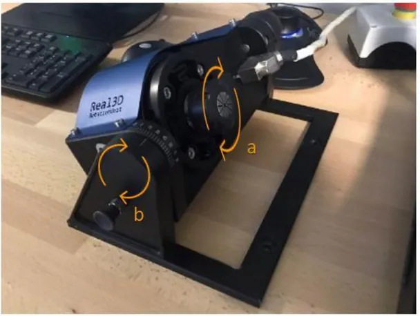
Finally, the Real 3D rotation unit mentioned above is an easy way to solve the problem of undercuts and to obtain complete solid representations of tools and micro-tools. In few words, it is a rotation unit that must be fixed on the xy plane and that is constituted by a motorized rotational axis, at which the tool is fixed, and a manual inclination axis that allows to tilt the inspected object with respect the xy plane.

The complete three-dimensional representation of tools is obtained by rotating the tool itself by 360° (at discretized steps) along its principal axis and by applying the same acquisition principles explained above to each angular position.

After all data have been acquired, points collected are merged and a triangle mesh is defined to obtain the final representation of the tool.

It should be noticed that to obtain a complete representation of the tool along its body the xy reference plane must be moved in order to acquire different data along the axis of the tool.

Figure 2.2.1-3 - Real 3D rotation unit for tools inspection. a) motorized rotation axis; b) manual tilt axis

2.2.2 Algorithms for focus definition

As previously explained, FV microscopy works by vertically scanning a surface within a z-range.

When images in vertical direction are stored, the purpose is to associate to each pixel of the images an index able to characterize if it is in focus or not. Unfortunately, it is impossible to do so by considering only a single pixel without accounting the neighbor ones.

Therefore, in order to compute this operation, a small patch of pixels around the considered one must be taken into account. This procedure represents one of the greatest limitations of the focus variation technique because it leads to a significant reduction of the maximum lateral resolution achievable.

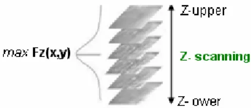
Deeply in detail, the detection of the surface of the part is obtained by calculating the maximum focus variation value within the scan range. [38]

A measure of focalization can be computed on a square n x n of pixels, for every image

Iz and for every point with coordinates (x, y) belonging to that image. Its expression is the following one:

𝐹_𝑧(𝑥, 𝑦) =

√∑𝑖∈𝑟𝑒𝑔𝑤(𝐼𝑧(𝑥,𝑦))(𝐺𝑉𝑖 − 𝐺𝑉̅̅̅̅)2

𝑛

where GVi is the grey-value of the i-th pixel, 𝐺𝑉̅̅̅̅ is the average grey-value of regw(Iz(x,y))

and n is the number of involved pixels.

Thus, for every point a curve of focus information is fitted containing information (about focalization) of every z-position of the scanned surface. Therefore, finding the maximum of each curve means finding the z-height of each point constituting the inspected surface.

In order to summarize and to better understand the procedure, it can be said that the microscopy system stores images of the specimen at different z positions (defined by the vertical resolution), computes the index function Fz for each pixel at each level, fits

the curve of focus information and finds its maximum.

Figure 2.2.2-1 - Focus-variation working principle and maximum value of the focalization function. [38]

The maximum value found corresponds to the height at which the considered point is in focus. In this manner, it is possible to reconstruct the 3D representation of the object merging all points collected with their height (deriving from previous steps) and color information.

Thanks to this explanation, it is easy to understand why step surfaces are of difficult interpretation for FV algorithms.

In fact, in correspondence of these kinds of surfaces, the Fz function can exhibit more

than one peak or can have its maximum at a non-correct position. This phenomenon is due to the fact that some pixels of this specific region are in focus at a certain height, but nearby pixels could be in focus at a very different height because they belong to a completely different surface (Figure 2.2.2-2).

Figure 2.2.2-2 - Schematic representation of the information curve used to reconstruct the three-dimensional surface of a specimen with a step height.

2.3 State of the art of dental bone drilling

This specific paragraph is of fundamental importance to provide a solid knowledge on the state of art of bone drilling (more precisely, dental bone drilling).

2.3.1 Problem statement

Drilling operations in dentistry, as opposed to other mechanical processes, face several problems strictly related to the organic nature of the work material. Particularly the temperatures generated during the operation must be kept below a specific threshold, commonly identified as 47 °𝐶[44]_{. This threshold can be only}

exceeded for a very short amount of time, around one minute, before the bone suffers from thermal damage, specifically osteonecrosis.

Along with the process parameters, one of the main causes of the thermal gradient is the wear of the drilling tool.

The most important thing that must be taken into account is the variability in working parameters adopted during the operations. As it can be easily understood, the huge problem in this field is the fact that the main driving force behind the choice of the parameters is the personal experience of the dentist.

This must be summed to the fact that the tool is usually held by the dentist himself, therefore each operation would be clearly completely different from the other ones. The success of dental implants depends on many factors, one of which is the capability of the drilled bone tissue to heal around the implant and integrate it. To facilitate the process, it is imperative to minimize the damage to the tissue, particularly by making sure the heat generated does not cause a thermal injury, resulting in osteonecrosis. During the drilling operation most of the mechanical energy is turned into heat, focused at the drilling site. The heat influences not only the drill bit and the bone but the chips as well. Because of the narrow drilling area, the heat dissipation can be intense. This dissipation is made even harder by the inhomogeneity of the bone and its anisotropic thermal properties.

Thermal osteonecrosis is suggested to be generated not only by the friction with the tool, but also by mechanical vibrations [39] _{and by the possibly of damage to blood}

vessels, that reduces blood flow and heat dissipation.

Bone drilling studies play a critical role in improving the chances of avoiding thermal osteonecrosis. [14] [24] [41] [42]

Many significant parameters affecting bone drilling have been identified, but so far, no general agreement was achieved among the scientific community regarding many of these factors, such as drill design or drilling speed.

An example of this, is given in Chapter 1.3 when explaining geometric features of drills for bone applications.

2.3.2 Temperature threshold

Many studies have been focused on identifying the temperature threshold and the maximum amount of time the bone tissue can actually bear it before incurring in necrosis.

It must be taken into account that lots of investigations were performed on animal bones, which are microscopically different from human one. Therefore, the exact threshold temperature can only be approximated.

In 1972 Matthews and Hirsch [43] _{noted that, when no proper cooling strategy was}

adopted, temperatures around 100 °C were easily reached. Furthermore, they found that the force applied to the drill was a much more significant factor than the drilling speed in both magnitude and duration of the temperature increase. Particularly it was recorded that at increasing force the maximum temperature and its duration decreased.

Further investigations made by Eriksson et. al. [44] _{established the limit temperature to}

be 47°C and the maximum drilling time of 1 minute.

2.3.3 Mechanical parameters

Aldabagh [45] _{performed a research with drilling speeds close to literature ones}

(between 1250 and 2500 𝑟𝑝𝑚). Results showed that high drilling speeds lead to a reduced maximum temperature achieved by bone tissue and, in parallel, also to reduced time at which the temperature itself is at its maximum value. The reason is probably related to the fact that the time required to finish the operations lowers. Maximum temperature evaluated in this study are of 40°𝐶 for the 2500 𝑟𝑝𝑚 speed. It should be noted that in this experimentation campaign an external cooling system was adopted.

Regarding the drilling force, an increasing load is linked to two main phenomena. If the applied force is increased the drilling time is reduced and so the duration of the temperature increase, and the final maximum temperature decrease too. At the same time, the friction between drill and bone is increased, causing a rise in the instantaneous heat generation. Therefore, an optimum value for the drilling force must be found, in order to achieve an ideal trade-off between these two opposite effects. Toews et. al. [44]_{, instead, recorded the effects of feed rate for low drilling speeds.}

At increasing drilling speed, the temperature increased as well. Increasing the feed rate, on the other hand, lead to a decrease in the maximum temperature.

Generally speaking, it is possible to reduce the effect of large diameters by pre-drilling with a smaller drill bit. This procedure obviously increases the operative time.

2.3.4 Tool wear monitoration

Under the point of view of drill wear monitoring and inspection, Clement et. al.

[47] _{studied the effect of different feeding forces and spindle speeds on four different}

kind of drill bits for bone applications.

Surfaces of bits were directly analysed using common magnification microscopes and scanning electron microscope (SEM).

The limitation of this approach is represented by the fact that images acquired were evaluated only under a subjective point of view. In fact, the quantification of the state of wear was carried out by filling tables with subjective opinions (like for example “moderate breakouts”, “surface finish slightly rough” etc.) driven by visual inspection of the worn surface of the tool.

However, it should be said that the principal aim of the paper was not concerned in evaluating methods for tool wear inspection but, rather, in studying performances of different drill bit geometries and materials in order to suggest to specialists (dentists, surgeons etc.) the best solution to adopt.

3

Chapter 3

DATA COLLECTING: PROCEDURE AND MATERIAL

It is necessary to spend some words in the definition of the procedure and methods adopted for the acquisition of data.

As mentioned in previous chapters, developed algorithms will be validated by applying them to a real experimental problem. Therefore, from now on, images and reasoning will be referred to this specific case for the sake of simplicity and to better understand the logic behind algorithms.

What is important, instead, it is to understand the set-up implemented for acquiring data of drill bits to be analysed and the preliminary results that can be obtained by using Alicona Measuring Suite and CloudCompare v2.6.3 (CC)[50] _software.

The procedure adopted is the following one:

1. Three-dimensional acquisition of the new tool by means of the Alicona Infinite

Focus measuring device equipped with the Real 3D rotation unit.

The tool is represented by a dental drill bit AISI 420B of diameter Ø 2.3 mm. The bit is covered with a layer of DLC (Diamond-like carbon) of thickness 0.5-3 µm.

2. Utilization of the tool in the experimental campaign. 3. Acquisition of the cloud of points of the worn tool. 4. Preliminary results with Alicona Measuring Suite. 5. Preliminary results with CloudCompare v.2.6.3.

6. Elaboration and manipulation of the two acquired clouds of points with developed algorithms in order to obtain detailed numerical results.

It should be noticed that the Alicona Infinite Focus system is a micro-metrology tool device exploiting the focus variation measuring principle explained in Chapter 2.2.

Figure 3.1 - Alicona Infinite Focus measuring device equipped with the Real 3D rotation unit.

3.1 Acquisition parameters

Before starting the acquisition, different parameters must be set in order to obtain reliable and repeatable measurements.

Below, some of the most important parameters are explained.

• The exposure is the amount of light per unit area reaching an electronic image sensor.

In acquisitions with FV it is an important parameter to be set because it influences the amount of light hitting the inspected surface. Exceeding with the exposure value could increase the risk of reflections from the inspected surface. Vice-versa, decreasing its value can lead to some problems in illuminating it correctly.

Therefore, when setting its value, the surface reflectivity of the object must be taken into account.

• The contrast is the difference in colour and tone that contributes to the visual effect of an image.

Usually, when dealing with 3D acquisition of tools it is set to a value of 0.3. • The vertical resolution is the capability of the objective lens to discriminate

two adjacent features (or points) along the vertical z-axis.

In other words, it is the minimum distance (along the z direction) between two adjacent points that can be detected by the optic system.

As mentioned, when explaining the working principle of FV, it is one of the most important parameters because it determines the number of vertical scans and, consequently, the capability of acquiring a large variety of surfaces and slopes. • The lateral resolution, in the same way of the vertical one, is the capability of

the objective lens to discriminate two adjacent features along the transversal direction with respect to the optical axis.

Due to algorithms governing the focus variation system (explained in Chapter

2.2), lateral resolution achievable is not as good as the vertical one.

• Radius upper and Radius lower are respectively the upper and lower vertical bounds within which the acquisition must be carried out. Their value depends, in this specific case, on the dimension of the drill bit radius.

• The axial measurement is an option that can be set to obtain a complete measurement of the tool along its axis.

In fact, the dimension of one single image (along the axis of the bit) acquired by the system could not be sufficient to cover the whole portion of the tool the researcher is interested in. Therefore, by setting approximatively the value of the axial measurement (in millimetres), the system will acquire different images/data along the principal axis of the tool (following the same rules explained in Chapter 2.2) and can reconstruct its whole geometry.

Table 3.1.1 - Example of measurement parameters.

In Figure 3.1.1 an example of parameters used for data acquisition of the drills mentioned above is shown.

It should be noticed that acquisitions of these specific drills for dental bone application lasted about 5 hours for an axial measurement distance of 3.49 mm.

Results obtained are saved in files with STL extension [51] _{and, after preliminary}

analyses with the Alicona measuring suite, are exported to secondary devices (e.g. personal computers) to compute further examinations.

The STL acronym stands for STereoLitography and represents one of the most diffused file formats born for stereolitography CAD software.

This particular kind of file is used for the 3D representation of objects by means a triangulation of a points cloud with three-dimensional surfaces, like for example triangles (called faces).

Deeply in detail, an STL file is represented by two matrices. The first one is an n x 3 matrix containing the xyz coordinates of the vertices constituting each triangle (n is the total number of points). The second one, instead, is an m x 3 matrix containing the normal vectors (in rows) of each surface composing the three-dimensional object (m is the total number of faces or triangles).

Figure 3.1.1 - Example of an STL file of the examined drill bit for dental bone application.

3.2 Specimen material

These samples were provided by the BIOMEC Company. It is pertinent to mention here that the samples were dry (free from blood) and degenetized. Specifically, these samples were taken from portion of leg and then processed.

As shown in Figure 3.2-1 and Figure 3.2-2, we can see that there are two portions, starting from the top cortical (harder) and beneath it the other one trabecular/Cancellous (softer). Overall the bone sample is not perfectly homogenous which makes it close to the reality.

We had 200 samples of equine bones of each sample of size 30*30*17 mm. Not all of the samples have uniform thickness of the cortical section.

The first objective was to separate the samples based on the uniformity of the cortical thickness. At the end we sorted out 72 samples dedicated to real campaign of experimentation with an average thickness of the cortical section above 3mm.

3.3 Drill bits used for tests

We had three tools provided by the Biomec company with the coating on the surface of it. Coating was done before the execution of the experimentation because by doing that we can possibly avoid wear up to some extent, protect it from external environment and helps in making compatible biologically. These drill bit replicate the same conditions as they were supposed to be used in real standard dental procedure. Going into details about the drill bits we had were about the diameter 2.3mm and its length equal to 15mm.

Figure 3.3 – 3 Drill bits used for tests.

4

Chapter 4

Experimental set up

For the experience, specific dentistry equipment is adopted in order to improve the realism of the experiment. The experimental apparatus presented here are only a small part of a larger experimental campaign undertaken by Politecnico di Milano in the field of dental bone applications research.

In particular, the work explained below is only a resume (focalized only on 3D analysis of wear) of the larger experimentation developed in collaboration with another graduating student. Therefore, wider explanations and more exhaustive considerations about this topic are provided in the master work thesis of the colleague mentioned above [49]_.

4.1 Experimental apparatus

Here, a list of the experimental apparatus is exposed.

• iChiropro specific dentistry contra angle CA 20:1 micro-series (Bien Air). • iChiropro micromotor MX-i LED (Bien Air).

• iChiropro iPad software system application (Bien Air). • 3 axis machine opportunely modified to execute tests. • Dynamometer Type 9317B (Kistler).

• Torque meter Type 9329A (Kistler). • Cooling water system.

• Water collection tank

It should be noticed that devices like the dynamometer and the torque meter are utilized for specific analyses developed in the master work thesis mentioned above.

4.1.1 Dentistry equipment

In order to improve the realism of the experiment, specific dentistry equipment was adopted, in particular an actual dentistry set called the iChiropro system (Bien-Air).

Figure 4.1.1 iChiropro, Contra-angle and MX-i LED micromotor (Bien-Air) The whole system is controlled by the associated iPad application, which allows the dentist to set, monitor and regulate the main parameters of the surgical operation: torque and rotation speed generated by the micromotor, the flow rate of the cooling system and the lighting of the drilling zone.

The micromotor is the MX-i LED in which the power is regulated and stabilized by the electronic system that allows the speed to be maintained with great precision during the operations. The power is transmitted to the contra-angle CA 20:1 L

micro-series. This component allows to transfer the torque to the drill bit. It is equipped by

internal irrigation system in which the physiological liquid flows. After, the latter come out by the nozzle providing an optimum irrigation both the drill and working zone. Micromotor and contra-angle constitute the instrument called “mandrel” by dentists.

Table 4.1.1 Micromotor and contra-angle data

MX-i LED Micromotor CA 20:1 L contra-angle

Torque [Ncm] 6.8 70

4.1.2 Machine

CNC 3 axis machine (Figure 4.1.2-1) characterized by working volume of 130x90x40 mm3 _{was selected for this work.}

Figure 4.1.2-1 CNC 3 axis machine

The machine is moved by three stepper motors, one for each axis. For the movement in the x and y direction, the motors were two phase stepper motors 42HS34 – 1304A. For the z direction, it was a two phase JK42HS34-1334. Table 4.1.2 shows specification of stepper motors that used in machine.

Table 4.1.2 Stepper motors datasheet

42HS34-1304A JK42HS34-1334

Holding torque [Ncm] 28 21.5

Step angle [°] 1.8

Voltage [V] 3.2

The motors are connected to an EleksMaker board (Figure 4.1.2-2), powered at 12 V and 5 A. The controller board translates the commands coming from the pc, to which it is connected through a USB port.

Figure 4.1.2-2 EleksMaker board

The machine is moved by inputting a set of commands written in G-code, which is the language the machine uses to operate.

4.2 Fixture preparation

For the placement of the given equine samples rigidly, we used aluminium block. And we drilled four threaded holes on two sides (opposite to each other). By doing so, we can hold sample at place and avoide any type of displacement during operational time.

4.3 Realization of horizontal configuration

We need two different setups, to drill hole in vertical and horizontal direction. These two setups are utilized for specific analyses developed in the master work thesis mentioned above [49]_.

To ensure the horizontal direction of the spindle some changes were inevitable in the dentistry equipment support. That task was done by maintaining the static strength of the spindle at the same time because slight vibrations during process can jeopardize the whole task. Another aspect to consider while making those necessary changings were not to increase the weight of support as whole too much (it must remain in acceptable limits).

Figure 4.3 – spindle held together with mandrel by means of NEW fixture

As shown in the Figure 4.3, horizontal configuration was achieved by adding one more fixture which was attached to the dentistry equipment support. That fixture made possible the direction of the spindle exactly parallel respect to the equine sample.