Building and Architectural Engineering
Track - Building Engineering
A PARAMETRIC DESIGN WORKFLOW APPLIED TO A RESPONSIVE
CURTAIN WALL SYSTEM FOR DAYLIGHT OPTIMISATION OF AN
EXISTING BUILDING
Supervisors:
prof. Gabriele Masera
prof. Simone Giostra
Thesis work by:
Pietro Pavesi
854515
3
Table of contents
1 THESIS TOPICS ORIGINS ... 20
1.1 Circadian rhythm ... 22 2 CONCEPT ... 25 2.1 Introduction ... 25 2.1.1 Case studies ... 27 2.1.2 Analyses procedure ... 30 3 ANALYSES METHOD ... 35 3.1 Introduction ... 35
3.2 Daylight performance metrics ... 35
3.2.1 Daylight Factor ... 36 3.2.2 Dynamic metrics ... 36 3.2.3 Metrics choice ... 38 3.2.4 Software choice ... 39 3.3 Inputs ... 40 3.4 Façade dimensions ... 41 3.5 Destination of use ... 41 3.6 Elements Properties ... 42 3.6.1 Analyses grid ... 43 3.7 Project location ... 43 3.7.1 Surrounding Context ... 45 3.8 Orientation ... 47 3.9 Analysis period ... 47 3.10 Schedules ... 47 4 CASE STUDIES ... 51 4.1 South-facing modules ... 51 4.1.1 CASE 1 ... 53 4.1.2 CASE 2 ... 60
4 4.1.3 CASE 3 ... 69 4.2 West/East-facing modules ... 78 4.2.1 CASE 1 ... 80 4.2.2 CASE 2 ... 83 4.2.3 CASE 4 ... 88 4.3 Comparisons ... 94
4.3.1 Comfortable configurations percentage ... 95
4.3.2 PV panels incident radiation ... 100
4.4 Facade tiling... 101
4.4.1 Same-shape façade modules ... 102
4.4.2 Different-shape façade modules ... 103
4.4.3 CASE STUDIES ... 104
4.5 Modules dimensions halving ... 109
4.5.1 South-facing modules ... 112 4.5.2 West-facing modules ... 115 5 RE-CLADDING ... 118 5.1 Context description ... 119 5.2 Re-cladding strategies ... 123 5.3 Environmental analyses ... 126 5.3.1 Shadows Analyses ... 126 5.3.2 Incident Radiation... 128
5.4 Simulation model set-up ... 129
5.4.1 Thermal model... 129 5.4.2 Daylight Model... 132 5.5 BASELINE CASE ... 135 5.5.1 Daylight ... 135 5.6 CASE STUDY ... 138 5.6.1 Optimization process ... 139 5.6.2 Galapagos options ... 140 5.6.3 Final configuration ... 141 5.6.4 Daylight results ... 142
5 5.6.5 Geometrical results ... 145 5.6.6 PV panels efficiency ... 148 5.6.7 Energy demand ... 151 6 CONCLUSIONS ... 154 6.1 Economical aspect ... 154 6.2 Digital deepening ... 154 6.3 Architectural aspect ... 155 7 APPENDIX A ... 157 7.1 Introduction ... 157 7.1.1 General Legend ... 157
7.2 DIVA for Rhino ... 158
7.2.1 Rhino modeling ... 158 7.2.2 Grasshopper modeling ... 159 7.2.3 Rhino+Grasshopper modeling ... 160 7.3 DIVA workflow ... 161 7.3.1 Sun Diagram ... 161 7.3.2 Daylight Simulation ... 162 7.3.3 Results Visualization ... 169
7.3.4 Incident Solar Radiation ... 172
7.3.5 Radiance Visualization ... 173
8 APPENDIX B... 179
8.1 Thermal zone ... 179
8.2 Glazing elements ... 183
6
List of figures
Figure 1.1 – Melatonin daily levels ... 22
Figure 1.2 – Sensitivity curves ... 23
Figure 2.1 - Ideal automatic form-finding process ... 26
Figure 2.2 - Facade starting box ... 27
Figure 2.3 – CASE 1, geometrical introduction ... 28
Figure 2.4 – CASE 2, geometrical introduction ... 29
Figure 2.5 - CASE 3, geometrical introduction ... 29
Figure 2.6 - CASE 4, geometrical introduction ... 30
Figure 3.1 - Facade materials variety ... 42
Figure 3.2 - Analyses grid description ... 43
Figure 3.3 - Adjacent facade modules ... 46
Figure 3.4 - Volume examples to be possibly re-cladded ... 46
Figure 4.1 - Elements properties ... 53
Figure 4.2 - Schematic vertical section ... 53
Figure 4.3 - Constant PV length sub-cases ... 54
Figure 4.4 - Constant angle sub-cases ... 55
Figure 4.5 - Geometrical evolution ... 60
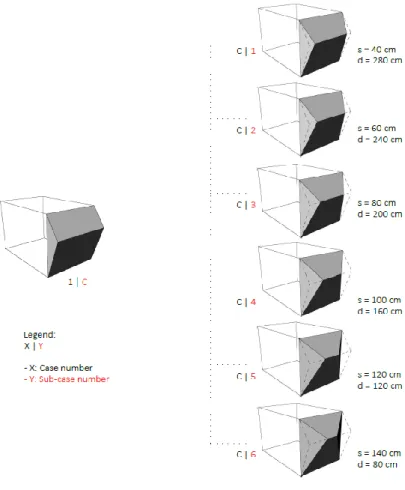
Figure 4.6 - Elements properties ... 61
Figure 4.7 - Variables within CASE 2 sub-cases ... 62
Figure 4.8 - “C” family ... 63
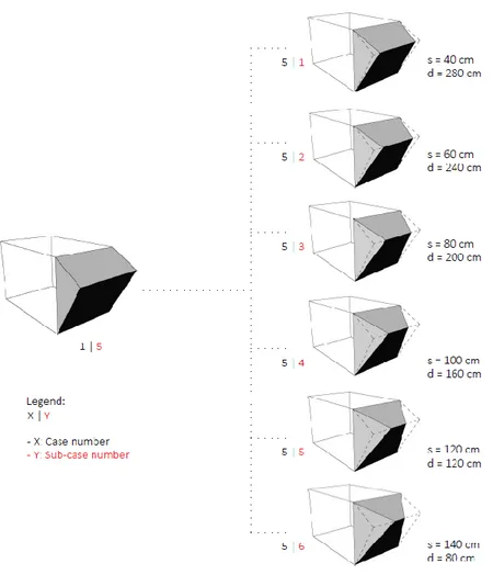
Figure 4.9 - “5” family ... 64
Figure 4.10 - Elements properties ... 69
Figure 4.11 - Horizontal section of the Case 3 geometry ... 69
Figure 4.12 - Sub-cases matrix ... 70
Figure 4.13 - Perspective view, opaque panels subject to analysis ... 71
Figure 4.14 - Schematic top view ... 71
Figure 4.15 - Schematic top view ... 73
Figure 4.16 - Elements properties ... 80
Figure 4.17 - Elements properties ... 83
Figure 4.18 - Sub-cases configurations ... 83
Figure 4.19 - Sub-cases configurations ... 84
Figure 4.20 - CASE 2 technological variation ... 84
Figure 4.21 - Elements properties ... 88
Figure 4.22 - Horizontal section of the Case 4 geometry ... 88
Figure 4.23 - Sub-cases configurations ... 89
Figure 4.24 - Sub-cases configurations ... 92
Figure 4.25 - Procedure ... 94
Figure 4.26 - Comfort zone redefinition ... 96
7
Figure 4.28 - Control points representation ... 102
Figure 4.29 - Interferences detection... 102
Figure 4.30 - Interferences detection... 103
Figure 4.31 - Facades under investigation ... 105
Figure 4.32 - Vertical replicability ... 106
Figure 4.33 - Horizontal replicability... 107
Figure 4.34 - Façade transformation ... 109
Figure 4.35 - Original CASE 2 façade modules ... 110
Figure 4.36 - Halved CASE 2 façade modules ... 110
Figure 4.37 - Façade transformation ... 110
Figure 4.38 - Façade’s main parameters ... 111
Figure 4.39 - Analysis cases matrix ... 112
Figure 4.40 - 2 glazing panels are needed when West-faced ... 115
Figure 5.1 - Urban context ... 119
Figure 5.2 - Vertical longitudinal section ... 120
Figure 5.3 - BUI-12 breakdown ... 121
Figure 5.4 - Vertical section ... 122
Figure 5.5 - BUI-12 and obstructions ... 123
Figure 5.6 - Facade elevations ... 124
Figure 5.7 - Recessed curtain wall modules ... 125
Figure 5.8 - BASELINE curtain wall ... 125
Figure 5.9 - CASE STUDY curtain wall ... 125
Figure 5.10 - Facade modules dimensions ... 126
Figure 5.11 - Equinoxes – 20th March, 22nd September ... 127
Figure 5.12 - Summer Solstice – 21st June ... 127
Figure 5.13 - Winter Solstice – 21st December ... 127
Figure 5.14 - IR on North and East facades ... 128
Figure 5.15 - IR on South and West facades ... 129
Figure 5.16 - Typical floor plan ... 130
Figure 5.17 - Analyses for each zone ... 134
Figure 5.18 - Glare evaluation at the typical floor ... 138
Figure 5.19 - Re-cladding strategies ... 139
Figure 5.20 - Variable parameters ... 140
Figure 5.21 - Customized facade modules ... 141
Figure 5.22 - Optimized BUI-12 configuration ... 142
Figure 5.23 - Glare evaluation at the typical floor ... 144
Figure 5.24 - sDA and ASE values ... 145
Figure 5.25 - Vertical gradient trend ... 146
Figure 5.26 - Horizontal gradient trend ... 147
Figure 5.27 - Variable parameters changes ... 148
8
Figure 5.29 - IR on South and West facades ... 149
Figure 7.1 - Option A, Toolbar ... 157
Figure 7.2 - Option B, Typing a keyword ... 157
Figure 7.3 - Thermal zone modeled in Rhinoceros ... 158
Figure 7.4 - DIVA toolbar in Rhinoceros ... 159
Figure 7.5 - Parametric overhang system ... 159
Figure 7.6 - Possible integration within different tools ... 160
Figure 7.7 - Cooperation Rhino/Grasshopper... 161
Figure 7.8 - Scene Object focus ... 163
Figure 7.9 – Workflow ... 164
Figure 7.10 - Window set up ... 165
Figure 7.11 - Window component ... 165
Figure 7.12 - Grid definition ... 166
Figure 7.13 - Annual daylight component ... 167
Figure 7.14 - Workflow ... 168
Figure 7.15 - Daylight Factor ... 169
Figure 7.16 - Radiation ... 169
Figure 7.17 - Results visulaization ... 169
Figure 7.18 - Grid viewer component ... 172
Figure 7.19 - Workflow ... 173
Figure 7.20 - Visualization component ... 174
Figure 7.21 - Camera component ... 174
Figure 7.22 - Rhino viewport ... 175
Figure 7.23 - Sky component ... 176
Figure 7.24 - Workflow ... 176
Figure 7.25 - Rendering options ... 177
Figure 8.1 - Thermal zone... 179
Figure 8.2 - Thermal zone settings... 180
Figure 8.3 - Window component ... 180
Figure 8.4 - Window settings ... 181
Figure 8.5 - Workflow ... 182
Figure 8.6 - Workflow for planarity checking ... 183
Figure 8.7 - Wrong vs. right configuration ... 184
Figure 8.8 - Wrong vs. right configuration ... 184
Figure 8.9 - Focus on Window component ... 185
Figure 8.10 - Wrong vs. right configuration ... 185
Figure 8.11 - Schematic window decomposition ... 186
Figure 8.12 - Outputs list interface ... 187
9
List of tables
Table 3.1 - Recommended illuminance values ... 37
Table 3.2 - Radiance parameters ... 39
Table 3.3 - Office schedule ... 47
Table 3.4 - Residential schedule ... 48
Table 4.1 - IR comparison ... 72
Table 4.2 - IR comparison ... 73
10
List of graphs
Graph 3.1 - sDA-ASE-IR results ... 40
Graph 3.2 - Schedules comparison ... 49
Graph 4.1 - sDA-ASE-IR results ... 56
Graph 4.2 - Results trend ... 57
Graph 4.3 - sDA-ASE-IR results ... 58
Graph 4.4 - Recalling CASE 1 results ... 62
Graph 4.5 - sDA-ASE-IR results ... 64
Graph 4.6 - sDA-ASE-IR results ... 65
Graph 4.7 - Recalling CASE 1 results ... 66
Graph 4.8 - sDA-ASE-IR results ... 67
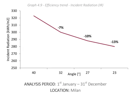
Graph 4.9 - Efficiency trend - Incident Radiation (IR) ... 72
Graph 4.10 - Efficiency trend - Incident Radiation (IR) ... 73
Graph 4.11 - Efficiency trends comparisons ... 74
Graph 4.12 - sDA-ASE-IR results ... 75
Graph 4.13 - sDA-ASE-IR results ... 76
Graph 4.14 - Results comparison ... 77
Graph 4.15 - sDA-ASE-IR results ... 81
Graph 4.16 - sDA-ASE-IR results ... 85
Graph 4.17 - Results trend ... 86
Graph 4.18 - sDA-ASE-IR results ... 91
Graph 4.19 - sDA-ASE-IR results ... 93
Graph 4.20 - sDA-ASE-IR results ... 93
Graph 4.21 - South exposure, cases comparison ... 95
Graph 4.22 - South exposure, cases comparison ... 97
Graph 4.23 - West exposure, cases comparison ... 98
Graph 4.24 - West exposure, cases comparison ... 99
Graph 4.25 - South exposure, IR values ... 100
Graph 4.26 - West exposure, cases comparison ... 101
Graph 4.27 - South exposure, cases comparison ... 113
Graph 4.28 - South exposure, cases comparison ... 114
Graph 4.29 - West exposure, cases comparison ... 115
Graph 4.30 - West exposure, cases comparison ... 116
Graph 5.1 - sDA-ASE results ... 136
Graph 5.2 - sDA-ASE results ... 143
Graph 5.3 - Total useful PV area ... 150
Graph 5.4 - Energy production according to the orientation ... 151
Graph 5.5 - Ideal heating&cooling demand ... 152
11
ABSTRACT
The thesis work represents a research which explores different aspects of a typical early-design process of building envelopes. The work discusses the definition of a parametric workflow, to be easily and fluently repeated to any kind of newly-constructed or refurbished project, which goal is an energy efficiency-based form-finding. The indoor visual comfort, paired with the energy production within the façade-integrated photovoltaic panels, plays the role of driving force in order to create optimized and customized façade systems. The first part of the work is based on the familiarization with the simulation digital tools, while the last part on a re-cladding exercise, where the building envelope is highly optimized according to the site boundary conditions. The work has shown promising results on the energy efficiency point of view, achieved by means of the folded curtain walling façade modules.
KEYWORDS
Daylight simulations, parametric modeling, Grasshopper, DIVA, folded surfaces, optimization, spatial daylight autonomy, annual sunlight exposure, BIPV, Building Integrated Photovoltaic, re-cladding, building envelope, responsive facades
13
ACKNOWLEDGMENTS
Acknowledgments go to both the supervisors, prof. G. Masera and prof. S. Giostra, for their assistance and support since this thesis work began in March. I am very grateful for their contribution, their helpful ideas, suggestions and for making this long trip an inspiring and promising work within the parametric modeling, the façade and the daylight world. I express my deepest gratitude for their appreciations of the whole research work, which has been morally the driving force.
I extend thanks to prof. M. Pesenti, for having introduced me to the daylight simulations world, and for his support within the simulations whenever was needed.
15
INTRODUCTION
The thesis work has been a journey into the daylighting simulations world, by means of the so-called DIVA for Rhino software; it was unfamiliar to me when, on the early April, I started moving the very first steps of this research work. By exploiting this lack of knowledge about the software needed for the analyses, this research could be considered a parallel path between the understanding of the software’s options and properties and the modeling phase. For these reasons, a detailed guide of this software has been included within the Appendixes. Consequently, my intent has been providing the readers - most of them may be architects, engineers or students as well – a large know-how of the main daylight-related-metrics and the awareness of the daylight-based design within the building skin.
17
NOMENCLATURE
Magnitudes
ASE Annual Sunlight Exposure [%] sDA Spatial Daylight Autonomy [%] DA Daylight Autonomy [%] DF Daylight Factor [-] UDI Useful Daylight Illuminance [%]
E Illuminance [lux] IR Incident solar Radiation [kWh]
[kWh/m2]
Acronyms
NZEB Nearly Zero Energy Building DHW Domestic Hot Water
BIPV Building Integrated Photovoltaic
AEC Architecture, Engineering and Construction PV Photovoltaic
19
1
THESIS TOPICS ORIGINS
20
1 THESIS TOPICS ORIGINS
This research work finds its bases on some common interests of the supervisors and me within the AEC field. The key words which may summarize at its best this thesis are “daylighting”, “curtain walling” and “parametric design”. They are also the aspects I have really enjoyed the most during this 2 year at Master of Science Degree; this research has been a very challenging path followed by inspiring professors, and hopefully the knowledge I acquired these months will represent a solid basis for my future career. It is my great pleasure to explain the origins of these 3 topics within the Master courses.
- daylighting: it is the last one in a chronological sequence which came to me, but it is the very first one for this thesis: it is actually a subject which is not widely thought in the universities, but it plays to me a fundamental role within the design process of any building; - curtain walling: it is for sure the most fascinating topic according to my personal interest; I
have the pleasure to live in a city which is under renovation and refurbishments, and often they are coupled with curtain walling technologies. There is no doubt glazing facades fascinate most of the people, both experts of AEC field and the rest of them, and I have always had the will to study a curtain walling aspect during the thesis work;
- parametric design tools: differently from the previous inputs, this is a the technological tool which is largely growing these years between the AEC community; it is actually represented by any software which ensures the user a parametric control of any project parameters. Within my thesis, it has the function to melt the previous inputs in such a way they could communicate and affect each others: basically, the daylighting results will influence the façade geometry.
The previous 3 topics concern different aspect of a project: the daylighting represents the environmental parameter, the curtain walling covers the architectural aspect, while the parametric tools represent the computer-based modeling phase. They may be also perfectly matched together and collaborate in order to solve the thesis issue, which is the façade form finding based on the daylight comfort of the occupants. In fact, daylighting finds its maximum expression in curtain
21
walling-covered buildings, since their almost-100% glazing surface allows the light penetrating the internal spaces. Of course this is not only a positive aspect, since a large glazing percentage on a building façade may represents also a high risk of glare and overheating within the internal environment. All these pros and cons, and many others will raise in the next pages, are the main inputs of the thesis; they have to be faced, managed and solved in such a way the comfort must be ensured for the clients and occupants. So, the daylighting topic was matched with the building façade one, and finally implemented with the parametric design tool; the “marriage” between these aspects gives birth to the research work you are going to read in the next chapters.
The next paragrph§1.1 is focused on a short introduction about the importance of natural light in the everyday life, exploring the scientific aspects behind it.
22
1.1 Circadian rhythm
The very first step I did, while approaching for the first time to the “natural light world” has been learning the importance of light in the people’s life. Actually, I could have understood that from around the beginning of the XXI century, scientists have discovered new relationships between the health and the availability of the light. The main document I have used to get information was the paper sponsored by ENEA “Studio per la valutazione degli effetti della luce sugli esseri umani” by M. Barbalace, F. Gugliermetti, F. Lucchese, F. Bisegna.
In the 2002, in fact, a new photoreceptor inside the retina was discovered (called MELANOPSIN), and it is considered as the main “actor” for the regulation of the biological clock. That research has cleared and confirmed the relationship between light and our biological rhythms, the so called circadian rhythm.
The circadian rhythm is basically the sleep/wake cycle of a person, and it is regulated by several functions.
Light is the main one, but it is coupled with other elements such as the time of the meals, the sound, temperature, social interactions and caffeine. Anyway, light is the principal one since it modifies the amount of Melatonin in our blood.
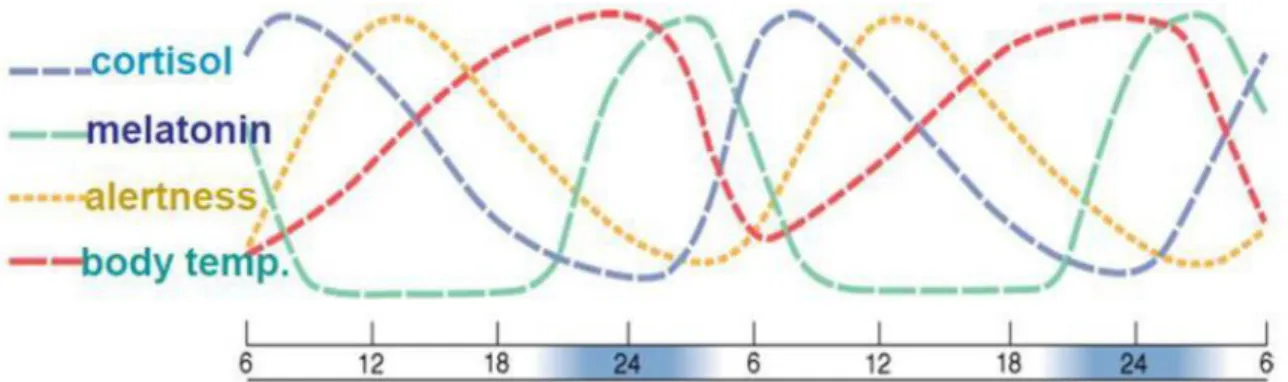
Figure 1.1 – Melatonin daily levels
As it can be seen by the picture above, the level of Melatonin typically increases during the night, having a peak at around 2.00-4.00 am, and then it tends to decrease reaching the minimum value in the hours of the day; so, the secretion of melatonin and the availability of light are inversely proportional. At this point is much clearer how the light influence our sleep/wake cycle and how it could shift the circadian rhythm.
Going a little bit more into details, it is known that referring to “light” is too generic; in particular, the elements which contribute to the shift of circadian rhythm are:
1. light quantity/type
23 3. time of application of a light source
4. direction of application of a light source
I will explore a bit more the first points 1 and 2 of the list above; actually the points 3 and 4 are pretty obvious.
As concerns the number 1, there are huge differences between an artificial light and the natural one in terms of lux availability. In fact, the lux of artificial lights in indoor environments are around 1000 lux, rarely above this threshold; while the amount of natural light hitting the ground in the worst conditions, under an overcast sky, varies within 2000-10000 lux. By comparing the two illuminance levels it is clear that the level in the indoor space are not enough to guarantee the right drop of the melatonin level.
As far as the point 2 is concerned, it can be described by the following picture, which shows different curves of sensitivity; we are interested in the two about the melatonin suppression:
Figure 1.2 – Sensitivity curves
By analyzing the graph, I can state that the maximum suppression of melatonin corresponds to the wavelength of about 460 nm, related to the region of “blue”. At these wavelengths, in fact, the eye is much more sensitive rather than the others. Those lights which are made up of short wavelengths (blue ones) are more powerful in terms of suppressing the melatonin.
As a conclusion, a good design of a building/space will have to include also the circadian component, since it has such a relevant role in our everyday life. This design issue will have to match also the requisites of sustainability and efficiency. Within this thesis work, the effort has been the implementation of the natural light component during a façade module design, enhancing the visual comfort level of the indoor spaces.
24
2
CONCEPT
25
2 CONCEPT
2.1 Introduction
Within this chapter, I will introduce the main characteristics which have affected the very initial stage of this research work, towards the paradigm definition.
As said at the previous chapter§1, the will of the thesis has been clear form the very beginning of the design: this will is represented by the perfect marriage between those topics I have mentioned at the previous chapter, such as the natural light-based design, the curtain walling elements and the computational digital tools. Their union plays the main role within this design process: in fact, the thesis work is focused on the development of a methodology, which could be applied and used within several different projects, for both the cladding and re-cladding of a building’s envelope. The methodology, or better called workflow, will be able to be applied onto any kind of building shape, and it will produce as the final output a certain façade module, which would be the most suitable for that project. We are going to see later which are the parameters to be considered when I mention that a façade module is “the most suitable for that project”.
Nowadays, every newly-designed or refurbished building has to comply with the national and international standards about the sustainability topic; the design’s aim of every project should be getting as much close as possible to a Nearly Zero Energy Building. That smart design procedure brings so many fundamental benefits, such as first of all the CO2 emissions reduction, but also a cost
saving for the tenants and a more comfortable feeling within the internal space.
So, even in this research work the final aim is the reduction of the total energy demand on a yearly basis; in order to achieve this goal, the main interest field is the building envelope, since it is that layer which separates the aggressive external conditions and the comfortable internal spaces. For this reason, the envelope is the very first aspect to be designed and to pay the attention on, when considering the energy efficiency of that building. It is responsible of the heat transfer between the outdoor and indoor spaces, on all the different points of view; the conductive heat transfer, the ventilation, and the solar gains.
So, after having stated all these boundary conditions within a smart design procedure, I can get back to the thesis purpose. The aim is the definition of an algorithm which may help designers during early-design stages in the form-finding process of the building skin. As said, the algorithm has to produce a façade geometry which is optimized for that specific project characteristics; as a consequence of this statement, it is clear as the workflow has to respond to different possible parameters, which are also the main ones to be considered during the early-design stage of a new project. These parameters are those which make every project different and peculiar with respect to the other ones: the project location, the building shape and orientation and the destination of use. These may be classified as the “building characteristics”; actually they are not the only parameters to be considered within the workflow I am going to build up in the next chapters of the
26
thesis work, since they are coupled with those parameters related to the building performances and sustainability.
Probably, the main environmental aspect which will be faced during this research work, is the sun. Actually sun is the source of two of the main magnitudes for a building; solar radiation and the natural light. The innovative aspect of this research is the way we want to get as much close as possible to the NZEB targets: in fact, the geometrical form-finding will be based on the optimization of the sun-related magnitudes, since they are strictly related to each other. On one side, the façade geometry will assume a shape that optimizes the visual comfort within the internal spaces and rooms, and on the other hand it will try to reduce as much as possible the overheating and glare risks. It is important to state from the very beginning the will of reaching those goals through the only geometry of the façade; for this reason no shading systems or internal blinds will be considered.
Finally, it is fair to clarify that the whole process I am going to explain within the next chapters, will be mainly based on the visual comfort within the internal rooms; by “visual comfort” it is meant the condition which guarantees a high level of illuminance within a certain room, brought by means of the natural light only. Hence, the effort will consist in the respect of the visual comfort requirements, since it affects the electricity consumption and the occupants comfort, as I have explained in the last chapter when talking about the natural light role in the people’s life.
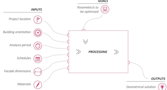
Hereby follows a preliminary scheme which stands at the basis of the work: it is utopian, if considered at the beginning of the thesis research, but it provides the reader an idea about the direction of my efforts during these period I have worked on that.
27
By analyzing the picture above, 4 main phases are identified: the inputs and goals settings, the information processing and finally the geometrical output. This very schematic representation helps to understand the degree of complexity and automation that must be faced before reaching a façade curtain walling shape, that fits the best a certain location, exposure, destination of use, by always ensuring the visual comfort for the occupants. Few words about the geometrical output should be spent; basically the possible façade shapes would be an infinite number, characterized by different numbers of surfaces, angles and materials. In order to simplify the problem solving, the number of possible outputs has been reduced. In fact, the thesis work will be limited to a particular family of geometries, which are all related to the same control points, as represented hereby by means of the perspective view.
.
Figure 2.2 - Facade starting box
By limiting the number of possible solutions as outputs of the automatic process, makes the first approach to the research easier, certainly. So, the next chapters are all focused on the analyses of those façade geometries which are generated by moving those control points, within the box that has been called “façade zone” (the pink-dashed-lines bounded space, in the picture above); please consider that the façade zone width is variable. The challenge of this research work will be the comprehension of the feasability of the process I have represented before: mainly, it will be curoius to understand the degree of automation that may be achieved. If results and final conclusions will be positive, the research will remain still open to any further implementation.
2.1.1 Case studies
Within this chapter the case studies will be introduced and described. They are only 4 possible geometries, deriving from the control points movement within the “façade zone”; they are generated by the control points shifting in the horizontal and/or vertical directions.
28
Basically, in the next few lines I’m going to introduce these 4 case studies which will be the starting point for the research work. They have quite different characteristics, due to their shapes, and for this reason will be interesting to test them in the next chapters, and see how they react to given boundary conditions.
It is important to state again, that the shapes you are going to see in the next paragraphs are taken only for an easy and proper comprehension, while their precise dimensions and characteristic will be described later; for this reason, the “façade zone” has been considered having a random thickness, in order to express the concept only. Same issue is valid for the “materials” properties; they will be treated later on, in order to assign in the best way the materials to every single façade surface.
Figure 2.3 – CASE 1, geometrical introduction
First case study is generated by bundling together couple of control points; point 1 is bundled with the number 3, and in the same way numbers 2 and 4. In such a way the geometry resulting from the control points manipulation is a sort of horizontal overhang.
29
Figure 2.4 – CASE 2, geometrical introduction
CASE 2 is the “child” of the previous geometry; the overhang is kept as in the CASE 1, and the two couples of control points are allowed to shift in the horizontal direction.
Figure 2.5 - CASE 3, geometrical introduction
The CASE 3 has a completely different configuration with respect to the previous categories. It has a vertical layout, with two lateral stripes and the central one. In order to make the analysis and simulations easier, the two stripes will be mirrored with respect to the central surface; in such a way they will have same area and same tilt angle.
30
Figure 2.6 - CASE 4, geometrical introduction
The last configuration represents an evolution of the CASE 3, or a 90°-rotation of the CASE 1. When we say evolution of the number 3, that means the control points have been coupled and it results at the end in only 2 points to be moved. Moreover, the two surfaces generated won’t have equal area, but all the possible variation will be later illustrated in the specific simulation chapter.
2.1.2 Analyses procedure
Once the 4 cases have been illustrated, it is convenient to introduce the way I am going to operate within the next chapters. By referring to the Fig.2.1, it is clear as one could not start a research by optimizing since the very beginning, since it is required to get in touch and acquire familiarity with the design tools and the whole set of parameters. For this reason, in the next chapters the reader will follow the path I have carried out during my research. The whole research is carried out by means of Grasshopper plug-in for Rhinocers; moreover, the analyses have been performed within two other plug-ins, completely suitable with Grasshopper, which are DIVA and ARCHSIM; these two are used for the daylighting and energy simulations: the reader may find in the two Appendixes the user guides about these two plug-ins (DIVA-ARCHSIM), with specific comments and a large know-how for these tools’ beginners.
Anyway, the following detailed scheme is meant to clarify the structure of this thesis analyses and to make the whole process readable and understandable by the readers; in here everyone could follow the analyses path, since every step has also its reference in terms of chapter number.
31
The research has basically a double nature, a first one I have manually set all the boundary conditions, “played” a bit with the 4 CASE STUDIES and understood by himself which could be the best geometrical solution according to specific targets; then, a second thesis stage where the automatic optimization process will take place, based on the large knowledge acquired within the first part. The resulting algorithm will be at the end applied to a real existing building, in order to imagine and simulate its possible re-cladding.
34
3
ANALYSES METHOD
35
3 ANALYSES METHOD
3.1 Introduction
According to what introduced in the previous chapter, it is now the time of listing the properties and boundary conditions for the simulations. In this chapter I’m going to define which are those boundary conditions and those common properties for all the next simulations of this research project. They concern the location, the construction elements (both the glazing and opaque ones) and the parameters chosen for the simulations results. As previously said, the simulation type which is driving the analyses and the future decisions is daylighting. This means that the priority is assigned to the visual comfort within the internal space; on one side the geometry has to enhance the illuminance availability inside the rooms, and on the other side it has to lower as much as possible the glare risk. It is also clear as a smart daylighting-based design, will ensure a good energy performances too, since light is strictly related to the solar radiation: a façade geometry which limits as much as possible the annual glare, will ensure also a small amount of direct solar radiation within the same space. For this reason, even if I addressed the priority to the daylighting topic, the final geometry will be able to guarantee the thermal comfort too. Let us start by commenting the inputs which have been described at the Fig.2.1 of the previous chapter. First of all follows an explanation of the daylight metrics (refer to what I called ”goals” at the Fig.2.1), since those I have chosen will be the target the façade has to ensure for the visual comfort guarantee.
3.2 Daylight performance metrics
The daylighting-related simulations world offers a large number of metrics which may be considered during these kind of analyses; probably, daylight is that field of interest which counts the largest number of performance metrics to describe it. It is a very various world, since every different metrics is addressed to a specific function and allows a certain description of the simulation. In the next lines of this chapter, I will provide the reader an idea of the main different kind of daylight metrics, showing my point of view for the evaluation of those metrics which are more relevant than others. Firstly, the two “families” of metrics are reported below:
- Static metrics - Dynamic metrics
These two families contains all the different metrics; for this purpose, the “Daylight metrics and energy savings” paper by J. Mardaljevic, L. Heschong and E.S. Lee, and the “Dynamic Daylight Performance Metrics for Sustainable Building Design” by C. F. Reinhart, J. Mardaljevic, Z. Rogers have been very useful to understand the differences.
These two families basically differ for the assumptions they consider, on the point of view of the skies and time considered. Static ones are related to a specific time and with specific standard sky
36
condition. Some of their metrics are described in the next few paragraphs, by reporting the pros and cons.
3.2.1 Daylight Factor
What is immediately clear by reading the papers, is that DF is probably the most common and known one by not-expert-designers, but it is also the most imprecise and rough one. In fact, it is defined as “the ratio of the internal illuminance at a point in a building to the unshaded, external horizontal illuminance under a CIE overcast sky”. From this statement and further researches, I could have understood that this parameter evaluates the daylight on a specific day of the year only, at a specific hour. In particular, DF is calculated under an overcast sky condition, which does not take into account the direct sunlight. Moreover, the overcast sky condition makes no differences about the building orientation among the N-E-S-W directions, since it does not any sun ray to pass through and reach the ground. By quoting the C. F. Reinhart, J. Mardaljevic, Z. Rogers’ paper, “the DF was never meant to be a measure of good daylighting design but a minimum legal lighting requirement”; I may state in this way, that DF could remain a parameter to be used very carefully within a project performance assessment. It may be used only where strictly required, perhaps at the very beginning of a project, with the unique aim to understand if it is within the standard ranges or not.
3.2.2 Dynamic metrics
For the reason explained above, DF is definitely not enough to describe and explore the daylight inside a space, due to its severe constraints. So, many other metrics were born, in order to describe better and in different ways a space subjected to the natural light influence; they belong to the category of the “dynamic metrics” and they all have in common the duration of the analysis (the whole year), since they want to provide the designer a clear idea about what is going on inside the room. I am going to describe briefly few of them, which may be useful for a façade performance evaluation, only if the user knows the meaning and the limits of these metrics.
3.2.2.1 Daylight Autonomy
The Daylight Autonomy (DA) is described as “the percentage of the year when a minimum illuminance threshold is met by daylit alone”; that means that it represents the percentage of hours during which a certain threshold is achieved for each point of the simulation grid. This threshold changes according to the destination of use of the thermal zone and to the activity of the people inside it. It is so necessary to refer to the standard BS EN 12464-1:2011 “Light and lighting — Lighting of work places Part 1: Indoor work places”, where each building category and activity can be found. If adopted for this research work, the reference threshold could be the following one (550 lux); for instance, an office is considered as the main destination of use:
37
Table 3.1 - Recommended illuminance values
Daylight autonomy has also a limit within its definition, that must be known by the users: in fact, DA may classifies in the same way two cases, which are actually completely different between each other; for instance, it does not make any difference between two zones, one illuminated by 2000 lux and the other one by 600 lux. Actually there is a large difference and potentially a risk within the first case: in fact, 2000 lux is a value which is synonymous of glare, and it would represent a danger within that case, even if the 500lux-threshold has been anyway met.
3.2.2.2 Useful Daylight Index
UDI was proposed by Mardaljevic and Nabil in 2005, and it is based on same considerations as DA, but the difference is that the results are organized into ranges; the most common ones spread all over the world are listed hereby:
- UDI < 100 lux (underlit)
- 100 < UDI < 2000 lux, also called “comfort range”
- UDI > 2000 lux (overlit)
UDI permits actually to understand slightly better the origin of the natural light; in fact, the classes allow to classify a room on the basis of 3 ranges; the “underlit” one, the “comfort” and the “overlit”. Despite this classification is more precise than the DA definition, the “comfort range” is still too vast to be considered reliable; on my point of view, within this range too many possible scenarios are possible, from the real comfortable condition to the uncomfortable one, when the value is closer to 2000lux.
38
3.2.2.3 Daylight Glare Probability
DGP is a parameter which evaluates the risk of glare inside a space at a certain hour of a certain day. For the analysis it is needed that all the boundary conditions are set in the right way, and to place also the fornitures inside the thermal zone, since they are going to reflect the light in the same way as walls/roofs/ceilings do. DGP is classified according to different classes, as it follows:
- IMPERCEPTIBLE: DGP < 0.3 - PERCEPTIBLE: 0.3 < DGP < 0.35 - DISTURBING: 0.35 < DGP < 0.40 - INTOLERABLE: DGP > 0.40
3.2.2.4 Spatial Daylight Autonomy
An additional evolution of the Daylight Autonomy, is the so-called spatial Daylight Autonomy. sDA is defined as the percentage of floor area (or considered area), that receives at least 300 lux for at least the 50% of the annual occupied hours.
3.2.2.5 Annual Sunlight Exposure
Annual Sunlight Exposure (ASE) is a metric which may be coupled with the sDA. In fact, ASE provides an idea of the glare risk and overheating within a considered space, since it is defined as the percentage of floor area that receives at least 1000 lux for at least 250 annual occupied hours
3.2.3 Metrics choice
As the conclusion of this section, I am going to comment which are the choices in terms of metrics for the proceeding of the research work; sDA and ASE have been selected, due to the possibility of being coupled together for the visual comfort assessment of a zone. In fact, ASE and sDA, have in common the fact they are both representing percentages of floor area; on one side sDA is preferred when it has a high value, usually the limit to be exceeded is 50%, while ASE should be kept lower than 10%, in order to limit the potential risks coming from glare and solar gains.
These two will not be replaced later by any other metric, since the research has to be based on solid bases and roots, hence adopting always the same performance metrics. Furthermore, these two are also considered by the LEED certification, and it may be useful for designers to take advantage of a proper and smart daylight-based design, in order to receive additional LEED credits and enhance the project value.
Moreover, it is important to state from the very beginning, that another parameter will be evaluated within every simulation, even if it is not a daylight-based metric. I am talking about the
39
Incident Solar Radiation (IR) which hits the BIPV included within the typical façade module. The reader may understand better the position of these PV modules by reading the chapter§3.6.
3.2.4 Software choice
At the very beginning of this research work, two were the possible choices about the software for the simulations. They are only two, since the choice was limited by the possibility of being integrated into Grasshopper. In fact, the purpose of using a daylight-simulation tool for Grasshopper, stands in the parametric nature of this software for Rhino. In such a way it would have been easier and time-saving to perform a large amount of simulations, by simply manipulating some parameters. These two possible tools were Honeybee and DIVA. The first steps of the thesis, which do not compare in here since they were just preliminary simulations and evaluations about the softwares, made me chose the second one, DIVA. It is actually more user-friendly, and it offers much quicker simulations in term of time consuming rather than Honeybee. Within the Appendixes at the end this thesis report, the reader may find a detailed guide for using this tools within both the daylighting and energy simulations.
3.2.4.1 Radiance parameters
In order to complete definitely the description of the daylight-based metrics and simulation tool, here are reported the parameters which are needed by the Radiance engine, which is at the base of the DIVA software. The Designbuilder online guide describes them, and it offers also some scenarios of which value could be assigned to the main parameters. I am talking about the ambient bounces (ab), accuracy (aa), resolution (ar), divisions (ad), super-samples (as); here follows a table which reports their values, as a “standard” combination between them. They are suitable for early simulations.
Table 3.2 - Radiance parameters
ab aa ar ad as
2 0.25 256 512 256
Within the last chapter of the research work, these parameters will be enhanced and improved, in order to offer a more precise and accurate result. They will be improved when the algorithm will be applied onto a real building re-cladding exercise, since a detailed and reliable result is needed.
3.2.4.2 Results sample
On the bases of what I just described in the previous lines about the metrics choice, I report also here the layout of the typical graph you are going to meet during the thesis reading; this graph has been accurately built up with the purpose of collecting the information of three metrics in the same
40
chart. In here you will find the values of the sDA, ASE and IR for each single simulated case. Let us show a sample of these kinds of graphs. The grey area is the so-called “comfort zone”, since it hosts those points which are guaranteeing the two thresholds seen before (sDA>50%, ASE<10%); the circles dimensions classifies instead the cases on the points of view of the IR that may be captured during the whole year.
Graph 3.1 - sDA-ASE-IR results
3.3 Inputs
Exhausted the information related to the metrics, it is now the time to describe the main inputs which are necessary for any project.
41
The reader has the opportunity to know into details all the information about those I have defined as “inputs”, at the previous chapter. These parameters may be classified in the following way, providing a total understanding of the project properties:
- Project site-related inputs: project location, building orientation; - Time-related inputs: analysis period, schedules;
- Construction elements-related inputs: façade dimensions, materials; Let us start from the last one, the construction elements-related inputs.
3.4 Façade dimensions
Firstly, I wish to start describing the geometry of the typical thermal zone, and consequently of the typical façade module. The floor plan of the office is pretty simple and common, since the model was adopted in order to be uniform with most of the literature cases. Actually, the dimensions are taken from the “Thermal and solar modeling and characterization; the role of IEA SHC Task 27” by Dick van Dijk , which defined an office module for daylight and visual comfort studies. All the needed information are listed below, within the schematic representation of the zone.
FLOOR-TO-FLOOR HEIGHT: 360 cm EFFECTIVE HEIGHT: 290 cm
DEPTH: 540 cm WIDTH: 360 cm
3.5 Destination of use
As far as the destination of use are concerned, two of them will be considered. In this way, may be interesting to observe how the façade module would adapt itself according to the specific destination of use and occupancy schedule (visit the next paragraph §3.10 “Schedules”). These possible configurations are probably the most common ones: the office space and the residential use; in fact, both these two are suitable for a curtain walling façade type cladding within their envelopes.
42
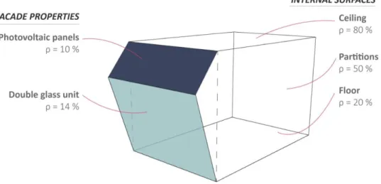
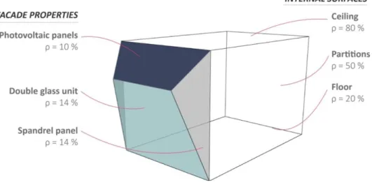
3.6 Elements Properties
The decision of the properties to be assigned the construction elements was influenced by the state of the art reported by the literature. It is a common practice the assignment of the following reflectance values to the different construction elements of the considered zone:
WALL REFLECTANCE: 50% CEILING REFLECTANCE: 80%
FLOOR REFLECTANCE: 20%
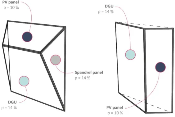
There are referred to the internal surfaces of the zone, while those values which characterize the façade have not been described yet. By means of the following schemes, reporting two of the possible CASE STUDIES we have previously met, all the possible façade materials are introduced. Those cases are considered as samples, are the CASE 2 and CASE 4; in such a way I am considering one of the CASE STUDIES with horizontal layout, and one with a vertical layout. Moreover, in here you may find all the possible materials I will consider in the later simulations: they are only 3 different materials, a glazing unit, a PV panel and a spandrel unit. It is relevant to state again, that the values you are going to read are concerning the only daylight simulations; in fact, there will not be reported any transmittance or thickness values. They will be treated into details later during this research work, as soon as the energy modeling will be implemented during the simulations. The module within the pictures are represented through their metal frames only.
43
3.6.1 Analyses grid
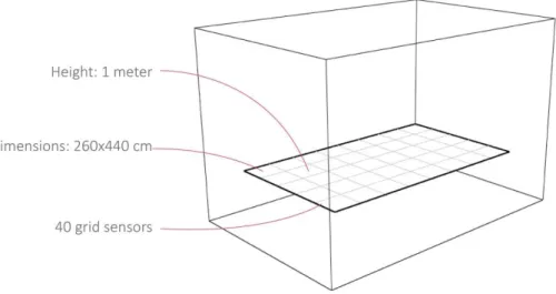
The last required aspect for a daylight simulation is the “grid” which the analyses will based on. The grid is usually placed at a certain height above the floor, which simulates the working plane height within any possible thermal zone; for this reason, a typical value may varies between 70-100 cm. For all the research simulations this height has been chosen equal to 100 cm; moreover, one more operation needs to be done, and that is about the “margin option”. Margin is that space around the zone boundaries, where illuminance data is not to be calculated or included in summary results. As the Designbuilder mentions within its guide, “this option can be used to help avoid inclusion of potentially misleading illuminance data close to walls and windows. A typical margin recommended by CIBSE is 0.5m” 1. By applying this knowledge onto the thermal zone I have previously defined, the grid surface, or better-called testing surface, would result in the following scheme.
Figure 3.2 - Analyses grid description
3.7 Project location
The location chosen is Milan, in Italy, since the research team is based in the same city; this choice could be an advantage, since the standards are known and easily findable and accessible. The location may change in any time of the workflow, but within this thesis it will be kept as it is until the very end of the research. Here follows a picture of the thermal zone in the frame of the sun-path, during the key-days of the year, which are the Solstices and Equinoxes. In such a way, it is possible to have an idea of the sun position in Milan, and which are the criticalities to be faced during the design of a building in this location. The pictures are taken from the DIVA for Grasshopper tool.
44 EQUINOXES 20th March and 22nd September, 12.00 Sun Altitude: 44°
SOMMER SOLSTICE 21st June, 12.00 Sun Altitude: 67°
45 WINTER SOLSTICE 21st December, 12.00 Sun Altitude: 21°
3.7.1 Surrounding Context
All the further analysis have been performed by taking into account the contiguous modules of the façade, by creating a 3x3-modules grid, as it is reported in the following image. In such a way to operate, it is possible to take into account the contribute of the adjacent modules on the considered one, under several points of view.
- Shading effect on the considered thermal one: the thermal zone is affected by the presence of contiguous modules, which are playing the role of shading on it.
- Increase in the PV panel production: as we can observe by looking at the façade with the 9 modules, the geometry and the materials applied on them may increase amount of solar radiation incident on the PV panel (of the considered thermal zone), due to reflection on the glazing modules
- Thermal insulation of the zone: the adjacent modules affects the energy balance of the thermal zone, since they are set with the same internal temperature as the considered zone. In such a way, the losses by conduction and convection towards the external environment will be reduced (same thing for the gains from the outdoor, during summer). Of course, during the analysis of different configurations, the adjacent modules will have the same geometry of the one currently analyzed.
46
Figure 3.3 - Adjacent facade modules
It is important to remind again, that within the first part of the thesis work the context, if meant as surrounding buildings, will not be considered. In fact, the aim is the definition of a fluent workflow for a façade geometry module assessment, and it does not matter if it is approximated or rough, since the most important aspect is the procedure; the context will be implemented in a second stage, when the algorithm will be applied to a real cases study for an hypothetical re-cladding operation. What the reader should always keep in mind, is the possibility of applying the algorithm to any kind of building: for instance, few possible scenarios are represented below, and they are just examples to give the reader an idea of the large-scale of application for the thesis algorithm.
47
3.8 Orientation
Surely, the façade algorithm may be applied to any kind of window exposure, due to the parametric nature of the same algorithm. Anyway, the first part of the thesis, the one where I have to get in touch and familiar with the big amount of data to be managed, the only exposures under analyses will be the Southern and Western one (Eastern as well, since it has same behavior of the Western one). In fact they are the most interesting ones in a location as Milan, as the previous pictures at the chapter §3.7 ”Project location” has shown. It will be certainly an objective of the next simulations the comprehension of how the window exposure affects the façade geometry.
3.9 Analysis period
The analysis period is set to be equal to 1 year, starting on the 1st January and finishing on the 31st December, since the aim is to understand the daylight behavior and guarantee the visual comfort during the whole year. On the other hand, the “analysis period” is a settings like all the other ones, which may be changed whenever the designer desires.
3.10 Schedules
Basically, these schedules concerns the occupancy for the daylight simulations only; in fact, occupancy is represented by means of a “1” value (meaning present) and a “0” value (absent). In the next lines are described 2 schedules, representing the two destination of use previously described. One schedule is simulating an office building and another one for a residential building. It is also important to add that both are set with the DST (Daylight Saving Time); so, schedules are working parallel with the current time changes which happen during the year. Let us see them now, in a graphic way:
- Office Building:
Schedule’s name: Weekdays 8.00-18.00_WithLunchBreak Working days: Mon-Tue-Wed-Thu-Fri
Shutdown days: Sat-Sun Daily Schedule:
Table 3.3 - Office schedule
Hour 0 1 2 3 4 5 6 7 8 9 10 11 On/Off 0 0 0 0 0 0 0 0 0 1 1 1
Hour 12 13 14 15 16 17 18 19 20 21 22 23 On/Off 1 0 1 1 1 1 0 0 0 0 0 0
48
As far as this scheduled is concerned, it is based on the occupancy of a typical office: the workers occupy the building actually only during the working days, from Monday to Friday, each day from the morning at 8.00 till the late afternoon 18.00; the lunch break is set to be from 13.00 to 14.00 on the working days, and the occupancy is set to zero during these breaks.
- Residential Building:
Schedule’s name: AllDays_8.00-19.00
Working days: Mon-Tue-Wed-Thu-Fri-Sat-Sun Shutdown days: None
Daily Schedule:
Table 3.4 - Residential schedule
Hour 0 1 2 3 4 5 6 7 8 9 10 11 On/Off 0 0 0 0 0 0 0 0 1 1 1 1
Hour 12 13 14 15 16 17 18 19 20 21 22 23 On/Off 1 1 1 1 1 1 1 0 0 0 0 0
Another schedule will be considered, the one which permits to simulate the thermal zone as an apartment: in fact, more and more high-rise-residential buildings are under design and development in the world, and for this reason could be interested to simulate the destination of use of the building to residential. It is important to specify the assumption which was assumed during the design of this occupancy schedule: since the sDA and ASE are two metrics which works with percentage of floor area receiving a certain threshold of lux for a certain period of time based on occupied hours, it was reasonable to simulate the occupancy during the only day-time, neglecting the night-time. In this way, the designers may understand the criticalities of a certain curtain walling geometry, basing their simulations on the hours of the day with the sun.
49
Finally, the total occupied hours have been calculated for the two schedules, and their values are reported below. The difference between them is pretty high, it goes up to the 48%, and it would probably affect in a relevant way the daylighting results, since sDA and ASE are metrics based on the occupancy.
50
4
CASE STUDIES
51
4 CASE STUDIES
The natural proceeding of the work, after I have explained also the analyses characteristics, materials properties and boundary conditions, is the simulations phase. Within this chapter the reader may check the results for each one of the 4 CASE STUDIES shown before, and at the end of it there will be a chapter which is totally devoted to the comparisons between them. This chapter represents a phase of the work, that has not been made automatic yet, since a large knowledge of the software is required. So, these simulations helped me a lot understanding the way the software DIVA-for-Grasshopper works, exploring all its functions and options, and discovering eventual problems within the modeling phase. The whole amount of simulations you are going to meet in the next pages, have been performed with DIVA software, in order to evaluate the daylight performance of the thermal zone, by assessing the sDA and ASE values.
4.1 South-facing modules
The attention was addressed at a first stage to the Southern exposure of the curtain walling. In here I have simulated the CASE 1,2 and 3. All of them have been developed into their sub-cases, which means a movement of the control points in a certain direction, in order to slightly change the shape of the façade module, by keeping anyway the same general current CASE STUDY geometry. Moreover, these simulations have been performed with two different possible schedules; these are the one simulating the office space, and the other one the residential building; please visit the chapter§3.10 if you want to check the schedules values. By simulating two schedules, the aim is to show the parametric nature of the façade system, which will certainly adapt their geometry to a certain need, according to the current schedule. The reader will see these geometrical differences, by means of few examples.
Moreover, the results will be shown within each specific paragraph, but the final comparisons among the whole analyzed CASE STUDIES and sub-cases will be treated into details within the chapter§4.3, after the South and West exposure will be widely exhausted.
52
53
4.1.1 CASE 1
As shown in the previous page, where a schematic representation of the CASE 1 was reported, it is clear as the control points will be shifted along both the vertical axes and the direction perpendicular to the façade. The only forbidden movements for the control points, is to move towards each other, otherwise it would change the main geometrical aspect, turning from CASE 1 to CASE 2. By means of the following picture, all the materials used for the daylight simulations are listed: the reader will note that only the reflectances are described, since they are the only property which is required for this kind of simulations. CASE 1 has got only two of the possible façade elements, the glass and the PV panel. On the other side, the parameters of the internal zone are always the same ones.
Figure 4.1 - Elements properties
Different configurations (better called “sub-cases”) have been studied, by varying either the angle or the length of the opaque surface, as follows in the next pictures. The following vertical section shows the two parameters subject to variation: they are the angle “α”, generated between the façade line and the opaque module, and the length “L” of the PV panel on the upper part of the curtain walling module.
54
The way the sub-cases are defined and named is the following one: once the length was kept constant while the angle was subject of variation, and then vice-versa. Those having a constant length are named with numbers from 1 to 7; on the other hand, those having a constant angle but different PV panel length, are called with letters A-F.
Figure 4.3 - Constant PV length sub-cases
Once the 7 cases with different angles were defined, an angle to be kept as fixed was needed to develop the next sub-cases A-F. The Milan location has influenced this choice, and an angle equal to 35° was chosen; actually, this angle guarantees the higher electricity production through PV panels during the whole year. This choice was reasonable in order to keep on pushing the sustainability effort, and try to lower down the electricity demand by means of the PV panels production during the whole year. Remind also that, as previously said, the designer may prefer to simulate solar collectors instead of the chosen PV panels: the parametric characteristics of this workflow I am going to define, makes it possible of course; probably, the most suitable angle in case the solar collectors would replace the PV panels won’t be 35°. In fact, their aim would be the Domestic Hot Water production (DHW), which is an issue to be met mainly during winter; in this way, the solar collector would require an even lower angle “α” since the sun position in winter is much lower than in summer time.
55
On the other hand, the next picture represents the other 6 sub-cases subject to the simulations, as well; they have in common the 35°-tilt-angle, but different PV panels length. Some of them are quite hard to be realized, due to their unconventional dimensions; nevertheless, they are still considered for the simulations, in order to understand their impact on the internal environment. Moreover, it has been widely explained as this phase is focused on the understanding of the façade module behavior, so all the possible scenario are simulated, even if difficult to realize. It will be a further effort, to cut off from the algorithm those complex geometries, by imposing some limits and constraints.
56
4.1.1.1 Results
The whole range based on the 13 sub-cases have been simulated twice, once with the residential schedule, and once with the office space one. The aim is the comprehension of the importance that a schedule plays in the daylighting metrics results. As described at the chapter§3.2.2, metrics such as the sDA and ASE are strictly dependent from the schedule adopted, since they are representing a floor area percentage hit by a certain amount of lux for a certain amount of occupied hours. By reading the next lines, the reader has the chance to note the difference between them, by means of intuitive graphs.
4.1.1.1.1 Residential Use
The graph reported below is the typical one, that has been built up in a customized way, for an easy and intuitive reading of the huge amount of results values. The graph links together the three parameters I have chosen at the beginning of this workflow, and in particular it expresses for each sub-case its comfort condition. The points should be as closest as possible to the grey area, the so-called comfort zone, and ideally they should have been represented witht the biggest circles: this would mean that the current sub-case is guaranteeing the visual comfort and is capturing the highest possible amount of solar radiation. Of course this ideal condition is quite hard to be realized and met, and so let us see their real results within the Graph4.1.
Graph 4.1 - sDA-ASE-IR results
The graph above show the trend of the 13 configurations, according to the 3 parameters I have previuosly described; so, on the x-axis the sDA values are reported, while on the y-axis the ASE
57
values. Furthermore, each point, representing one of the 13 cases, has been represented by means of a cricle, having variable dimension according to the useful incident radiation on the PV panel. The grey area of the graph represents the area where the following conditions are guaranteed, according to the state of art and the rule I have set and described within the previous chapter:
- sDA > 50% - ASE < 10%
We can observe as no cases are placed within this desired zone, but some of them are “floating” close to that zone; for instance cases 5 and C have a high value of sDA but they are not fitting the ASE limit, even if they could have acceptable values of it, especially case 5 which has also a pretty high amount of incident solar radiation. On the other hand, cases 2,3 and D do not respect the sDA limit, but they have a value of ASE close to the 10% boundary, and a solar radiation higher than 6000 kWh. Surely, case 4 is the one which is the closest to the grey area, even if its sDA is not so high and satisfying.
At a first glance at the same Graph4.1, it is clear the overall distribution of the results; it is in fact a curve which tends to the 0% of both sDA and ASE. By means of the following Graph4.2, the reader may also have a comprehension of the general trend of the results.
Graph 4.2 - Results trend
The common rules are the following ones:
- Constant angle sub-cases: the longer is the PV panel with the constant 35°-tilt-angle, the darker is the internal room;