Simultaneous Localization and Mapping Technologies

(1)

ALMA MATER STUDIORUM - UNIVERSIT `

A DI BOLOGNA

CAMPUS DI CESENA

Scuola di Ingegneria e Architettura

CORSO DI LAUREA MAGISTRALE IN

Ingegneria Elettronica e Telecomunicazioni per l’Energia

SIMULTANEOUS LOCALIZATION AND

MAPPING TECHNOLOGIES

Elaborato in

Reti di Sensori Wireless per Monitoraggio Ambientale

Relatore

Chiar.mo Prof. Ing.

DAVIDE DARDARI

Correlatore

Dott. Ing.

NICOL `

O DECARLI

FRANCESCO GUIDI

Presentata da

NOUR NAGHI

Sessione III

Anno Accademico 2017-2018

(2)

(3)

Abstract

Il problema dello SLAM (Simultaneous Localization And Mapping) consiste nel mappare un ambiente sconosciuto per mezzo di un dispositivo che si muove al suo interno, mentre si effettua la localizzazione di quest’ultimo.

All’interno di questa tesi viene analizzato il problema dello SLAM e le dif-ferenze che lo contraddistinguono dai problemi di mapping e di localizzazione trattati separatamente.

In seguito, si effettua una analisi dei principali algoritmi impiegati al giorno d’oggi per la sua risoluzione, ovvero i filtri estesi di Kalman e i particle filter.

Si analizzano poi le diverse tecnologie implementative esistenti, tra le quali figurano sistemi SONAR, sistemi LASER, sistemi di visione e sistemi RADAR; questi ultimi, allo stato dell’arte, impiegano onde millimetriche (mmW) e a banda larga (UWB), ma anche tecnologie radio gi`a affermate fra le quali il Wi-Fi.

Infine, vengono effettuate delle simulazioni di tecnologie basate su sistema di visione e su sistema LASER, con l’ausilio di due pacchetti open source di

MATLAB. Successivamente, il pacchetto progettato per sistemi LASER `e

stato modificato al fine di simulare una tecnologia SLAM basata su segnali Wi-Fi.

L’utilizzo di tecnologie a basso costo e ampiamente diffuse come il Wi-Fi apre alla possibilità, in un prossimo futuro, di effettuare localizzazione indoor a basso costo, sfruttando l’infrastruttura esistente, mediante un sem-plice smartphone. Più in prospettiva, l’avvento della tecnologia ad onde millimetriche (5G) consentirà di raggiungere prestazioni maggiori.

(8)

(9)

Keywords

SLAM Mapping Localization Indoor EKF RADAR LASER LIDAR UWB mmW Visual

(10)

(11)

List of Abbreviations

SLAM Simultaneous Localization And Mapping PF Particle Filter

RBPF Rao-Blackwellized Particle Filter KF Kalman Filter

EKF Extended Kalman Filter PDF Probability Density Function FB Feature Based

OGB Occupancy Grid Based MD Mobile Device

RD Reference Device

RSS Reference Signal Strength TOA Time Of Arrival

TDOA Time Difference Of Arrival PDOA Phase Difference Of Arrival AOA Angle Of Arrival

LOS Line Of Sight

IMU Inertial Measurement Unit INS Inertial Navigation System CPU Central Processing Unit

(12)

CPU Graphics Processing Unit MSE Mean Squared Error

MMSE Minimum Mean Square Error MAP Maximum A-Posteriori

ML Maximum Likelihood

BLUE Best Linear Unbiased Estimator EKF Extended Kalman Filter

GPS Global Positioning System

LASER Light Amplification by Stimulated Emission of Radiation RADAR Radio Detection And Ranging

LIDAR Laser Imaging Detection And Ranging SONAR Sound Navigation And Ranging UWB Ultra Wide Band

mmW millimetre Wave 2D 2 Dimensional 3D 3 Dimensional

(13)

Chapter 1 Introduction

The Simultaneous Localization And Mapping (SLAM) problem consists in the simultaneous reconstruction of an unknown environment and the local-ization of a device moving within it. This problem is more general and harder than the single mapping or localization problems, that can be seen as particular cases of SLAM.

In the mapping problem, the device is aware of his absolute location, so it can use this information along with the data coming from the sensors observing or interacting with the environment to infer its topological map.

In the localization problem, a map or some reference devices are made available in order to obtain the position of the device observing or interacting with them.

The scenarios where there is not any a-priori knowledge related to location and map, are those in which the SLAM becomes necessary.

Many applications require the reconstruction of a consistent map; in geral, in many applications, a robot may have the goal of exploring an en-vironment and report it to a human operator. For instance, if we consider outdoor autonomous navigation of robots, if the robot has access to GPS, the SLAM is not required; conversely, in indoor environments, the use of GPS for localization scope is ruled out.

The solutions to this problem are employed in several applications includ-ing:

Self-driving cars and drive assistance systems Unmanned Aerial Vehicles (drones)

Autonomous Underwater Vehicles Planetary rovers

(14)

Domestic robots Security systems

Autonomous navigation of robots Augmented reality

This thesis aims at understanding the general SLAM problem and his main techniques of resolution, investigating the actual state of the art and simulating through MATLAB different technologies.

It is suddivided in the following chapters:

Mathematical tools for the study of dynamic physical systems: the mathematical tools useful for the comprehension and the study of the SLAM topics are here introduced and explained; specifically, the math-ematical representation of a physical dynamic system and the methods for the implementation of Bayesian filters are put in evidence.

Localization and mapping in dynamic physical systems: this chapter focuses on the general definition of localization, mapping and SLAM problems and the differences between them.

State of the art related to the SLAM problem: here a general view on the state of the art is given; the anatomy of a SLAM implementation is viewed and the main technologies exploited are treated.

MATLAB implementation of different SLAM technologies: The exper-imental simulations done on different technologies are here analyzed; Two different SLAM toolbox implemented in MATLAB are exploited; the first is based on vision and the second on the LASER.

(15)

Chapter 2 Mathematical tools for the

study of dynamic physical

systems

In this chapter, the mathematical tools useful for the comprehension and the study of the topics that are covered in this thesis are put on focus.

In particular, the mathematical tools that are used nowadays to solve the SLAM problem are going to be analyzed: in the next subchapters, the following topics are taken into consideration:

The numerical representation of a physical dynamic system The Bayesian filter, used to estimate the state of a system

A few existing techniques for the implementation of a Bayesian filter, including the Kalman filter, the extended Kalman filter and the particle filter

2.1 Representation of a physical dynamic

sys-tem

In the study of a physical dynamic system, the estimation of the state is needed, starting from the noisy measurements performed on the system, in order to let the controller act consequently through a control signal on the actuator; this process is described in figure 2.1. The state of the system evolves in time and is conditioned by uncertainty, just like the measurements performed on it; generally, the estimation process of the state may generate optimal solutions with MMSE techniques (Minimum Mean Square Error),

(16)

Figure 2.1: Representation of the control on a dynamic physical system[1]

but at the cost of large computational expenses, so that recursive approaches are preferred, since they are characterized by a lower complexity and the possibility to perform the estimation in real-time.

Physical systems are modelled by differential equations and a state space; since computers only process discrete-time data, this model is taken over by his numerical translation based on difference equations and discrete state space, where the involved variables are described as follows

xn = f (xn−1, un) (2.1)

y_n= h(xn, un) (2.2)

where:

xn represents the state vector at the instant n

yn represents the measurements vector at the instant n

un represents the action of the controller at the instant n

What has been described is valid only for deterministic systems, but if uncertainties are characterized by random processes, it becomes necessary to switch from the study of deterministic functions to the study of conditioned transition probability density functions (PDF) that are described as follows p(xn|x0:n−1, u1:n) (2.3)

p(y_n|x0:n−1, y1:n−1, u1:n−1) (2.4)

where:

(17)

u1:n represents the whole set of control actions until the instant n

y1:n−1 represents the whole set of measurements until the instant n − 1

An instance of a linear model with Additive Gaussian Noise is the follow-ing

xn= Axn−1+ Bun+ wn (2.5)

The purpose is to obtain the best estimate (e.g., in the MMSE sense) of the succession of states of the system until an instant n (namely statistical inversion or optimal filtering):

x0:n= {x0, x1, ..., xn} (2.6)

starting from a succession of n measurements until the instant n

y_0:n= {y₀, y₁, ..., y_n} (2.7)

Solving this problem means calculating the a-posteriori joint probability distribution of the whole sequence of states n given all the noisy measure-ments and the control actions until the instant n:

p(x0:n|y1:n, u1:n) =

p(y_1:n, u1:n|x0:n)p(x0:n)

p(y_1:n, u1:n)

(2.8) where:

p(x0:n) is the a-priori PDF of the succession of states

p(y1:n|u1:n, x0:n) is the likelihood function of the noisy measurements

and the control actions

p(y1:n, u1:n) is a normalization constant

Regarding the problem treated in this thesis, starting from the noisy observa-tions y_0:n and the control actions u1:n, what is wanted is not the resolution of

the whole succession of states x0:n, which can be done only after all

measure-ments have been collected, then not in real time; it is wanted the resolution of the single current state xnfor each instant n, using the marginal a-posteriori

PDF, called belief

Bel(xn) = p(xn|y1:n, u1:n) (2.9)

(18)

2.2 Bayesian filters

The main drawback in applying the 2.9 is that it has to be recomputed whenever a new measurement is taken, making the computational complexity intractable as n increases. Thanks to the Bayesian filters, the complexity can be drastically reduced exploiting the following Markov hypothesis [8]:

The state at the step n depends only on the immediately preceding state xn−1 and the applied control un, while it is independent of the

observations

p(xn|x0:n−1, y1:n−1, u1:n−1) = p(xn|xn−1, un) (2.10)

This PDF is called motion or mobility model [5]

The current noisy observation yn is independent of the previous states,

input controls and observations, but depends only on the current state xn

p(y_n|x0:n−1, y1:n−1, u1:n−1) = p(yn|xn) (2.11)

This PDF is called perception, measurement or observation model [5] These hypothesis allow to get the Markovian model of the state space, which is characterized from the following properties:

At first, the a-priori PDF p(x0) is used to define the initial uncertainty

of the system state

The observation model of the system p(yn|xn), shows the dependence

of the noisy measurements at a certain instant from the state at the same instant

The system state dynamics is described by the mobility model p(xn|xn−1, un)

(19)

The Bayesian filter is a recursive estimator that at every step exploits the mobility model p(xn|xn−1, un), the control action un and the new

measure-ment y_n to get the belief of the current state starting from the one of the previous instant p(xn−1|y1:n−1) (figure 2.2)

The estimation of the state occurs according to the following iterative procedure, also illustrated in figure 2.3:

The a-priori PDF of the state p(x0) poses as the initial belief of the

state;

Figure 2.3: Flux diagram of a Bayesian filter [1]

The prediction step (figure 2.4) is performed (obtained exploiting the 2.10) [8]

p(xn|y1:n−1, u1:n) =

Z

p(xn|xn−1, un)p(xn−1|y1:n−1, u1:n−1) dxn−1

(2.12)

The update step (Figure 2.5) is realized (obtained exploiting the 2.11) [8] [1]

p(xn|y1:n, u1:n) =

p(y_n|xn)p(xn|y1:n−1, u1:n)

R p(y_n|xn)p(xn|y1:n−1, u1:n) dxn

(2.13) Once obtained the belief of the state n, it is possible to use it to estimate

(20)

Figure 2.4: Prediction step [1]

(21)

– MMSE: ˆ xM M SE_n = Z xnp(xn|y1:n, u1:n)dxn (2.14) – MAP ˆ xM AP_n = argmaxxnp(xn|y1:n, u1:n) (2.15) –

It is well known that when the posterior distributions are Gaussian, the MAP and MMSE estimates coincide [8]. This method makes it unnec-essary to recalculate equation 2.8 at each time instant; this procedure would involve the whole sequence of states and measurements in the computation. Instead, the Bayesian filters use at every step the current data to recursively update the belief.

2.3 Kalman filters

The Kalman filter (KF) is a closed form solution that is used to implement a Bayesian filter; it applies when the observation and mobility models are linear and the noise is Gaussian according to the following equations:

xn = An−1xn−1+ Bnun+ wn (2.16)

y_n= Hnxn+ νn (2.17)

with

wn= N (0, Qn) process noise

νn = N (0, Rn) measurement noise

Hence the following mobility model and marginal a-posteriori PDF is obtained

p(xn|xn−1) = N (xn; An−1xn−1+ Bnun, Qn−1) (2.18)

p(y_n|xn) = N (yn; Hnxn, Rn) (2.19)

(22)

Made these premises, the Kalman filter is an algorithm that calculates in a recursive way the parameters m−_n, mn, P−n, Pn. Practically, the calculation

of the PDF is not made in every point, but only the mean values and the covariance matrices are calculated, from which it is possible to exhaustively describe a Gaussian PDF.

The Kalman Filter is realized by the following update equations related to the steps previously introduced (2.12,2.13):

Prediction step: m−_n = An−1mn−1+ Bnun (2.22) P−_n = An−1Pn−1ATn−1+ Qn−1 (2.23) Update step: vn= yn− Hnm−n (2.24) Sn = HnP−nH T n + Rn (2.25) Kn = P−nH T nS −1 n (2.26) mn= m−n + Knvn (2.27) Pn = P−n − KnSnKTn (2.28) where:

vn is called innovation, that is the difference between the expected

measurement at the instant n, based on the belief N (m−_n, P−_n) obtained in the previous step, and the actual measurement yn.

Kn is the Kalman gain, that is a parameter that lets the algorithm

update the state in function of the current measurement according to the reliability of the current measurement.

The Kalman filter is the optimum filter when the model is linear with additive Gaussian Noise; conversely, when the noise is not Gaussian, the Kalman filter is not in general optimum, but it represents the Best Linear Unbiased Estimator (BLUE). When the model is not linear or Gaussian it is in general

no more optimum. mn can be used as the point estimate at time step n,

(23)

2.4 Extended Kalman filters

It often happens in practical applications that the dynamic and measurement models are not linear and the Kalman filter is not appropriate. However, of-ten the filtering distributions of this kind of model can be approximated by Gaussian distributions. The Extended Kalman Filter (EKF) is then appli-cable through the linearization of the non-linear models showed in 2.29 and 2.30 by using Taylor series [7]:

xn= f(xn−1, un) + qn−1 (2.29)

y_n = h(xn) + rn (2.30)

where

f represents the dynamic model function h represents the measurement model.

The stochastic translation of these models assumes Gaussian distribution for the mobility model and the perception model, in order for the EKF to be applicable as follows:

p(xn|xn−1) = N (xn|f(xn−1, un), Qn−1) (2.31)

p(y_n|xn) = N (yn|h(xn), Rn) (2.32)

The linearization through Taylor series allows to approximate also the PDF of the belief into a Gaussian distribution as follows:

p(xn|y1:n) ' N (xn|mn, Qn) (2.33)

The algorithm that realize this approximation is described by the follow-ing prediction and update steps:

Prediction step m−_n = f (mn−1, un) (2.34) P−_n = Fx(mn−1)Pn−1FTx(mn−1) + Qn−1 (2.35) Update step vn= yn− h(m − n) (2.36) Sn = Hx(m−n)P − nH T x(m − n) + Rn (2.37) Kn = P−nH T x(m − n)S −1 n (2.38) mn = m−n + Knvn (2.39) Pn= P−n − KnSnKTn (2.40)

(24)

where

Fx is the Jacobian matrix of f

Hx is the Jacobian matrix of h

It has to be taken into consideration that the algorithm here discussed realizes the first order additive noise EKF and it will not work when con-siderable non-linearities are present. The filtering model is also restricted in the sense that only Gaussian noise processes are allowed.

The EKF also requires the measurements model and the mobility model functions to be differentiable. Moreover, the Jacobian matrices.

On the other hand, with respect to other non-linear filtering methods, the EKF is relatively simple compared to his performance and is able to represent many real cases [7].

2.5 Particle filters

When a linear model of the system and a Gaussian noise model are not suitable for the system, the utilization of an EKF becomes pointless. The same statement can be made when the PDF are multimodal or discrete. In this case the implementation of a Particle Filter (PF), also known as Sequential Montecarlo Method becomes useful.

Here the belief is represented as a set of Dirac deltas (particles): Bel(xn) = X i wiδ(xn− xin) (2.41) where wi

n are the importance factors: they are weigths that describe the

prob-ability to be in a certain state xn at every step n.

The set of weights wi

n is updated at every step according to the new

control un and the new measurement yn, starting from the old one win−1.

The particle filter may suffer from the weights degeneration problem as at every step all weights are multiplied by a factor less than 1, thus lead-ing to a set of weights where all but a few particles have negligible weights. This problem is unavoidable and is shown in 2.6: in this instance, an initial a-priori PDF p(xn−1) sampled into weights, is conditioned by a new

mea-surement yn and leads to the resulting belief, which weights are now weaker

then the former. A procedure of resampling must be actuated whenever the degradation is detected as shown in 2.7; the resampling must be performed with a major density where the weights are greater [4].

(25)

(26)

(27)

Chapter 3 Localization and mapping in

dynamic physical systems

The SLAM problem (Simultaneous Localization And Mapping) is known as the issue of building, or updating, the map of an unknown environment, using the observations collected by a device that explores it, while tracking itself. Compared to the classic mapping problem in which the location of the object is known during the mapping, here the localization task has to be performed in the absence of reference nodes (often called ”anchor nodes”), i.e., in the absence of a dedicated infrastructure. Generally for the resolution of this problem successive approximation methods like the Particle Filter(PF) and the Extended Kalman Filter(EKF) are adopted. The SLAM algorithms are tailored in function of the available informations and resources.

Before dealing with the SLAM problem, a general view on the separated problems regarding the mapping and the localization is here given.

3.1 The mapping problem

The mapping problem is considered as a simplified SLAM problem, in which the mobile location is assumed known (in figure 3.1, a vehicle maps the surrounding environment using the GPS to obtain his position)

The issue can be formalized as follows: the a-posteriori PDF P (mn|y1:n),

conditioned on the observations y_1:n, has to be estimated given the series of (known) positions of the device x1:n, in order to estimate the state vector of

the system, using a chosen criterion. mn is the state vector and it usually

contains the positions of the landmarks representing the environment in an instant n mn= [m(1)xn, m (1) yn, m (2) xn, m (2) yn, ..., m (N ) xn , m (N ) yn ]

(28)

where N is the number of landmarks. The mapping problem can be treated with different approaches regarding the representation of the environment, that can be resumed in three categories:

Figure 3.1: A mobile vehicle that performs mapping using a LIDAR system (https://hu.wikipedia.org/wiki/F´ajl:LIDAR equipped mobile robot.jpg)

Feature Based approach (FB): here the environment can be modeled as a collection of entities called features, that code all the relevant infor-mations concerning walls, edges, corners, objects and other obstacles. The mapping problem is all about estimating the state of each feature, whose main element is the position, although it may include orienta-tion, colour or other properties [2].

(29)

From the computational point of view, this is a fast approach that does not require a considerable occupation of memory, but since the extracted features are predefined, an a-priori knowledge of the environ-ment structure becomes necessary. Generally, this approach is preferred when the mapping must be performed in outdoor contexts, where there are large spaces and few landmarks [3].

Occupancy Grid Based approach (OGB): the space here is decomposed in a grid of cells, each one characterized by an occupation PDF; the latter must be used to estimate whether or not an obstacle is present. The computational burden and the necessary memory to save all the informations is greater than the FB. Moreover, to correct the mobile position, the detection of a certain number of obstacles becomes nec-essary, hence in presence of large spaces with very few landmarks and limited spatial scan available, this approach can enter into crisis. On the other hand, the capability to represent objects and obstacles of any shape is achieved. Generally, this approach is preferred in indoor environment [3].

Mixed approach: the purpose of this approach is to improve the per-formances when the mapping of environments with a few features and indoor contexts are both needed; at every step, based on the current measures, the state is updated and one of the previous approaches can be implemented. In this way, the representation of a mixed environ-ment is possible without suffering too much from the drawbacks of each technique. [3].

3.2 The localization problem

The localization problem consists in identifying the position of a device that is situated inside a map that is assumed known (figure 3.2). This issue can be formalized as follows: the a-posteriori PDF P (xn|y1:n), conditioned from

the observations y_1:n, has to be estimated given the series of landmarks of the environment m1:n assumed known and typically named anchors or reference

devices (RDs), in order to estimate the position of the device, using a chosen criterion.

xn is the state vector, that mainly contains the positions of the device

and, possibly, its speed and orientation at the instant n xn= [xxn, xyn, vxn, vyn, oxn, oyn]

(30)

Figure 3.2: Representation of the localization problem

The localization problem can be treated with different approaches; the main methods are the following:

Triangulation: this type of method exploits the geometric relationship between the mobile device (MD) and the reference devices (RDs). For this purpose, different properties of signals exchanged among them can be used [4]:

– Received Signal Strength (RSS) – Time Of Arrival (TOA)

– Time Difference Of Arrival (TDOA) – Phase Difference Of Arrival (PDOA) – Angle Of Arrival (AOA)

Fingerprinting: this method involves measuring position-dependent fin-gerprints of the signal at known positions to construct a fingerprint database of an environment that can be used to localize and track the MD. Generally, it is composed of two steps: the first one is to collect the position-dependent fingerprints into a database, while the second deals with matching the measured fingerprints of the MD with those of the database through a pattern-recognition algorithm, in order to lo-cate and track the MD. It can be adopted when the line of sight (LOS) path is blocked, which typically makes it difficult to apply geometric relationships between MD and RDs.

(31)

Proximity: proximity-based techniques rely on a dense grid of RDs pre-viously deployed at known positions in an environment. Each RD has got its own detection radius. Once the MD enters an RD’s detection region, the MD and this RD are connected; according to this connec-tion, the MD is localized. This kind of technique requires a simple receiver architecture, but also a pre-deployment of dense grids of RDs. In advance, when multiple RDs detect the MD, more sophisticated smoothing method are needed, even though the localization accuracy could be poor compared to other methods.

Self-measurements: Unlike the types of measurements mentioned above that rely on an infrastructure, self-measurements can be collected by a stand-alone MD with an Inertial Measurement Unit (IMU). Typically, an IMU is composed of a 3D gyroscope and a 3D accelerometer, which provide angular velocity and linear acceleration, respectively. Given the initial position and the MD’s velocity and orientation information, the standalone MD can be localized and tracked by integrating the measured angular velocity and linear acceleration with the Bayesian filters. However, the measurement errors of the IMU will be integrated and propagated unbounded over time, which limits stand-alone inertial localization and tracking with a low-cost IMU [4].

3.3 The SLAM problem

The SLAM problem merges the previous presented issues of building the map of an unknown environment and localizing the mobile device within it. Both the trajectory of the MD and the location of all landmarks are estimated online without the need for any a-priori knowledge of location (figure 3.3).

The formalization of this problem follows: considering a mobile robot moving through an environment and taking relative observations of a number of unknown landmarks, at a time instant k, the following quantities are defined:

xn: the vector that describes the location and orientation of the vehicle

at time n

xn= [xxn, xyn, vxn, vyn, oxn, oyn]

un: the control vector, applied at time n-1 to drive the vehicle to a

(32)

Figure 3.3: Representation of a SLAM problem: both location of the MD and landmarks are estimated[5]

mn: a vector describing the locations of the landmarks whose true

location is assumed time invariant at a time n

mn = [m(1)xn, m(1)yn, mxn(2), m(2)yn, ..., m(N )xn , m(N )yn ]

yn the vector of the observations taken from the vehicle related to the

locations of the landmarks at time n

y_n= [y_xn(1), y_yn(1), y_xn(2), y_yn(2), ..., y(N )_xn , y(N )_yn ] x1:n: the history of vehicle locations

x0:n= x0, x1, ..., xn

u1:n: the history of control inputs

u1:n= u1, u2..., un

y1:n: the history of all the observations performed on the landmarks

(33)

The SLAM problem requires the computation of the a-posteriori PDF

P (xn, mn|y1:n, u1:n, x0) (3.1)

that is conditioned on the observations y_1:n, the control inputs u1:n and the

initial state x0 without any information regarding his location or the

land-marks of the environment. The aim is to estimate, using a chosen criterion, the state vector of the system, which in this case is the union of the vectors xn and mn and contains both the estimated device location and map

in-formation [5]. To this purpose, many statistical algorithms can be employed based on Bayesian Filters, in particular Extended Kalman Filters (EKF) and Particle Filters (PF).

(34)

(35)

Chapter 4 State of the art related to the

SLAM problem

The autonomous navigation in unknown spaces requires the capability of a mobile robot to be aware of his location and the locations of other places of interest nearby. This is one of the main skills that a mobile autonomous robot should achieve. Many devices base this capability in prior reliable mapping or positioning information such as the Global Positioning System (GPS).

In first place, without a notion of location, a robot is limited to reactive behaviour based solely on local stimuli and is incapable of planning actions beyond its immediate sensing range [9]. The quality of localization is clas-sically driven by the reliability of the provided map: in the absence of the latter, dead-reckoning methods would quickly drift over time, while the use of a map of the environment allows the reset of the localization error by revisiting the known areas: this concept is known as loop closure.

The resolution of the SLAM problem enables a robot to navigate any un-known environment without the need for prior map or location information; this allows the approaching to a more independent behaviour of the robot, where all high level navigation operations such as goal reaching, region cov-erage, exploration and obstacle avoidance are carried out without external support.

This brings to the main reason for which the SLAM is needed: the scenar-ios in which a prior map is not available need the simultaneous reconstruction of both environment and location[10].

(36)

4.1 Anatomy of a SLAM system

The architecture of a SLAM system can be divided in a front-end component and a back-end component. The front-end role is to abstract sensor data into estimation models like those described in Chapter 1, while the back-end performs inference on the abstracted data produced by the front-end [10]. This architecture is shown in figure 4.1.

Figure 4.1: Front-end and end in a typical SLAM system. The back-end can provide feedback to the front-back-end for loop closure detection and verification [10]

4.1.1 Back-end

The back-end component of the system must provide an estimation of the state based on the belief defined in Chapter 1 (2.9): as mentioned before, the state typically includes the estimated pose of the robot (location and orientation) and the position of landmarks in the environment; the belief is generally obtained using an improved version of the EKF and PF presented in Chapter 1.

(37)

Figure 4.2: Representation of the SLAM with factor graphs [10]

The EKF is still largely diffused in SLAM applications because of his linear Gaussian assumptions in the representation of both the measurement and motion model.

When linear measurement and motion model are not available and the noise of the system can not be assumed Gaussian, the PF, based on Monte Carlo sampling, must be used. The main drawback is that the application of particle filters on the high dimensional growing state-space of the SLAM problem is unfeasible; however, through Rao-Blackwellization, a joint state can be partitioned according to the product rule, obtaining the so called Rao-Blackwellized Particle Filter (RBPF); as an instance, here is a joint PDF of 2 states:

p(x1, x2) = p(x2|x1)p(x1) (4.1)

In this way, if p(x2|x1) is available,only p(x1) needs to be sampled,

sim-plifying the estimation of the joint state; this technique allows the factor-ization into a vehicle component and a conditional map component of the joint SLAM state, that improves the speed of the algorithm as the map is represented as a set of independent Gaussian processes [5]. The RBPF

Currently, many approaches formulate SLAM as a MAP estimation prob-lem, often using the formalism of factor graphs [10]: the dependence of poses and landmarks, both represented as circles, from each other are put in evi-dence with the aid of factors related to:

(38)

Odometry constraints: if they link two poses

Sensor observations: if they link a pose and a landmark Loop closure: if an event of loop closure is detected

This can be considered a more general approach with respect to Bayesian filtering based on the message passing of beliefs.

In figure 4.2, is shown a simple factor graph representation that highlights the main dependence of different variables at consecutive time steps, where:

(x1; x2; ...) is the sequence of robot poses

(Lmk1; Lmk2; ...) is the sequence of landmarks positions

(u1; u2; ...) is the sequence of motion controls

(v1; v2; ...) is the sequence of measurements

K is the set of intrinsic calibration parameters (c1, c2, ...) is the set of closure loops

The main advantages brought by the factor graph representation of the SLAM problem can be resumed in:

Simplification of the view, that can be appreciated in figure 4.2

Generality of the problem, enabling the modeling of complex problems through interconnections of heterogeneous variables and factors; this approach

4.1.2 Front-end

Generally, is hard to use all the sensor measurements for the MAP estimation because they should all be expressed as analytic function of the state. This justifies the presence of a front-end module that extracts only the relevant features from the sensor data [10].

The front-end also deals with the problem of associating each measure-ment to the correct landmark; this problem is commonly addressed as data association.

(39)

4.1.3 Odometry

According to the odometry principle, if a robot is aware of his position and his future movements than he is aware of his pose. Knowing the motion model of the robot, his initial pose and a global reference coordinate system, localization is doable.

As an instance, wheel odometry uses sensors mounted on wheels to mea-sure the travelled road and estimate the trajectory. The main limit of this method is the accumulated measurement error that becomes dominant over time causing estimated robot pose to drift from its actual location. This effect is showed in figure 4.3. Another source of error that should not be underestimated is wheel slippage in uneven terrain or slippery floors: if the world is modelled as a plane, a non-flat ground surface may cause estimated and real position to take different directions, while slippage can be responsi-ble of mismatches of actual and estimated travelled road.

Figure 4.3: Representation of the accumulated odometry measurement error This problems are significantly reduced through the use of an Inertial Measurement Unit (IMU): it is a device that exploits a triaxial gyroscope and a triaxial accelerometer to track acceleration, deceleration and position

(40)

(through a double integration of the acceleration), of the vehicle in which is mounted. This makes possible the detecting of changes in direction and velocity, allowing an augmented odometry. Conversely, IMU fails in obser-vation of low-frequency faults such as model biases, which might lead to error accumulation. . For this reason, IMU is suited for the detection of low term motion, between the map observations, but is not sufficient for longer term[9]. IMUs are widely used in Inertial Navigation Systems (INS), that are aid systems for aero-mobile navigation mainly made of an IMU, sensors and a CPU, and in advanced automotive and motorcycle industry and in robotics.

Visual Odometry is the current state of the art and uses the images seen from a single or multiple camera to estimate the ego motion of the vehicle in which is mounted. It is demonstrated that this system performs better than wheel odometry or LASER scanners [12].

4.1.4 Sensors in SLAM

In addition to the already mentioned sensors that implement odometry, there are different kind of sensors that are used to perform SLAM. They exploit interactions with landmarks to estimate the state of the system, including pose of the robot and pose of landmarks.

The type of sensor used is what mainly differentiate a SLAM system and his applications from another one. Another way to see the matter is the following: both SLAM sensors and odometry perform sensing activity, each one on a different subject, then they cooperate fusing the obtained data for the achievement of the same goal.

As previously mentioned, a SLAM technology depends on the type of sensor implemented; the main branches of the current state of art are the following and are deepened in the next section:

SONAR SLAM RADAR SLAM LASER SLAM Visual SLAM

4.2 The main SLAM technologies

SLAM requires the simultaneous reconstruction of the environment and the pose of a robot inside it. The context in which SLAM is needed can influence

(41)

the choice of the technology. As an instance, in undersea environment the main reliable technology is SONAR due to the distortion that water imprints to light. A glance of the main technologies developed until now follows.

4.2.1 SONAR SLAM

SONAR means Sound Navigation And Ranging and is a system which ex-ploits an acoustic sensor to perform the propagation of ultrasounds and the following reception of their reflected version whether an obstacle is present.

Figure 4.4: SONAR systems are commonly used by ships to probe the seabed

Mobile robot navigation and mapping is far more difficult using SONAR sensor, instead of a LASER one as an instance. A reason is the modest spatial resolution obtained using the former in comparison to the latter; another one is that SONAR is characterized by an inferior degree of accuracy with respect to LASER; last but not least, is the lower speed of response with respect to the other sensors here presented.

Despite these difficulties, SONAR SLAM is still interesting to research for some reasons. SONAR sensors are less expensive than LASER scanners, as an instance, actually ultrasonic sensors are the cheapest available source of spatial sensing for mobile robots. Furthermore, they suffer of lower signal attenuation in underwater environment, where visual and LASER sensors are ruled out from this point of view due to their high frequency signals

(42)

[13]. Thus, SONAR sensors become the ideal sensor with whom an AUV (Autonomous Underwater Vehicle) can perform SLAM.

SONAR SLAM systems exploit transceivers characterized by low fre-quency sound waves which allow deep penetration of water (10-150 m), while high frequency signals like those of LASER are highly attenuated. Time of flight methods are used to localize the landmarks [14].

4.2.2 RADAR SLAM

The meaning of RADAR is Radio Detection And Ranging and it represents a system that employs radiating electromagnetic waves (EM waves) to let a transceiver detect whether they are reflected from an obstacle. In figure 4.5 is shown the exchange of two RADAR signals for the identification of an airplane. The working principle is the same as SONAR, except for using EM waves instead of acoustic waves.

Figure 4.5: RADAR systems are widely used for aerospace purposes This technology enables SLAM in situations where visibility is compro-mised such that Vision and LASER systems are not suitable; an example is an emergency scenario like a fire, where dust and smoke are present and can impede to individuate not only walls and objects but also unconscious peo-ple. Millimetre Wave RADAR SLAM (mmW RADAR SLAM) technology and UWB RADAR SLAM technology are now the main branch in develop-ment in RADAR area [18].

Many works certify the robustness of this technology; to mention one, in [19] is showed an approach that exploits the specular reflections of EM waves on flat surfaces in order to localize a mobile user using the reflections coming

(43)

from just one reference node. The concept of virtual anchor, which is the mirror image of a physical anchor, is then used in order to use the multipath components to do the SLAM estimate.

Under study is also the possibility to perform SLAM using Wi-Fi signals, considering access point as landmarks, with the purpose of localization inside a building. The main obstacle is that Wi-Fi standard, as well as other pos-sible suited technologies like RFID, NFC and ZigBee to mention some, were not created with localization or mapping purpose [15] [16] and hence they typically provide measurements scarcely related to distance or position. The crowd-sensing concept can however come to help: this principle is due to the consideration that nowadays most people are provided with a smartphone equipped with a large bunch of sensors (light, temperature, pressure, sound, acceleration and magnetism can be sensed) [8].

The idea behind crowd sensing is to mitigate the scarce accuracy of mea-surements through the exploitation of a huge amount of meamea-surements shared among users.

Mentioned this, let us have a look at main RADAR technologies.

Ultra Wide Band SLAM

Ultra Wide Band (UWB) RADAR SLAM Technology has grown since 2002, when Federal Communications Commission opened up 7,5 GHz of spectrum (from 3,1 to 10,6 GHz) to be used by UWB devices.

This system exploits narrow time-domain pulses, of a duration in the order of a nanosecond, to modulate a signal spreading his spectrum over a wide frequency band larger than 500 MHz. The main advantage of this method is the higher resolution in estimation of the time of flight, which translates in ranging estimation with few centimetre accuracy [15].

An interesting example of UWB SLAM system is presented in [17] where the implementation of a small antenna array of bat-type, which is made of two receiving antennas and a transmitting one allows more advantages, like the individuation of different landmark types.

Millimetre Waves SLAM

In the last decade, mmW RADAR SLAM has gained popularity in research because where low frequency radio signals have a wide beam width, which reduces the resolution in detecting the obstacles, mmWs allow narrow beam shaping, thus augmenting the resolution in detecting obstacles with respect to lower frequency radio signals.

(44)

mmWs belong to the band of radio waves with frequency going from 30 to 300 GHZ. This band is commonly known as Extremely High Frequency range and their wavelength ranges from 10 to 1 mm.

In a SLAM application, an array of antennas can be used to achieve a determinate angular resolution through use of mmW; the same can be done with UWB signals, but since the wavelength is lower, the compactness for the achievement of the same result is greater.

mmWs are subject to a high atmospheric attenuation which reduces the range and strength of the waves. Thus, they are limited in a communica-tion range of about 1 kilometre. mmW RADAR SLAM signals are able to penetrate many objects and can provide information regarding distributed targets appearing in a single observation[16].

Figure 4.6: The detection of different types of landmarks is possible using a bat-type array of antennas [17]

4.2.3 LASER SLAM

The LASER working principle is the same of SONAR and RADAR and differently from the latter, here EM waves are in the range of UV, visible or infrared; this allows the reflection of waves from very small objects in the order of the wavelength used.

LASER Rangefinders also use time of flight and phase-shift techniques to measure distances. The high speed and accuracy of LASER rangefinders enable robots to generate precise distance measurements. This contributes to the significant popularity of LASER rangefinders in solving SLAM problems

(45)

since they are capable of obtaining robust results in both indoor and outdoor environments. A LASER scanner is the best sensor for extracting planar features (like walls) due to the dense range data provided. The LASER sensor is referred to as LIDAR, which means LASER Imaging Detection And Ranging. However, the cons of this technology are the previously mentioned difficulty in using it with non-visibility conditions, the weakness to other sources of lights, its required power consumption and its cost [11].

4.2.4 Visual SLAM

The last years have seen increasing interest in visual SLAM technologies. This is due not only to the great amount of available visual information related to the environment, but also to the low-cost of video sensors with respect to LIDARs. Visual uses pixel information to detect the angles formed by the vision direction of the camera and the line joining landmark and sensor positions.

Visual SLAM can intrinsically provide a wide range of landmarks types, but the data coming from images must be processed and selected by the front-end part of the SLAM system. This translates into a higher computational cost and to an increased complexity of algorithms that extract the main features. Thanks to the advances in CPU and GPU technologies, the real time implementation of the required complex algorithms are no longer quite a problem [12].

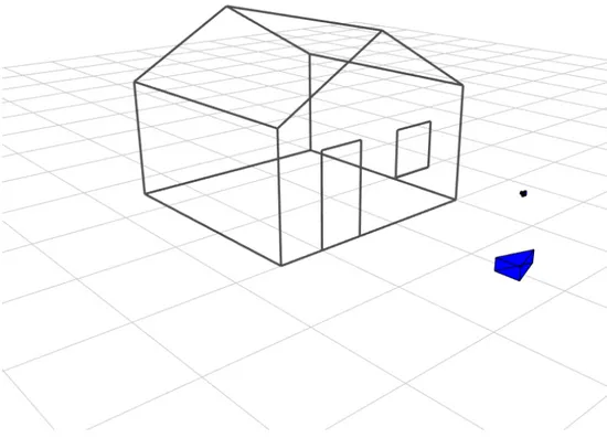
The figures 4.7 and 4.8 show the results of the implementation of a visual SLAM system.

4.3 Main challenges

Despite all progresses made by SLAM community research in the last decades, some problems still need solutions providing better performances. An overview of the main difficulties follows.

4.3.1 Computational Complexity

The SLAM problem is intrinsically a complex problem, due to the required estimation of a joint state composed of the robot pose and landmarks loca-tions. Computational efficiency becomes important for the scalability of the problem: the robot performing SLAM must be able to operate over an ex-tended period of time and to explore new spaces without letting the required memory grow unbounded [10].

(46)

Figure 4.7: Here is showed the simulated reconstruction of the landmarks of a house through a vision SLAM system

Figure 4.8: The figure shows the view of the camera performing vision

(47)

4.3.2 Data Association

Figure 4.9: Short term data association must recognise the measurements related to the same landmark in successive instants

As previously introduced, data association is one of the critical issues in SLAM implementations. It consists in associating the measurements to the correct landmarks. Outliers, which are false positive landmarks, can degrade the estimate, which in turn degrades the ability to individuate them [10].

The problem can be subdivided in two submodules:

Short term data association (figure 4.9): it deals with the fact that the sampling rate of the sensor is faster than the dynamics of the robot, thus making the last features observed very close to the current ones. Long term data association (figure 4.10): it is more complicate because

it aims at detecting and validating the loop closure events. A brute-force approach that tries to compare all new features with the older becomes numerically impracticable as the number of landmarks grows up. At the same time, a single wrong data association can induce divergence into the map estimate [6].

The data association problem becomes harder when the landmarks look different from different viewpoints [6].

4.3.3 Environment representation

Formerly, SLAM environment representation was supposed to hold as simple geometric primitives such as points, lines or circles. This hypothesis does

(48)

Figure 4.10: Long term data association must provide loop closure for land-marks that are being revisited

(49)

not hold in complex and unstructured environments like subsea, outdoor and underground.

The previously introduced (Chapter 2) characterization as feature-based maps and occupancy grid maps appears to be the simplest geometric environ-ment modelling in the 2D case. In the 3D case, the complexity is increased as vehicle motion and observation model must be generalized adding a dimen-sion. The situation is complicated by the fact that the assumption of a static world, that is often taken, does not always hold as sometimes landmarks are not fixed. The mapping in the long term or large spaces underlines this problem, since a change in the environments becomes more probable [10] [6]. Furthermore, when vision SLAM is employed, the question whether us-ing semantic or topological mappus-ing opens up; while topological mappus-ing is about recognising a previously seen place, the semantic mapping deals with classifying the place according to a pre-recorded semantic database [10]

4.3.4 New frontiers for SLAM

The development of new algorithms and the availability of more advanced sensors have always been the main trigger for the progress in SLAM. Applica-tions such as autonomous cars or augmented reality has taken off respectively due to progresses in LASER and vision systems [10].

New sensors in the vision field are now under study by research commu-nity:

Range cameras: they are light-emitting depth cameras that works ac-cording to different principles, such as structured light, time of flight, interferometry, or coded aperture. While structured light cameras work by triangulation and use different perspective illumination of an object to deduce his shape. This kind of camera is provided with his own light source, thus making them work in dark and untextured scenes.

Light-field cameras: they record not only the intensity of the light impacting the single pixel, but also the direction of the ray. Light-field cameras have different advantages with respect to standard cameras, such as depth estimation, noise reduction, video stabilization, isolation of distractors, and specularity removal. However, the manufacturing cost is responsible of their low resolution, still less than a megapixel in the commercially available ones.

Event-based cameras: they are basically different from standard cam-eras, because the images are not sent entirely in fixed frame rates, but

(50)

only the local pixel-level change is sent when a movement in the en-vironment occurs. This makes possible the increase of dynamic range, update rate and the decrease of power consumption, latency. The re-quirements of bandwidth and memory are also reduced [10].

(51)

Chapter 5 MATLAB implementation of

different SLAM technologies

In this chapter, the results of simulated implementation of SLAM through different technologies are showed. For this purpose, I exploited two different MATLAB toolbox:

Visual EKF-SLAM Toolbox: developed by Joan Sol`a in 2013, it imple-ments an EKF algorithm simulating a 3D environment

LIDAR EKF-SLAM Toolbox: developed by Tim Bailey and Juan Nieto in 2004, it can be used to simulate the implementation of an EKF algorithm in a 2D environment

The performance of SLAM is evaluated when different sensing technologies are exploited, though the same 2D context has been considered through executing the visual SLAM with landmarks and robot sensor placed in the same plane; in this way the problem can be approximated as a 2D one, such as LIDAR toolbox.

The chosen context is part of the corridor on the 3rd floor in Cesena Campus of the University of Bologna, shown in figure 5.1.

During the simulation, the robot follows a closed path (round) along the corridors. The rounds performed by the robot are 15 in each technology: the choice of this high number is made to simulate the crowd-sensing concept. If we imagine that every round corresponds to a different robot, then we can think of 15 different robots performing SLAM in successive times.

The results are finally reported in order to have a comparison between different technologies at different conditions.

(52)

(53)

5.1 Visual SLAM toolbox

The visual SLAM toolbox is an open source package that attempts to simu-late an EKF-SLAM algorithm in a given environment using a visual SLAM technology implementation.

Since it simulates a visual-SLAM technology, the measurement model of the system is characterized by the choice of the sensor, which is between the followings:

Omnidirectional camera omniCam with resolution 1280x800 Pinhole camera pinHole with resolution 640x480

The motion models available in the package are the following: A constant speed motion model constVel

A circular uniform motion model odometry

Regarding the landmarks that here can be implemented, the choice is between:

Points: through the call to the function, called thickCloister.m, which generates a cluster of landmarks geometrically distributed through a 3D square ring volume, as shown in figure 5.2.

Lines: through the call to the function, called house.m, which repro-duces the shape of a house, as shown in figure 5.3.

5.1.1 Default main script slamtb

The package main file is called slamtb.m and it can be viewed in Appendix A. It initializes the environment through the call to the function userDataPnt.m, in which the choice of the sensor and the landmarks distribution can be made by editing the code following the guidelines. The choice of line landmarks, instead of point ones, can be made calling the function userDataLin.m.

In userDataPnt.m, not only the settings of the robot and sensor installed on it can be edited, but also the simulation and estimation options, ranging from standard error of sensor and number of landmarks initialized by the algorithm, to the choice of the type of landmarks that the algorithm must recognize.

(54)

Figure 5.2: Simulation of landmarks as points in Visual SLAM toolbox

An important detail that will become important later to recreate the en-vironment, is that even though only one type of landmarks can be initialized for recognition by the algorithm, lines and points can both be implemented. This allows the realization of buildings which contains the landmarks that needs to be detected.

Once initialized the environment, the main structure of the algorithm is initialized, including robot, sensor, landmarks and raw data structures.

To get a graphic support, also figures structures for the real-time plotting of the SLAM estimation progress are initialized.

Once finished the initialization phase, a code is repeated periodically through the use of a for structure. It implements:

The motion of the robot

The estimation of landmarks and robot pose through an EKF algorithm The update of the visual information on SLAM estimate

(55)

(56)

5.1.2 Realization of the SLAM estimation in the

con-sidered scenario

Environment

As previously stated, the context that I want to simulate is different from the available ones; for this reason I have made some changes in the main functions and scripts.

The landmark type chosen is the point, so the initialization of environ-ment is done editing the script userDataPnt.m into the script userDataCor-ridor.m, which recreates the shape of the corridor and collocates the point landmarks where desired; this code can be seen in Appendix A. The point landmarks that I have chosen represent the edges, the corners and the doors. To realize the shape of the corridor, I have edited the function house.m to build a new function called Corridor Ing Ces.m (shown in Appendix A). According to some constants related to the shape of the corridor like height, length and width, this function builds the corridor as shown in 5.1.

The script also initializes the initial position and orientation of the robot and the sensor, together with several other parameters that are not here specified for coinciseness.

Motion

Assumed that the robot must realistically move inside the corridor, I have exploited the motion model odo3.m to this purpose: by default it changes continuously the direction of the robot, when recalled by the main loop, in order to realize a circle trajectory.

What I have done was editing the main loop in order to let it call the function odo3.m only when the robot is situated near the corners; only in that case his direction of motion should change

For this purpose, I realized a function called locate robot.m to locate the robot position and orientation inside the corridor; this information is returned and exploited by a script I realized called DetDir.m. Given the detected pose of the robot, it determines whether the direction of the robot must change or not. Both this codes are shown in Appendix A.

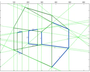
Visibility of landmarks

Since the SLAM technology in exam is a visual SLAM, the algorithm sim-ulated should not realistically be able to see the landmarks situated behind the walls. The observations are taken by the algorithm through a struct

(57)

Figure 5.4: The landmarks that the robot observe are the numbered ones, the other are not in LOS, so they are not visible

Figure 5.5: The view of the camera: it can be noticed that the not in LOS landmarks are not visible by the camera

(58)

called Obs which has a field called vis that flags if a landmark observation is possible or not.

To exploit this field, I have implemented a script, called DetVisLmk.m (it can be viewed in Appendix A), inside the function CorrectKnownLmk.m, which is called inside the main loop to correct the landmarks position ac-cording to the new observation; the script uses the geometrical information to set as not visible the landmarks not in LOS. In figures 5.4 and 5.5

Position estimation RMSE calculation

To have a precise idea of the behaviour of the algorithm, I have written a script called calc RMSE : it performs the calculation of the RMSE of both the robot pose (5.1) and landmarks (5.2) position once a lap. This code is showed in Appendix A. RM SE(xn) = Pn+N n=1 (xn− ˆxn)2 N (5.1) RM SE(mn) = PL i=1(m i n− ˆm i n)2 L (5.2) where

N is the number of time steps for each lap

L is the number of landmarks discovered until the instant n Configuration file

The main parameters, which I have modified to perform different simulations, have been initialized in a configuration script called configSLAM.m. It can be viewed in Appendix A.

Inside this script, I grouped the main parameters, such as:

CHOICE 2D 3D: decides whether the sensor must be placed in the same plane of the landmarks

N LOOPS: decides the number of loops that the robot must do around the corridor

NLOOPFRAME: number of time steps (also called frames) necessary to perform a single loop

(59)

NLMKS ROBOT : number of landmarks that must be initialized by the SLAM algorithm

PIX ERROR STD: standard deviation of pixel recognition of the cam-era sensor (it sets the accuracy with whom an object is localized in the right pixel by the camera)

POS STD: standard deviation of the robot motion error, it is set equal to 10 cm in x and y axes and equal to 0 in z axis

Sim Corr: decides if the environment to simulate must be a corridor In the initial phase, I have also simulated other environments using the default landmarks generating functions of the toolbox, to realize scripts that reproduce an environment according to the following parameters:

KIND LMK : it sets if the landmarks have to be represented as points or lines

KIND SENSOR: it sets the kind of sensor (omnidirectional camera and pinhole camera are available)

N ROBOTS : it sets the number of the robots

5.1.3 The result of simulations

Given the introduced and edited codes, I have proceeded to simulate several times the implemented scenario; each time I changed the pixel standard error parameter of the camera to observe the different behaviour of the estimate as a function of this parameter.

The selected values of the error standard deviation varies between the following values, grouped in a vector:

pix err std = (0.1, 1, 5, 10, 20, 30, 50)px

I have also made the choice of keeping low the value of the standard deviation of the robot position error (10 cm in both x and y axis, 0 cm in z axis) and to not consider the z axis error in RMSE calculation; the reason is that I wanted to simulate a 2D scenario, similar to the one of LIDAR SLAM implementation, which will be explained in the next section.

The number of landmarks initialized by the algorithm has been kept as low as possible in order to make the algorithm faster.

The results of the simulations are summarized in the following tables ( 5.25.1) and figures (5.6,5.7,5.8,5.9,5.10,5.11,5.12)

(60)

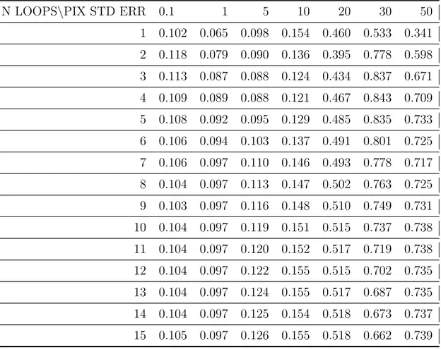
Table 5.1: Position robot RMSE in metres referred to different number of loops and pixel standard deviation

N LOOPS\PIX STD ERR 0.1 1 5 10 20 30 50 1 0.102 0.065 0.098 0.154 0.460 0.533 0.341 2 0.118 0.079 0.090 0.136 0.395 0.778 0.598 3 0.113 0.087 0.088 0.124 0.434 0.837 0.671 4 0.109 0.089 0.088 0.121 0.467 0.843 0.709 5 0.108 0.092 0.095 0.129 0.485 0.835 0.733 6 0.106 0.094 0.103 0.137 0.491 0.801 0.725 7 0.106 0.097 0.110 0.146 0.493 0.778 0.717 8 0.104 0.097 0.113 0.147 0.502 0.763 0.725 9 0.103 0.097 0.116 0.148 0.510 0.749 0.731 10 0.104 0.097 0.119 0.151 0.515 0.737 0.738 11 0.104 0.097 0.120 0.152 0.517 0.719 0.738 12 0.104 0.097 0.122 0.155 0.515 0.702 0.735 13 0.104 0.097 0.124 0.155 0.517 0.687 0.735 14 0.104 0.097 0.125 0.154 0.518 0.673 0.737 15 0.105 0.097 0.126 0.155 0.518 0.662 0.739

(61)

Table 5.2: Position RMSE in metres referred to different number of loops and pixel standard deviation

N LOOPS\PIX STD ERR 0.1 1 5 10.000 20.000 30.000 1 0.127 36.457 90.959 0.220 1.145 35.097 2 0.125 0.093 85.537 0.162 0.455 72.699 3 0.103 0.082 0.076 0.110 0.581 18.031 4 0.109 0.102 0.109 0.168 0.598 1.412 5 0.101 0.099 0.116 0.188 0.574 1.240 6 0.104 0.099 0.128 0.189 0.587 1.121 7 0.105 0.105 0.145 0.194 0.553 0.997 8 0.100 0.089 0.117 0.154 0.604 0.884 9 0.107 0.090 0.135 0.171 0.595 0.862 10 0.108 0.085 0.125 0.168 0.575 0.752 11 0.109 0.089 0.120 0.157 0.564 0.716 12 0.112 0.090 0.128 0.163 0.542 0.672 13 0.115 0.096 0.153 0.190 0.521 0.612 14 0.114 0.089 0.122 0.142 0.592 0.650 15 0.117 0.087 0.122 0.151 0.573 0.626

(62)

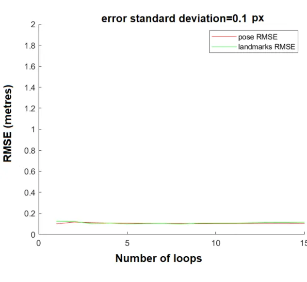
Figure 5.6: Result of simulation considering a error standard deviation value equal to 0.1

(63)

Figure 5.7: Result of simulation considering a error standard deviation value equal to 1

(64)

(65)

(66)

(67)

(68)

Given these results, some main considerations can be done:

The position estimation error of both landmarks and robot grows up with the pixel standard error

If we consider a camera sensor conditioned by a large pixel standard deviation error (up to 50), if the number of laps is sufficiently large, the robot localization performed by the algorithm still gives good results. With the increase of the number of laps travelled by the robot, the

(69)

the concept of crowd-sensing is useful in the localization of landmarks, whose positions are initially completely unknown. A remarkable ex-ample is shown in 5.2 in the column corresponding to a pixel standard deviation equal to 30: despite an initially bad landmarks position esti-mation, after few laps the system recovers.

Since the pose of the robot is initially well known, crowd-sensing does not make a significant difference in his localization performance. This could be ascribed to the ”loop closure” phenomenon of SLAM.

5.2 LIDAR SLAM toolbox

The LIDAR SLAM toolbox is an open source package that attempts to simu-late the EKF-SLAM algorithm in a given environment using a LASER SLAM technology implementation.

This package is implemented in a quite different way than the previous one. Here the main script, called execute ekf, loads a set of predefined land-marks and waypoints. The latter are the points through which the robot is supposed to move.

After the data load, the core function of the package is called; the func-tion in exam is named ekfslam sim and it performs the entire simulafunc-tion of the algorithm using the input data that not only include landmarks and waypoints, but also parameters of the corridor that has to be simulated.

5.2.1 The main function ekfslam sim

The first thing that the function does is setting the configuration parameters of the problem through the script configfile; this script can be viewed in Appendix B. Then the environment is plotted with a 2D representation.

After this, the main loop starts running and executing the following op-erations at every cycle:

the motion control is computed, together with the associated noise the prediction and update steps of the EKF are computed

(70)

5.2.2 Realization of the SLAM estimation in the

con-sidered scenario

Since this code package is less complicate and advanced than the previous one, here I limited my contribution in adapting the data saved after the execution of the vision SLAM algorithm, in order to let the robot follow the same path; specifically, during the execution of visual SLAM code, I recorded with a fixed time step the positions of the robot during the path and used them to define the waypoints given as input to the LIDAR SLAM code.

The meaning given to landmarks is different from that given in Visual SLAM: here they are used to emulate wireless access points (AP) supposed deployed in the corridor. In this way, by properly setting the parameters observation model (i.e., noise level), it is possible to simulate a Wi-Fi SLAM technology using a software initially designed to simulate a LIDAR-based SLAM system.

A similar reasoning can be made by setting very low error standard de-viation parameters for angle of arrival and distance estimations, in order to simulate a mmW/UWB-based SLAM.

The results of the next subsection are obtained by making two hypotheses:

The interaction between APs and robot brings a distance measurement through the analysis of the received signal strength (RSS)

Through the installation of an array of antennas is possible to deduce a signal angle of arrival measurement.

(71)

Figure 5.13: Simulated scenario: the landmarks are indicated in blue, while the waypoints are the green dots

The RMSE related to robot pose and landmarks position estimate is calculated through a script called calc RMSE lidar.

The parameters are set in the script called configfile; it is used to set the following parameters among the others:

Position: it is a two-dimensional vector who defines the initial position of the robot through x and y coordinates expressed in m

Orientation: it defines the initial orientation of the robot in rad sigmaV : it defines the standard deviation of the robot speed referred

in m/s

sigmaG: it defines the standard deviation in angle of motion referred in rad

MAX RANGE: it defines the maximum detection range of landmarks expressed in metres

Simultaneous Localization and Mapping Technologies

ALMA MATER STUDIORUM - UNIVERSIT `

A DI BOLOGNA

CAMPUS DI CESENA

Scuola di Ingegneria e Architettura

CORSO DI LAUREA MAGISTRALE IN

Ingegneria Elettronica e Telecomunicazioni per l’Energia

SIMULTANEOUS LOCALIZATION AND

MAPPING TECHNOLOGIES

Elaborato in

Reti di Sensori Wireless per Monitoraggio Ambientale

Relatore

Chiar.mo Prof. Ing.

DAVIDE DARDARI

Correlatore

Dott. Ing.

NICOL `

O DECARLI

FRANCESCO GUIDI

Presentata da

NOUR NAGHI

Sessione III

Anno Accademico 2017-2018

Contents

Abstract

Keywords

List of Abbreviations

Chapter 1

Introduction

Chapter 2

Mathematical tools for the

study of dynamic physical

systems

2.1

Representation of a physical dynamic

sys-tem

2.2

Bayesian filters

2.3

Kalman filters

2.4

Extended Kalman filters

2.5

Particle filters

Chapter 3

Localization and mapping in

dynamic physical systems

3.1

The mapping problem

3.2

The localization problem

3.3

The SLAM problem

Chapter 4

State of the art related to the

SLAM problem

4.1

Anatomy of a SLAM system

4.1.1

Back-end

4.1.2

Front-end

4.1.3

Odometry

4.1.4

Sensors in SLAM

4.2

The main SLAM technologies

4.2.1

SONAR SLAM

4.2.2

RADAR SLAM

4.2.3

LASER SLAM

4.2.4

Visual SLAM

4.3

Main challenges

4.3.1

Computational Complexity