Dual Energy CT: an alternate approach for metal artefact correction

(1)

Alma Mater Studiorum

_{· Universit`a di Bologna}

Scuola di Scienze

Dipartimento di Fisica e Astronomia Corso di Laurea in Fisica

Dual Energy CT: an alternate approach for

metal artefact correction

Relatore:

Prof. Maria Pia Morigi

Correlatore:

Dott. Fauzia Albertin

Dott. Rosa Brancaccio

Presentata da:

Valentino Recaldini

(2)

(3)

L’argomento centrale di questa tesi è lo studio di una correzione per uno dei più di↵usi artefatti legati alla tomografia a raggi X: il metal artefact. Questo tipo particolare di artefatto compare quando oggetti particolarmente radiopachi—ad esempio chiodi in acciaio o ossa—vengono acquisiti insieme a materiali poco assorbenti, come ad esempio la carta o i tessuti molli. In particolare, il metal artefact interferisce con la corretta ricostruzione dell’og-getto studiato a partire dalle sue proiezioni, ed esistono diversi approcci per correggerlo o quantomeno ridurlo. Tra questi c’è la Dual Energy Computed Tomography in cui l’oggetto viene acquisito con due diversi spettri energe-tici. In questa tesi si cerca una formulazione matematica per la correzione ottimale dell’artefatto.

Si sono utilizzati due fantocci—uno di Plexiglas e uno di legno—che sono stati precedentemente modificati per consentire l’inserimento di oggetti me-tallici. I fantocci sono stati acquisiti con due diversi spettri policromatici a raggi X opportunamente filtrati. Si sono scelti le correnti e i tempi di esposi-zione cosicch´e entrambe le acquisizioni (a basso e ad alto voltaggio) avessero una intensit`a rilevata dal detector simile.

Per ciascun fantoccio, le ricostruzioni tomografiche ottenute sono state combinate con di↵erenti parametri e poi analizzate sia qualitativamente che quantitativamente per stimare la correzione del metal artefact e la perdita di dettaglio all’interno di materiali poco assorbenti.

(6)

(7)

Abstract

This thesis focuses on the problems caused by the metal artefact, one of the artefacts intimately related to Computed Tomography (CT). They ap-pear when radiopaque objects are acquired alongside weakly absorbing ma-terials and interfere with the correct reconstruction from raw CT images. Several approaches to fix this problem exist, one being Dual Energy CT (DECT), where the object is scanned at two di↵erent voltages. In particular, in this thesis, a mathematical formulation for the optimal artefact correction is sought.

Two phantoms—a Plexiglas one and a wood one—were adjusted to fit metal objects for the study before they were acquired at two di↵erent volt-ages with opportune X-ray spectrum filters. The currents and the times of exposure were chosen so as to have a similar detected intensity in both acquisitions.

For each phantom, the reconstructed CT sets were processed together with di↵erent parameters and then analysed both qualitatively and quanti-tatively to estimate the metal artefact correction and the detail loss within weakly absorbing materials. The quantitative analysis is performed with Michelson contrast.

(8)

(9)

Introduction

The metal artefacts are a well-known drawback of Computed Tomography (CT). They a↵ect CT reconstruction where materials with very high atten-uation coefficients are acquired alongside weakly absorbing objects. The reasons behind its existence lie in the physics which underpins the interac-tion between X-rays and matter and in the reconstrucinterac-tion algorithm used (Filtered-Back-Projection, or FBP).

There are several methods to correct the metal artefacts. One of them is Dual Energy Computed Tomography (DECT), where an object is acquired at two di↵erent voltages (and thus with two di↵erent photon spectra) and both raw CT sets are combined together to obtain specific results: e.g. metal artefact correction, material-based decomposition or enhanced image quality. The thesis work revolved around DECT and the quest for the optimal parameter for metal artefact correction. In particular, the relation between contrast and metal artefacts was studied in depth and corrective parameters were extracted from the theoretical background. An interval of values within which there is a remarkable metal artefact reduction was found.

An experiment was set up for a Dual Energy sequential acquisition of two ad hoc phantoms with one of the tomographs of the University of Bologna’s Department of Physics and Astronomy. The voltages were 70 kV and 120 kV. The high voltage beam was filtered with a 2 mm copper plate. The images obtained from the reconstructions were combined with the corrective parameters and then studied both qualitatively and quantitatively to verify the contrast-based corrections.

This thesis is structured in three chapters. The first provides a theoreti-cal background on the physics underpinning X-rays and Computed Tomog-raphy and their applications. Moreover, the importance of X-ray filtration is stressed, and the metal artefacts are explained in depth. The chapter ends with an overview on DECT.

The second chapter explains the experiment. First, the filter choice is explained, and the formula used is studied extensively. Then, the appara-tus and the Plexiglas and the wood phantoms are shown. Lastly, the data

(10)

acquisition parameters are reported.

The last chapter provides the experimental results of the phantoms, cor-roborated with reconstructed images, line profiles and tables.

The thesis ends with the conclusions and an appendix on the calculation of the uncertainties of the parameters studied.

(11)

Chapter 1 Theoretical Background

1.1 A Brief Introduction to X-Rays

X-rays are electromagnetic radiation whose energy usually ranges from 100 eV to about 100 keV, although photons with energy higher than 100 keV are still considered X-rays. They were first discovered by Wilhelm Conrad Roentgen in 1895. Additional experiments led to the conclusion that the interposition of various materials of di↵erent thickness between the source and the X-ray detector reduces the intensity of X-radiation.

1.1.1 X-ray Interaction with Matter

The physical law which expresses the attenuation of monochromatic X-rays when they travel through matter is

I(E) = I0(E)e R

Lµ(E,l)·dl (1.1)

where I and I0are the final and the initial intensities of X-radiation, E is the

energy of the X-rays and L is the path through which they have travelled to pass the object. Please note that L is not arbitrary and is a straight line if there was no di↵raction, di↵usion or photoelectric e↵ect. Moreover, µ is the attenuation coefficient, which is a function of energy and also depends on the material atomic number and density and thus is not constant. The equation (1.1) is often called the Beer-Lambert law, the Beer-Lambert-Bouguer law or Beer’s law.

The attenuation coefficient µ can be expressed as a function of the atomic attenuation coefficient µa [1],

µ = ⇢NA

(12)

where NA is the Avogadro constant (⇠ 6.022 · 1023 mol 1), A is the atomic

weight (in g mol 1_{) and ⇢ is the density of the material. The atomic}

attenu-ation coefficient is an atomic cross section and represents the probability of interaction between a photon and an atom of the material.

For energy values lower than 1.022 MeV, the attenuation coefficient is due to incoherent (or Compton) and coherent (or Thomson-Rayleigh) scattering and the photoelectric e↵ect, and µa can be written as a sum of the cross

sections,

µa= ⌧a+ a,C + a,R (1.3)

where ⌧a, a,C and a,R are, respectively, the atomic cross section due to the

photoelectric e↵ect and Compton and Rayleigh scattering.

The mass-energy equivalence for an electron-positron system is E⇤ = 2mec = 1.022 MeV, and thus, for energy values greater than E⇤, µ is also

due to pair production. Under this hypothesis, µa can be expressed as [1]

µa = ⌧a+ a,s+ a,pp (1.4)

where a,pp is the cross section due to pair production and a,s = a,C+ a,R.

The contribution of each cross section varies with energy and the atomic number (Z), and there are regions where one is predominant whereas the others have less or no influence over the result, as shown in Fig. 1.1.

Fig. 1.1: The relative importance of each cross section in µa.

For energy values lower than about 1 MeV, the attenuation coefficient is a non-continuous piecewise decreasing function of energy in R+_{. Its}

dis-continuities are caused by particular e↵ects called K-edge, L-edge or M-edge (Fig. 1.2). These edges are generated by X-rays with enough energy to free electrons in the inner K, L or M shells of an atom when absorbed. After a minimum of µ, it increases and tends to a horizontal asymptote due to pair production (Fig. 1.3).

(13)

Fig. 1.2: The mass attenuation coefficient, or µ_⇢, for silver (Z = 47), plotted as a function of energy in the range [10 3, 0.5] MeV. Please observe the peaks corresponding to the edges. From left to right: LIII, LII, LI and K edges. The images come from NIST database [2].

Fig. 1.3: The lead attenuation coefficient as a function of photon energy, expressed by (1.2) and (1.4).

(14)

1.1.2 X-ray Production

The employment of an X-ray tube is the simplest and most common way to produce X-radiation. X-rays are generated in cone beams, although the application of one or more collimators can yield fan beams.

Fig. 1.4: A reproduction of an X-ray tube without a collimator.

The diagram of an X-ray tube with a tungsten anode is depicted in Fig. 1.4. The filament (cathode) is heated by an electric current and releases electrons which then are accelerated towards the target(anode), and their collision with it produces the X-rays. It is therefore mandatory to have a vacuum inside the tube. X-ray tubes are often enclosed in lead protective sleeves to avoid the dispersion of unwanted radiation.

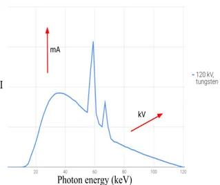
The X-ray spectrum (Fig. 1.5) is composed of two parts: braking radi-ation, which is at the origin of the continuous spectrum and is also called Bremsstrahlung, and a few peaks, which are the characteristic X-rays and depend on the target material. There are two main factors which modify the spectrum: e.g. the voltage, which varies the spectrum shape (maximum photon energy and the X-radiation intensity), and the current, which linearly changes the X-radiation intensity.

The energy values of the characteristic X-rays depend on the target ele-ment and are related to transition energy, which is the di↵erence in binding energy of the freed electron and of the one that takes its place, or

E = h⌫ = Eb,f Eb,n (1.5)

where Eb,f and Eb,n are respectively the values of the energy of the freed

electron and the new one, and Eb,f < Eb,n, ⌫ is the photon electromagnetic

(15)

Fig. 1.5: An example of an X-ray spectrum produced by a tungsten target at 120 kV. An increment of the current (mA) leads to a linear increase of the intensity (_"), and the voltage (kV)) modifies the spectrum shape and the intensity (_%). The spectrum was generated with Siemens’ simulator [3].

X-rays can also be produced with a synchrotron, and in this case they would be mono-energetic, or monochromatic, and come in parallel beams, which is useful for many applications. Unfortunately, this technology is not portable and rather expensive, and therefore polychromatic X-ray tubes are generally preferred.

1.2 Filters for X-ray Tubes

Beam hardening

When a polychromatic X-ray beam travels through a generic material, the spectrum shape changes according to (1.1), and this e↵ect is called beam hardening. Since the attenuation coefficient is much higher when the energy of the photons is low, less energetic photons are completely absorbed by matter, which implies that the resulting X-ray beam has a higher mean energy value, though the total flux of photons is lower.

Filters

Filters are often employed to optimise the X-ray spectrum shape and the beam intensity. They are convenient in diagnostic applications, namely ra-diography and Computed Tomography in medical physics. Indeed, photons with energy lower than about 10 keV are completely absorbed by the patient

(16)

and thus do not reach the detector and irradiate him/her without any benefit while being a potential source of harm. The application of a filter between the tube and the patient modifies the beam and therefore allows either to reduce or provide a better use of the absorbed radiation.

An X-ray filter is an object with a simple geometry and is made of a homogeneous material whose thickness, density and attenuation coefficients are known. Therefore, Beer’s law (1.1) can be further simplified. Let x be the material thickness and E the energy value. Then, (1.1) can be expressed as

I(E) = I0(E)e µ(E)x= I0(E)e

µ(E)

⇢ ⇢x (1.6)

where ⇢ is the material density. The value µ_⇢ is frequently defined as the mass attenuation coefficient. It is therefore feasible to calculate the exact shape of the filtered spectrum. An example of how filtration a↵ects the original spectrum is shown in Fig. 1.6.

(a) 70 kV spectrum, unfiltered and fil-tered with 0.1 mm thick silver plate.

(b) 70 kV spectrum filtered with silver plates of di↵erent thickness: 0.75 mm, 1 mm and 1.5 mm.

Fig. 1.6: Beam hardening can be graphically observed by comparing the unfiltered spectrum in (a) and any filtered spectrum in (b). Silver K-edge is observed at 25.51 keV [2]. (Unfiltered spectrum generated from [3].)

1.3 Application of X-rays

For their high penetrating power, X-rays have been employed in several di-agnostic procedures, e.g. radiography and Computed Tomography.

In medical physics, the tube voltage is generally between 10 kV and about 140 kV [4] because higher photon energy leads to lower contrast in the pro-cessed images due to the attenuation coefficient behaviour in this range, and low-energy photons are completely absorbed by the patient. The equation

(17)

(1.3) can therefore be used to describe µa because pair production is not

involved.

While in medical physics filters are widely employed (see paragraph 1.2), in some cultural heritage applications it is best not to apply them. Indeed, their use could potentially erase information carried by low-energy photons when some materials with very low attenuation coefficients are analysed, as they tend to become transparent to X-rays when the voltage is too high. However, if radiopaque materials are the main focus of the study, filters are applied to increase the mean energy of the X-ray beam.

The simplest radiography machine is composed of two elements: an X-ray tube to produce X-radiation and a detector, be it a photographic plate or a digital sensor, which must be aligned. This system can be further improved by the interposition of one or more collimators right after the tube, before the detector or in both positions. A filter can be applied between the tube and the patient.

A tomograph (Fig. 1.7) is the natural evolution of a radiography machine and is used to obtain the three-dimensional structure of the studied objects. Indeed, the only variation from it is that either the tube-detector system or the patient—or the object—needs to rotate so as to acquire di↵erent radio-graphies to reconstruct a three-dimensional image. In medical physics, the system rotates to ensure the patient’s safety. On the other hand, in cultural heritage it is feasible to rotate the object without particular risks.

(18)

1.4 Computed Tomography

Computed Tomography, often addressed as CT, is one of the applications of X-rays and was first performed by Hounsfield in 1971. With this technique, it is feasible to analyse the inside of an object without actually opening it. Therefore this approach is non-invasive.

In the case of parallel and non-di↵racting X-ray beams, Computed To-mography consists in the resolution of an inverse problem. Indeed, given q two-dimensional projections P✓(t) of a three-dimensional object f (x, y, z),

its three-dimensional structure is sought and has to be reconstructed. For simplicity, z will be constant. Therefore, f (x, y, z) = f (x, y) and the projec-tion are one-dimensional. It is feasible to reconstruct the three-dimensional object by using a set of f (x, y) at di↵erent z.

Fig. 1.8: A sketch of the object f (x, y). Please note that the coordinates t and s and the coordinates x and y at the angle ✓.

The mathematical problem was solved by Radon in 1917 with the intro-duction of his transform [5]

R(f (x, y)) = P✓(t) = Z (✓,t)line f (x, y)ds = Z ₁ 1 Z +1 1

f (x, y) (x cos ✓ + y sin ✓ t)dxdy

(1.7) and anti-transform R 1(P✓(t)) = 1 (2⇡)2 Z ⇡ 0 d✓ ✓Z +1 1 1 x cos ✓ + y sin ✓ t @P✓(t) @t dt ◆ (1.8)

(19)

where s moves along the beam direction. Furthermore, the subscript (✓, t) specifies that it holds for each ✓ and t. The variables t and s are related to x and y by _ t s =  cos ✓ sin ✓ sin ✓ cos ✓  x y (1.9)

The variables and objects are shown in Fig. 1.8.

The equation (1.8) yields f (x, y), which is the solution. Moreover, in the CT case, from (1.1), f (x, y) is related to µ(x, y) by

Z (✓,t)line f (x, y)ds = ln ✓ I0,z(t) I✓,z(t) ◆ = Z (✓,t)line µ(x, y)ds (1.10)

where the subscripts ✓ and z specifies that it refers to the angle of acquisition ✓ and the height z, and dl from (1.1) is ds. I0,z(t) is the X-ray intensity

measured when no object is interposed between the source and the detector. It follows that each of the aforementioned projections is a set of line integrals [5]. R(f (x, y)) is often defined as a sinogram (P✓(t), 0  ✓ < 2⇡).

Unfortunately, with a finite—and thus discrete—number of projections, which correspond to the angles of acquisition in (1.7), and positions, which are points along the t-axis of the sinogram, Radon’s approach to the recon-struction of f (x, y) is not permitted because the equation (1.8) may be diver-gent due to one or more discontinuities of the derivative inside the integral. The concept of sinogram, however, is still useful during the reconstruction process.

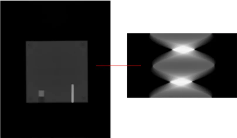
Fig. 1.9: (Left) a projection on which the formula (1.10) was performed. (Right) a sinogram. The arrow connects the j-line to its place within the sinogram Sj.

Moving upwards or downwards in the sinogram will result in the j-line of another projection in the dataset.

(20)

Let q be the number of finite projections, m their height and n their width (in pixels), and let k, j and i be integers which can vary between 0 and respectively q 1, m 1 and n 1. Then the element Sj(i, k) of a sinogram

can be defined as the pixel corresponding to the opportune coordinates i and j of the projection k. Therefore, the sinogram Sj (Fig. 1.9) is the collection

of all the possible pixels i and k for a selected j, or, in other words, the orderly evolution of the j-line when the object rotates and thus the angle (k) varies.

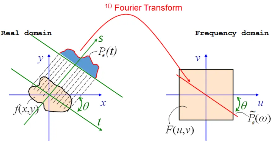
An important step in the solution of the real computed tomography prob-lem is Fourier’s slice theorem [5]. Let f (x, y) be an image, P✓(t) its parallel

projection and ✓ the angle at which it was taken (Fig. 1.10). Then the one-dimensional (1D) Fourier transform of P✓(t) yields the values of the

two-dimensional (2D) Fourier transform of f (x, y), F (u, v), along the line which forms the same ✓ with the u-axis in Fourier’s frequency space while passing through the coordinate origin.

Fig. 1.10: Fourier’s slice theorem.

It may seem that the solution to the problem is close and that only a 2D Fourier anti-transform from Fourier’s space back to the real domain is needed. However, it is important to understand that frequencies around the origin of the coordinates in Fourier’s space are more densely packed, as shown in Fig. 1.11a. The application of a filter (traditionally a ramp filter, as shown in Fig. 1.11b) helps to even out the di↵erences in frequency density in Fourier’s space, which translates into a better reproduction of the edges when the 2D Fourier anti-transform is performed. Nowadays, other filters are employed to achieve better results at edge preservation without degrading the Signal to Noise Ratios.

(21)

anti-(a) An example of the fre-quency distribution in Fourier’s space.

(b) The ramp filter originally employed in the FBP algorithm. Its equation is f (x) =_{|x| if}

1

2⌧ < x < 1

2⌧ [5], where ⌧ is the sampling

interval (pixel size), and the ends of the inter-val are obtained through Nyquist’s theorem.

Fig. 1.11: In (a), the further away from the centre, the more scattered the points are, which implies that their density is lower. The application of the ramp filter (b) in (a) helps to even out this density di↵erence.

transform is reported below.

f (x, y) = Z +1

1

Z +1

1

F (u, v)ei2⇡(ux+vy)dudv (1.11)

The equation (1.11) is the solution of the problem. However, one can fur-ther improve it by applying Fourier’s slice theorem, (1.9) and the following substitutions:

u = ! cos ✓ (1.12a)

v = ! sin ✓ (1.12b)

After a few mathematical manipulations, the solution becomes

f (x, y) = Z ⇡ 0 d✓ ✓Z +1 1 ( eP✓(!))|!|ei2⇡td! ◆ (1.13)

where eP✓(!) is the 1D Fourier transform of the parallel projection P✓(t) at a ✓

angle and_{|!| is the filter in Fourier’s space. Note that the integral inside the} parentheses is the 1D Fourier anti-transform and its result is then integrated over the angles between 0 and ⇡ (⇡ because the beam is parallel).

(22)

The equation (1.13) is the base of the Filtered-Back-Projection algo-rithm [5] and is the backbone of tomographic reconstruction. It implies that each projection must be filtered in Fourier’s frequency space and then back-projected in the real domain, where the value of each filtered back pro-jection must be assigned to the whole line of integration and this procedure has to be repeated for all the projections at di↵erent angles. At the end, a slice is obtained with real values for each pixels. However, negative values has no physical meanings, and therefore they are set to 0 at the end of the FBP algorithm.

(a) (b)

Fig. 1.12: Both images have been computed with the same 16 projections of a Plexiglas phantom. (a) was obtained with the FBP procedure, while in (b) the filter was disregarded. Note how unfocused (b) is with respect to (a) and the star artefact in (a): the phantom shape is hard to understand even when the edges are preserved.

The equation (1.13) is valid provided the acquisition angles are compa-rable with the detector pixel width; otherwise, a result like Fig. 1.12a can be found. This reconstruction artefact is often called star artefact. To un-derstand the importance of an adequate number of angles and the filter, Fig. 1.12b is shown. The object in Fig. 1.12b is surrounded by a halo. Furthermore, it is hard to detect its boundaries in either image.

Reconstruction with di↵erent beam geometries is feasible, although some corrections must be taken into account due to changes in geometry (e.g. mag-nification) and thus di↵erent algorithms and generally more computational power are needed. This is especially true when the beam is conic because all the entire projections—and not only a set of positions at a fixed height z—are needed to reconstruct a single axial slice. Indeed, each element of the

(23)

object is not bounded to said set at a fixed z due to the beam shape. This procedure must then be repeated to obtain the whole object.

The best solution to the three-dimensional cone beam reconstruction problem was found by Feldkamp, Davis and Kress (and is called FDK al-gorithm) [5]. Their algorithm is still based on FBP, but the back-projection is computed in three dimensions.

1.5 Metal Artefacts

(a) (b) (c)

Fig. 1.13: Some metal artefacts due to an aluminium (big) cylinder and a steel (small) one, both inserted in a wood phantom. Around the small cylinder, the sig-nal has practically been erased, while in the other areas it has only been decreased. The grey level range has been set to be the same for all the pictures.

The metal artefact (Fig. 1.13 and Fig. 1.14) is one of the main inherent drawbacks of FBP algorithms. Its name arises from its frequent appear-ance in medical CT when metal objects are scanned alongside less absorbing materials like soft tissues.

Please note how multiple highly absorbing objects can produce much higher artefacts when combined, as shown in Fig. 1.13b and 1.13c, and how much more absorbing the cylinders are in comparison to the surrounding wood. The di↵erence in absorption can be seen better in Fig. 1.14 as the grey level range varies. The white lines around the artefact region is also caused by the metal artefact.

There are two main reasons for its existence. The first is inherent to physics and the theory behind the Back-Projection procedure. If A and B are two di↵erent objects in a set of projections, A being much more absorbing than B, and µA and µB are their attenuation coefficients, then the signal

(24)

(a) (b) (c)

Fig. 1.14: A slice of a Plexiglas phantom, with the same cylinders as Fig. 1.13, observed at di↵erent floating point grey levels: (a) range [0,1]; (b) range [0,5.5], (c) range [0,11].

produced by B is hidden by that of A. Physically, when the X-ray beam travels through A, it is hardened by Beer’s law (1.1), the lesser energetic photons being absorbed by matter. Then, weakly absorbing objects like B become transparent to the beam and do not hinder its journey, which implies that they are not detected. In this scenario, data cannot be retrieved because they are not acquired in the first place. Furthermore, because of the FBP algorithm, since the value of each pixel is assigned to the line (or back-propagated) and the projections are summed and since µA >> µB, the data acquired from A weights more than and hides B, even if A is present in few projections.

The second reason is due to the properties of the filter used in the FBP al-gorithm. Indeed, its employment produces negative values around the edges to aid their preservation in the reconstructed images. Highly absorbing mate-rials, however, have higher absolute values even when they are negative, and therefore they ”dig” around their edges, partly erasing the signal produced by lesser absorbing objects, as shown in Fig. 1.13 and Fig. 1.14a.

This problem has been addressed multiple times [6] and there are several approaches to correct it. Generally, they can be separated into two main categories—those employed after the acquisition, and those before.

An example of a post-acquisition method is an algorithm which lowers the grey levels of the highly absorbing objects within the projections before the reconstruction so as to diminish the defects of the FBP algorithm. The main drawback of this method is that it is generally not easy to detect the right regions of the images where the highly absorbing materials are only

(25)

when a set of (1.10) is known since two objects of di↵erent thickness might lead to the same value when the integral is performed.

An example of a pre-acquisition method is the Dual Energy Computed Tomography, which will be discussed later and on which this thesis will focus.

1.6 Dual Energy (Computed) Tomography

Dual Energy (Computed) Tomography, often shortened as DECT, is an ap-plication of CT. It consists of the acquisition of two sets of the raw CT images at two di↵erent energies or, in most cases, voltages (high and low) [1].

Soft tissues, paper and wood are weakly absorbing materials and progres-sively become transparent when the energy of the photons is increased. On the contrary, bone-like objects or metals are highly absorbing materials and thus require higher photon energies to be successfully penetrated by a suffi-cient amount of photons. Furthermore, the di↵erence in absorption between the materials lessens as energy increases. Therefore, the lower voltage set yields a better contrast within weakly absorbing objects, whilst the higher voltage set provides a better reconstruction with fewer and less-severe metal artefacts. Moreover, the contrast within the high voltage images is over-all lower. This implies that, theoreticover-ally, it should be possible to correct the metal artefacts while still preserving the details of the weakly absorbing materials.

DECT is often used in medical physics to enhance the image quality, correct metal artefacts (e.g. when a patient has metallic implants [7]), or perform a material-based decomposition [8] on the reconstructed images so as to obtain two new sets with one material each.

Fig. 1.15: Bragg’s di↵raction in a multilayer lattice crystal.

Dual Energy Computed Tomography can be obtained with the aid of a synchrotron, which yields monochromatic X-rays or by employing a pyrolytic graphite target to di↵ract polychromatic X-rays in mono-energetic rays at

(26)

di↵erent ✓ angles by rotating the crystal. This is shown by Bragg’s law,

2dsen✓ = n (1.14)

where d is the interplanar distance between two lattice planes (as shown in Fig. 1.15), ✓ the beam incident angle, the wavelength and n a positive integer. The latter approach is used for Dual Energy mammography and radiography in cultural heritage applications [9].

Dual-energy Tomography with (polychromatic) X-ray tubes is feasible and filters are often employed [4] [10] to modify the spectra and perform it. Indeed, the usage of a filter produces a change in the X-ray spectrum (Fig. 1.6), and thus it is feasible to obtain two X-ray beams whose spectra have the least overlap possible. This is of utmost importance because, if a DECT acquisition with a small overlap is performed, the scans carry di↵erent details. On the contrary, a large overlap would yield similar information in both acquisitions and would also entail an inefficient use of the X-radiation dose to which the object or the patient has been exposed. Parameters such as the current and the time of exposure need to be adjusted so that the detected intensities are similar.

A DECT acquisition with polychromatic beams can theoretically be ob-tained in four di↵erent ways [4].

Fig. 1.16: The diagram of a tomograph employed in DECT by sequential acquisi-tion in medical physics. Here no filter is employed.

1. The simplest and least expensive approach is the sequential acquisition. Sequentially, two complete sets of images are acquired at two di↵erent voltages by a single detector. This may cause artefacts and changes if applied on living beings due to the motion of the organs when it is used

(27)

[4], although this should not constitute a problem in other applications such as cultural heritage ones. Another disadvantage lies in the nature of the ray tube itself. Indeed, due to the construction technique of X-rays tube, it is generally not feasible to acquire two optimised datasets at di↵erent voltages as required by DECT. Thus, compromises must be made by employing filters and modifying the currents and the times of exposure to have similar enough detected intensities. The scheme for the sequential acquisition systems used in medical physics is shown in Fig. 1.16. The patient stays still while the tube-detector system rotates. In cultural heritage applications, the tomograph in Fig. 1.7 can be used.

2. An alternate procedure is a rapid voltage-switching acquisition, which requires very little changes in hardware from the sequential acquisi-tion. Indeed, the only di↵erence from 1.16 is that the tube must be capable of fast changes in voltage. For each position of the system, a low voltage projection and a high voltage one are acquired. This approach, however, needs more technical precautions and could lead to worse results because of the inability to achieve a similar detected intensity at both voltages. There are several solutions to improve the Signal to Noise Ratios (SNRs) of this approach [4]. For example, mul-tiple images per angle can be acquired at the lower voltage. However, outside medical practice it does not give any particular benefits when compared with a sequential acquisition, which, on the contrary, gives more freedom on the choice of filters, the tube current, and the expo-sure time—parameters which cannot be modified with the rapid voltage switching approach.

3. By doubling the hardware required for a sequential acquisition—two tube-detector systems orthogonal to each other—it is feasible to acquire both datasets at the same time, which is the optimal medical case. However, this approach has a few disadvantages. For example, photons from one source could hit the detector in front of the other tube, or one sensor may need to be smaller to fit a medical gantry [4]. This approach is often called Dual Source Computed Tomography (Fig. 1.17) and is shortened as DSCT. Outside of medical practice, if there is no risk of the motion of the object, a sequential acquisition approach is preferred, although Dual Source Computed Tomography is still the best for wide voltage di↵erences and optimization in data acquisition time. In this case, however, the DSCT benefits does not justify its cost.

(28)

Fig. 1.17: A sketch of the Dual Source CT setup.

quantum-counting detector [4]. With this apparatus, it is feasible to acquire a single dataset because the detector measures the energy spec-tra. This method, however, it is not widely employed since it is much more expensive than the previous three.

In medical physics, it is good practice to filter both the lower and the higher voltage spectra, and Dual Source Computed Tomography is often em-ployed for its rapidity and efficient use of radiation dose, while in cultural heritage the lower voltage beam can be left unfiltered and a sequential ac-quisition bears no real disadvantage in most cases. In the experiment in the following chapters, the two datasets were generated with a sequential acquisition.

The acquired datasets can then be combined with di↵erent algorithms. Their use depends on the goal to be achieved: e.g. metal artefact correction, image quality enhancement or material-based decomposition.

Di↵erent algorithms have been studied and developed [8] [11] [12] for dif-ferent purposes. Niu’s algorithm for material decomposition [8], for example, solves a linear problem to perform a material-based decomposition on the two reconstructed sets, obtaining two di↵erent material-based CT sets of the objects. To achieve this result, it must be noted that the linear combina-tion of the material-based sets yields the reconstructed CT images. This can be translated into a linear transformation, and its associated matrix can be written. However, the material-based CT sets are unknown and have to be found. The inversion of this linear algebra problem and its matrix give the desired result. This approach, however, produces severely degraded SNRs in the final images, therefore the final algorithm performs a noise-suppression

(29)

during the optimization and production of the images, which yields better results [8].

Sometimes a weighted sum of the set is performed to improve the image quality [11].

(30)

(31)

Chapter 2 Experiment

The goal of the experiment was to perform a Dual Energy sequential acquisi-tion and reduce the metal artefact with a contrast-based formula which will be explained later in Methods.

2.1 Methods

To perform a DECT sequential acquisition, two di↵erent X-ray spectra with similar detected intensities. Furthermore, the narrower their overlap is, the better the results will be because they will carry di↵erent information. A programme can be written to find suitable filters.

2.1.1 Filter Selection

First, the low and the high voltages (70 kV and 120 kV) were chosen accord-ing to the X-ray tube capability and to fit the needs of the experiment.

The sets of filters generally employed in medical practise [4] were good but not practical for the experiment, both because several plates of di↵erent materials are required to accumulate small e↵ects in the resulting beam, producing an overall strong beam attenuation, and because the maximum current is much higher in a medical tube than in the source used.

For a practical application, a compromise between the acquisition times and the least possible overlap must be made, and thus equivalent filters have to be employed.

Prior to the beginning of the experiment, a C++ programme was writ-ten to compute (1.6) for commonly used [4] [10] or readily available filters and to compare the spectral overlap. The 70 kV and the 120 kV spectra

(32)

for a tungsten anode were generated by the Siemens Simulator [3], and the attenuation coefficients were retrieved from NIST database [2].

The filters studied were a 102 µm silver plate, a 129 µm cadmium one and a 147 µm indium one alongside several aluminium and copper filters from 100 µm to 5 mm. Other available filters were: a 7 µm cobalt one, a 10µm nickel one, a 10 µm copper one, a 10 µm zinc one and two 5 µm iron plates. Most of them either slightly lowered the beam intensity (e.g. the aluminium plates) or were designed to produce quasi-monochromatic beams when combined together.

Fig. 2.1: The chosen spectra (solid lines) compared to the unfiltered 120 kV spec-trum (dot-dashed line). The unfiltered spectra were extracted from [3].

The 70 kV spectrum was left unfiltered to acquire as much details related to weakly absorbing materials as possible, whilst the 120 kV spectrum was filtered with 2 mm of copper. The spectra are shown in Fig. 2.1. The intensity of each spectrum needs to be dosed by choosing an appropriate current, and the signal was detected with di↵erent a exposure time for each set.

2.1.2 Metal Artefact Correction with a Contrast-Based

Formula

The two acquired sets have to be merged together, and their weighted sum is the easiest way to combine them. However, a parameter which yields the optimal metal artefact correction has to be found and will be referred to as ↵B. It will be deduced from Michelson contrast and its relation to the metal

artefact.

Subsequently, a parameter for the optimal correction of the metal artefact is found and called ↵B. Then, another which weights the images so that they

(33)

have the same contribution in the resulting set is searched and referred to with the symbol ↵sw. A parameter ↵? yields an intermediate result if it is in

an interval whose ends are ↵B and ↵sw.

Relation between Contrast and Metal Artefacts

Most contrast formulae depend on the intensity di↵erence, where intensity can be substituted with grey level or grey value for a CT image. Michelson contrast can be written as

C = IM AX Imin IM AX + Imin

(2.1)

Let IM A be the average grey value of a selected region of interest (ROI)

within the metal artefact, and I⇤ _{that of a region within the same object but}

without artefacts. Since a metal artefact partly erases the signal (as shown, for example, in Fig. 1.13 and 1.14), it follows that

IM A  I⇤ (2.2)

where the equivalence is true if there is no metal artefact. Therefore, in the equation (2.1) for C, the values become IM AX = I⇤ and Imin = IM A.

As shown previously (paragraph 1.5) and as just stated above, a metal artefact entails a di↵erence in contrast where there should be none. This therefore implies that a complete correction of the artefact (or lack thereof) leads to the following condition.

C = 0 (2.3)

By combining the equations (2.1) and (2.3), the zero-contrast condition (2.3) can also be written equivalently as

I⇤ IM A = 0 (2.4)

Weighted Sum of Two Reconstructed Datasets

Weighted-sum-based approaches have already been employed in Dual En-ergy radiography [13] to decompose the acquired data into bone-only and soft-tissue-only images and in several procedures in Dual Energy Computed Tomography either to optimise contrast or to reduce metal artefacts [11].

Let L and H be the low and the high voltage sets of S images, O0 the resulting dataset. Then, the weighted sum can be written as

(34)

where and ⌘ are constants. Please note that they must not be 0. Indeed, the Dual Energy CT acquisition would be meaningless otherwise. The equation (2.5) can be algebraically manipulated as follows:

L + ⌘H = O0 ₍₎ ⌘L + H = 1 ⌘O 0 _(2.6a) L + ⌘H = O0 () L + ⌘H = 1O0 (2.6b)

Let O0and O00be two di↵erent sets of S images and ↵ and two constants. If the following substitutions are made

↵ = ⌘ ^ O = 1 ⌘O 0 _(2.7a) = ⌘ = ↵ 1 _^ O00 = 1O0 (2.7b)

the equations (2.6) can be rewritten as

↵L + H = O (2.8)

and

L + H = O00 (2.9)

Let li, hi and oi be the i-th image respectively of the high voltage set,

the low voltage one and fo O. Since the coefficient ↵ in the equation (2.8) is constant for all the images in a collection, then (2.8) can be written as

↵li+ hi = oi 8i : 0  i  S 1, i2 N [ {0} (2.10)

Calculation of ↵B

There is an ↵ for which there is an optimal metal artefact correction. This value will be called ↵B. Indeed, let Ihand Ilbe the average grey values for the

high and the low voltage images in a selected region of interest which must be the same for both the images, and let I be the result of their weighted sum. Then, (2.10) becomes

↵Il+ Ih = I (2.11)

If the previously introduced notation I⇤ _{and I}

M A is used for the final

values in the equation (2.4), and (2.11) is used for both values, then (2.4) becomes

(35)

where the subscripts h and l (high and low) are used to show from which image the values come and ↵B substitutes the generic ↵.

The value of ↵B can be calculated with a simple algebraic manipulation,

and (2.12) yields ↵B = I⇤ h IM A,h I⇤ l IM A,l (2.13) The value of ↵B is inserted in the equation (2.8), which therefore yields

↵BL + H = O (2.14)

A few key observations upon ↵B are presented.

1. The parameter ↵B depends on the regions of interest (ROIs). Indeed,

being the result of a reconstruction error, the metal artefact is not homogeneous or regular in the images and it varies in intensity and size with the distance from the highly absorbing materials, as shown in Fig. 1.13 and Fig. 1.14a. Moreover, depending on how severe it is, di↵erent ROIs can be selected to provide di↵erent corrections.

2. If the low voltage image set has no metal artefacts, then ↵B has no

physical meaning. Indeed, from CT reconstruction theory and the be-haviour of the mass attenuation coefficient,

Il > Ih (2.15)

Furthermore, if a material is penetrated by X-rays at a voltage, this is also true when the voltage is increased.

3. If there is a metal artefact in the low voltage images, ↵B is finite.

Fur-thermore, ↵B  0. Indeed, if there is a metal artefact, then (2.2) holds,

and the denominator in the right member of (2.13) is not zero. More-over, both the numerator and the denominator of the right member of the equation (2.13) are positive, and their ratio is multiplied by a constant ( 1). This implies that ↵B  0.

Please note that if there is a metal artefact in the high voltage images, then ↵B < 0. This is deduced from (2.2).

If the high voltage images present no metal artefacts, ↵B ! 0, and

I ! Ih. Please note, however, that the details produced by the weakly

absorbing materials have been disregarded in the calculation of ↵B.

4. If the signal in the metal artefact region has been erased completely from both the reconstructed sets, it is not possible to correct the metal

(36)

artefact. Please note that, if both sets have severe metal artefacts, the acquisition voltages were wrong. Furthermore, this represents the worst case scenario. From (2.13), then

↵B,M IN = I⇤ h I⇤ l = Ih Il (2.16)

This is the minimum value for ↵Bbecause, if IM A,h = 0, then IM A,l = 0.

Therefore,

↵B,M IN 6= ↵B 6= 0 (2.17)

5. When ↵B is finite and non-zero it degrades the SNRs of the images.

Indeed, each region of interest of a given object has a mean value I to which an uncertainty can be connected due to fluctuations. It follows that

I = I_± (2.18)

Since the values are non-independent, the uncertainty related to (2.11) is then

= (↵) = Il ↵+|↵| l+ h (2.19)

where the subscript l, and h stands respectively for final low and high. Furthermore, Il, Ih 0.

From (2.19), it follows that h < 8↵B 6= 0. From (2.11), it follows

that I < Ih, which implies

I

< Ih < Ih

h

(2.20)

The last observation of the list above leads to the search of a new ↵? which

yields a good metal artefact reduction while still preserving the Signal-to-Noise Ratio.

The Quest for ↵?

From this section on, two hypotheses on the images will be made: at least the low voltage image set shows a metal artefact, and important details have been lost in the high voltage set while still being retained in the other one. The other cases have been treated extensively in the paragraph above.

The high voltage images always have less severe metal artefacts than the low voltage ones. Moreover, the equation (2.15) holds. Therefore, from (2.11), if ↵ is positive and is too large, there is not an appropriate correc-tion of the artefacts. This implies that a good hypothesis on the superior

(37)

limit for ↵—↵sw—is a value for which the analysed regions yields the same contribution. From (2.11) and (2.10): ↵swIl+ Ih = 2Ih (2.21) which implies ↵sw = Ih Il (2.22) It follows that ↵sw is generally non-negative and is zero if Ih = 0. Moreover,

from (2.15),

0 ↵sw < 1 (2.23)

Please note that, from (2.16), then

↵sw = ↵B,M IN (2.24)

As shown above, the higher the voltage is, the less severe the metal arte-facts in the reconstructed images are. Furthermore, from (2.15), if a generic ↵ is greater than ↵sw, the low voltage image contribution weights more in the

output, and therefore the details weight more and are preserved the most. However, the metal artefact correction will become smaller as ↵ increases further. On the contrary, if ↵ is lower than ↵sw the high voltage set will

weight more than the low voltage one, and the correction will be stronger. Now it is feasible to give a good guess on ↵?:

↵B  ↵?  ↵sw (2.25)

The parameters chosen to analyse the reconstructed image sets are ↵B,

↵? and ↵sw. The uncertainties of ↵B and ↵sw are reported in Appendix A.1

with the mathematical derivation.

2.2 Apparatus

One of the cone beam tomographs of the Department of Physics and Astron-omy (DIFA), engineered to be transportable and to analyse cultural heritage objects, was used. It consisted of a BOSELLO XRG120IT-.50 I, a rotating platform (M-038.PD1), whose surface inclination could be adjusted, and a VARIAN PS2520D Flat Panel Detector mounted on a horizontal stage and a vertical one (two identical PI: M-413.3.PD). The diagram of the tomograph is shown in Fig. 2.2. The system is confined in a bunker for radio-protection when analyses are performed in the university facility.

A 2 mm copper filter was employed for the high voltage acquisitions as explained before (paragraph 2.1.1).

(38)

Fig. 2.2: The diagram of the tomograph used for the acquisition.

BOSELLO XRG120IT-.50 I

The BOSELLO XRG120IT-.50 I (Fig. 2.3) is a cone beam X-ray tube whose voltage ranges from 20 kV to 120 kV with a resolution of 1 kV. Its current ranges from 0.2 mA to 7.0 mA and its maximum power is 500 W. X-rays are generated by the collision with a tungsten target. The system is water-cooled.

(39)

VARIAN PS2520D Flat Panel

The VARIAN PS2520D, shown in Fig. 2.4, is flat panel detector with a surface of 1536 pixels by 1920 pixels. It can acquire images with a 14-bit resolution (equivalent to 16 384 grey levels) at the maximum speed of 10 frames per second. Each pixel has an area of 127x127 µm2_{, and thus the}

working area is about 19.5 by 24.4 cm2_.

Fig. 2.4: The VARIAN PS2520D Flat Panel detector.

A scintillator is placed before the detector to transform X-photons in visible light because the silicon efficiency is optimum in the visible spectrum. Furthermore, it avoids the creation of electron traps due to the high energy of X-ray photons. It is made of structured CsI doped with thallium (Tl).

Stages

(a) PI: M-413.3.PD. (b) M-038.PD1.

Fig. 2.5: (a) One of the translational stages for the detector. (b) The rotation stage.

(40)

All the stages are from Physik Instrumente (PI).

The translational stages (two PI: M-413.3.PD, one of which is shown in Fig. 2.5a) allow the detector to be moved in an area of 49.5 by 54.4 cm2 _so

that it can acquire projections larger than its field of view (FOV).

The rotation stage (M-038.PD1, Fig. 2.5b), whose inclination and height can be adjusted, is used to have the objects rotate during CT acquisitions.

2.3 Experimental Methods

To test the technique and the metal artefact correction proposed, a DECT sequential acquisition was performed on two ad hoc phantoms.

2.3.1 Phantoms

Fig. 2.6: The Plexiglas phantom.

Two phantoms were used: a Plexiglas one generally used for quality con-trols in mammography (Fig. 2.6) and a wood one (Fig. 2.7).

The Plexiglas phantom was chosen because it is Plexiglas is homogeneous and weakly absorbing. Furthermore, thanks to its thickness (about 3.6 cm), test objects could easily be inserted in it. Additionally, being a mammo-graphic phantom, it had embedded objects to simulate micro-calcifications which are hard to detect even with CT.

The wood phantom, on the contrary, was chosen because wood is an in-homogeneous material in which two objects can be hidden. This is closer to the real-case scenario frequently encountered in cultural heritage CT acqui-sitions.

Two holes were drilled in both phantoms to fit a steel cylinder (radius: 4.00 _{± 0.05 mm; height: 30.00 ± 0.05 mm) and an aluminium one (radius:}

(41)

(a) (b)

Fig. 2.7: The wood phantom: (a) from above. (b) overall phantom.

10.05 _{± 0.05 mm; height: 10.05 ± 0.05 mm) which had four holes so as to} expect metal artefacts in the reconstructed images. The cylinders can be seen in Fig. 2.7a.

2.3.2 Data Acquisition and Reconstruction

The tube, the detector and the rotating platform were aligned with the aid of the horizontal and vertical stages. This was a very important and delicate step because, if the system were not properly aligned, there would be a precession of the analysed object axis of rotation, and the reconstruction would not yield good results.

The measurements of the distance between the tube and the detector (or source-detector distance, SDD), and the source and the object (source-object distance, SOD) were taken and are reported in Table 2.1. This is of the utmost importance because the magnification of the object has to be taken into account to reconstruct the object properly since the beam was conic. The magnification of an object can be quantified as

M = SDD

SOD (2.26)

where SDD and SOD are, respectively, the distances between the source and the detector and between the source and the object. The voxel size (Vsize) of

the reconstructed images can be expressed as

Vsize =

Psize

(42)

Parameter SDD SOD M Voxel size Value 1128 mm 1037 mm 1.09 117 µm

Table 2.1: Some of the parameters for the FDK algorithm.

where Psize is the detector pixel size.

The spectra employed for the acquisitions are shown in Fig. 2.8. The currents and the exposure times were determined experimentally to obtain similar detected X-ray intensities.

Fig. 2.8: The spectra for the high and the low voltage acquisition. The currents and the times of exposure have been considered.

Voltage Filter(s) Current Frame per second Equivalent to Low 70 kV none 3 mA 5 fps 0.6 mA s High 120 kV 2 mm Cu 4 mA 2 fps 2 mA s

Table 2.2: The acquisition parameters of the CT sets.

Two sets of 900 projections were acquired for each phantom, one at 70 kV with 3 mA and 5 fps, and one at 120 kV with 4 mA, 2 fps and a 2 mm thick copper filter (Tab. 2.2 and Fig. 2.8).

An image where no object is interposed between the tube and the detector was acquired. It will be referred to as I0. An image with the tube turned o↵,

called ”dark” or ID, was acquired for each set to estimate the thermal noise

(43)

ID must be subtracted from all of the acquired images. Recalling the

equation (1.10), each image must undergo the following operation:

A = ln ✓ I0 ID I ID ◆ (2.28)

where A is the resulting image. Since each image can be seen as a matrix of N xM elements, with N the pixels on the x-axis and M those on the y-axis in logical coordinates, the equation (2.28) must be changed to

✓Z L µdl ◆ (i,j) = ln ✓ I0(i, j) ID(i, j) I(i, j) ID(i, j) ◆ 0_{ i  N 1 ^ 0  j  M 1} (2.29) were N , M , i and j are integers.

Each dataset was reconstructed with PARREC [14] without any correc-tion not to alter the raw data for statistical analysis.

(44)

(45)

Chapter 3 Experimental Results

In the sections below, the results of the study will be presented and discussed in detail. Please note that, if not otherwise specified, each set of images is shown with the same grey level range to o↵er a real and coherent comparison. In the following sections, in order to study a parameter which mathemat-ically depends on the images and to provide a more rigorous comparison, the ↵? from (2.25) was chosen as ↵? = |↵B|. Please note that, from (2.17) and

(2.24), ↵B  |↵B|  ↵sw.

3.1 Plexiglas Phantom

(a) Low (70 kV). (b) High (120 kV).

Fig. 3.1: The same slice in the low (a) and high (b) voltage set. Two ROIs were selected: yellow (small), for the metal artefact, and light blue (big) for the good reconstructed material.

(46)

shown in Fig. 3.1. Although metal artefact does not vanish at the higher voltage, the contrast-based correction proposed in the previous chapter can be employed.

The mean values of the needed ROIs were computed with PARREC and reported in Table 3.1 with their standard deviations of the mean.

Low (70 kV) High (120 kV) I⇤ 0.8422± 0.0002 0.57540± 0.00018 IM A 0.420± 0.002 0.4711± 0.0012

Table 3.1: The values extracted from the CT sets of the Plexiglas phantom.

The ↵ values for ↵B,|↵B| and ↵sw were calculated from (2.13) and (2.22)

and are shown in Table 3.2 with their uncertainties computed according to the formulae (A.5) and (A.9).

Parameter ↵B |↵B| ↵sw

Value 0.247± 0.003 0.247± 0.003 0.6832± 0.0003

Table 3.2: The ↵ values calculated and used for the metal artefact reduction.

(a) ↵B (b)|↵B| (c) ↵sw Fig. 3.2: The same slice used in Fig. 3.1 in the same grey level range.

The parameters in Table 3.2 were used in the equation (2.10) for the weighted sum. The results are shown in Fig. 3.2. As expected, ↵B provides

the best correction out of the three and ↵sw the worst while still providing

slightly better metal artefacts than the low voltage image. Furthermore,_|↵B|

is a compromise of the other two. However, the weakly absorbing details (very useful in cultural heritage applications) have been neglected until now.

(47)

A qualitative overview did not suffice, and a quantitative analysis of the Plexiglas phantom was performed. It was divided into two steps. First, a slice (Fig. 3.3) where some metal artefacts were clearly visible was analysed to observe the artefact in di↵erent regions. Then, another slice was taken into account and the weakly absorbing details were analysed. The contrast analyses were performed with Michelson contrast (see the equation (2.1)).

To study each region in Fig. 3.3, the line profiles were taken and plotted to calculate the contrast between di↵erent regions. To calculate the contrast, the mean values of the Plexiglas and the metal artefacts in the lines were computed and are reported in Table 3.3. The uncertainties of the low and the high voltage images were standard deviations of mean, whilst those of the sets obtained with the weighting factor ↵ were calculated with (2.19).

Line 1 Low High ↵B |↵B| ↵sw

I⇤ _0.935_{± 0.007} _0.626_{± 0.006} _0.396_{± 0.011} _0.856_{± 0.011} _1.265_{± 0.011}

IM A 0.007± 0.003 0.258± 0.016 0.260± 0.018 0.260± 0.017 0.263± 0.018

I⇤ 0.824± 0.006 0.569± 0.005 0.366± 0.009 0.772± 0.009 1.131± 0.009 IM A 0.642± 0.010 0.538± 0.008 0.380± 0.013 0.697± 0.011 0.977± 0.015

I⇤ _0.879_{± 0.004} _0.588_{± 0.004} _0.372_{± 0.009} _0.805_{± 0.008} _1.189_{± 0.007}

IM A 0.778± 0.008 0.600± 0.006 0.409± 0.011 0.792± 0.011 1.132± 0.012 Table 3.3: Mean values of the lines in Fig. 3.3 calculated from each set.

Low High ↵B |↵B| ↵sw

C1 0.985± 0.005 0.42± 0.03 0.22± 0.03 0.53± 0.02 0.656± 0.019

C2 0.124± 0.008 0.027± 0.009 0 0.051± 0.011 0.073± 0.009

C3 0.061± 0.006 0.010± 0.006 0.047± 0.017 0 0.025± 0.006 Table 3.4: The contrast values for the slice in Fig. 3.3, calculated using the values from Table 3.3. The lower the contrast is, the better the correction is. A value of 0 is assigned to those sets whose minimum and maximum values were within errors. The subscripts specify the lines.

For a quantitative analysis of the metal artefact correction, Michelson contrast (2.1) and the zero-contrast condition (2.3) were taken into account, and (2.3) was extended into the following formulation: the lower the contrast is, the better the correction of the metal artefacts is. The results are reported

(48)

(a) Low. (b) High.

(c) ↵B (d)|↵B| (e) ↵sw

Fig. 3.3: A set of identical slices from the Plexiglas phantom to provide a better view of the metal artefact between the two cylinders. A line profile was extracted from each highlighted line.

(49)

in Table 3.4. Some contrast values have a high uncertainty, but this is because the di↵erence between the minimum and the maximum intensities used was very small. Furthermore, some are negative due to fluctuations or due to ↵B,

which is never positive.

(a) Low and high voltage profiles. (b) ↵B, |↵B| and ↵sw profiles.

(c) Low and high voltage profiles. (d) ↵B, |↵B| and ↵sw profiles.

(e) Low and high voltage profiles. (f) ↵B,|↵B| and ↵sw profiles. Fig. 3.4: The profiles corresponding to the lines in Fig. 3.3: (a) and (b) line 1; (c) and (d) line 2; (e) and (f) line 3.

For a better and visual insight of the mean and the contrast values, the profiles of the lines are reported in Fig. 3.4.

Note that there is not a perfect correction of the metal artefacts even when ↵B has been used, especially right next to the small steel cylinder, although

(50)

the contrast from the ↵B set is the lowest in the first line (0.22 ± 0.03).

Probably, the high voltage was still too low to acquire it properly.

If the high voltage set had no metal artefacts, then ↵B would have been

0. However, it would have been possible to obtain better images, corrections and thus detail preservation, although another parameter ↵? should have

been chosen because _|↵B| = 0. Indeed, as shown in the third set of lines, a

very faint metal artefact in the high voltage images leads to optimal results. However, a decreasing in contrast of about 70% in line 1 is still a good result.

The Table 3.4 shows that the metal artefact is greatly reduced if ↵B is

used. As expected by the theory explained in the previous paragraphs,|↵B|

apparently yields better results than the low voltage images but slightly worse than the high voltage set. Furthermore, the SNRs are better (see Table 3.3).

(a) Low. (b) High.

(c) ↵B (d)|↵B| (e) ↵sw

Fig. 3.5: A collection of the same slices from di↵erent CT sets and the lines from which the profile was taken. The frame has been chosen for an analysis of the contrast amongst weakly absorbing objects.

(51)

To perform the analysis of the weakly absorbing objects both qualitatively and quantitatively, another collection of slices from the CT sets was chosen because of its few remarkable details and is shown in 3.5. In the middle of the phantom slice, the Plexiglas surrounds a less-absorbing stripe which encloses a few more absorbing disks. The line profile was taken as in Fig. 3.5 for a more in-depth study.

Furthermore, the first disk on the bottom left carries some useful details. Indeed, a few highly absorbing objects are embedded in it to simulate the micro-calcifications, and thus they will be referred to as such.

Please note that there is a great loss of detail visibility between the low and the high voltage sets. Therefore, good resulting images should have a better quality of the weakly absorbing details than the high voltage set. It follows that the images weighted with ↵B should not be used because they

does not satisfy this requirement. Indeed, most of the details have vanished. On the contrary, the weighting factors _|↵B| and ↵sw seem to yield better

results.

The mean values of the line segments related to the di↵erent materials are reported in Table 3.5, and each uncertainty of the values obtained with a weighting factor was calculated with (2.19). The standard deviations of the mean were used as the uncertainties of the mean values from the high and low voltage sets.

IP 0.873± 0.005 0.559± 0.005 0.344± 0.009 0.774± 0.009 1.155± 0.008

Is 0.652± 0.005 0.467± 0.003 0.306± 0.007 0.627± 0.007 0.912± 0.007

Id1 1.023± 0.007 0.543± 0.006 0.291± 0.011 0.795± 0.011 1.241± 0.011

Id2 1.006± 0.007 0.575± 0.006 0.328± 0.011 0.823± 0.011 1.26± 0.012

Table 3.5: The mean values of the di↵erent materials. The subscripts P , s and d stand for Plexiglas, stripe and disk.

The line profiles are plotted in Fig. 3.6. Please note that it is really hard to tell the faint details apart in the set obtained through ↵B, which confirms

the first sight judgement on Fig. 3.5c. On the contrary, it is fairly easy to di↵erentiate the details from the other line profiles.

Two objects can be told apart if the contrast between them is not zero and is high enough. Generally, the higher the contrast is, the easiest it is to di↵erentiate the materials and the better the images are.

The contrast values are reported in Table 3.6, where two grey level values which can be considered equal within errors yield zero contrast.

(52)

(a) Low and high voltage profiles. (b) ↵B,|↵B| and ↵sw profiles. Fig. 3.6: The line profiles taken from the lines in Fig. 3.5.

CP s 0.145± 0.004 0.090± 0.006 0.059± 0.016 0.105± 0.008 0.12± 0.04

Cs d1 0.221± 0.005 0.076± 0.007 0 0.118± 0.009 0.15± 0.04

Cs d2 0.213± 0.005 0.104± 0.006 0.03± 0.02 0.135± 0.008 0.16± 0.04

Table 3.6: The contrast values for the profile taken within the region in each slice in Fig. 3.5. The higher, the better. The subscripts (P lexiglas, stripe and disk) specify between which objects the contrast was considered.

preserves them the most. _|↵B| is a good compromise, keeping the details

of the low voltage set while greatly reducing the presence of the artefacts, although it is still stronger than that of the high voltage images.

As mentioned above, a few micro-calcifications were observed in the disk in the bottom left corner of the Phantom in the low voltage set (see Fig. 3.5a). This detail was zoomed and compared carefully in Fig. 3.7. The micro-calcifications almost vanish in the ↵B image (Fig. 3.5c and Fig. 3.7c),

while they are still visible if either |↵B| or ↵sw has been used. In this case,

it is not feasible to do a similar quantitative analysis of the contrast and associate its uncertainty. However, the line profiles can be shown to provide a better qualitative overview.

The line was selected as in Fig. 3.8, and the profiles are reported in Fig. 3.9. Note how the micro-calcifications stand out like two peaks amongst the background in the low, _|↵B| and ↵sw images, whilst they are less evident in

the high voltage detail (only one is clearly visible) and completely disappear if the weighting factor ↵B was used to compute the result.

This confirms that ↵Bgives a remarkable correction of the metal artefacts

but does not preserve most of the details of the weakly absorbing materials. On the contrary, ↵sw preserves the details the most but corrects the artefacts

(53)

(a) Low. (b) High.

(c) ↵B (d)|↵B| (e) ↵sw

Fig. 3.7: Detail (first disk on the bottom left) from Fig. 3.5 for a better view of the micro-calcification-like elements.

Fig. 3.8: The line chosen from Fig. 3.7.

seems to be a good compromise. Indeed, the metal artefacts are fairly similar to those of the high voltage set while the faint details have better contrast and the micro-calcifications are more easily detected than those in the high voltage images.

(54)

(a) Low and high voltage profiles. (b) ↵B,|↵B| and ↵sw profiles. Fig. 3.9: The line profiles taken from Fig. 3.8.

3.2 Wood Phantom

Wood is not homogeneous, and its texture takes its age and the seasons through which it lived into account, creating a series of dark and light con-centric circles. However, for the calculation of the ↵ values this was disre-garded, and the mean values of a good and a corrupted ROIs were used in the same way it had been done with the Plexiglas phantom.

(a) Low. (b) High.

Fig. 3.10: The same slice of the wood phantom, taken from the low and high voltage sets.

The low and the high voltage images used are shown in Fig. 3.10, and so are the ROIs to compute the mean values, which are reported in Table 3.7 with their standard deviations of the mean.

The values for ↵B, |↵B| and ↵sw are shown in Table 3.8. They were

calculated with (2.13) and (2.22). The parameters in the table were used in the equation (2.10) to obtain the resulting sets, whose slices are shown in Fig. 3.11. As expected, ↵B provides the best correction amongst all the

(55)

Low (70 kV) High (120 kV) I⇤ 0.3942± 0.0014 0.2500± 0.0008 IM A 0.1406± 0.0014 0.2107± 0.0011

Table 3.7: The mean values obtained from the wood phantom.

Parameter ↵B |↵B| ↵sw

Value 0.155_{± 0.006} 0.155_{± 0.006} 0.634_{± 0.002}

Table 3.8: The ↵ values studied, calculated from the data in Table 3.7 with (2.13).

(a) ↵B (b)|↵B| (c) ↵sw

Fig. 3.11: The results of (2.10) with the ↵ extracted from Table 3.8. The same grey level range of Fig. 3.10 was used.

three values, whilst ↵sw o↵ers the worst, although it is still better than the

low voltage image. _|↵B| gives a good compromise of the other two values.

This qualitative analysis, however, can be further improved by taking the line profiles from the lines shown in Fig. 3.12. A full-fledged quantitative approach cannot be performed due to the high fluctuations of the the crests. Nevertheless, a good insight of the wood ageing behaviour is seen by the profiles (see Fig. 3.13), and so is the metal artefact.

For consistency with the previous exposition for the Plexiglas phantom, the results extracted from the line profiles as in Fig. 3.12, and the contrast values calculated are reported in Table 3.9 and Table 3.10.

Dark and light concentric circles alternates in the wood texture thanks to the passing of the seasons, and therefore the contrast between the crests and the troughs has to be calculated.

IM A,M and IM⇤ are the crest mean values respectively within and outside

(56)

(a) Low. (b) High.

(c) ↵B (d)|↵B| (e) ↵sw Fig. 3.12: The lines for the profile analysis of the wood phantom.

the same regions as before. The mean contrast between the crests and the troughs in the region without artefacts is reported as Ca. Similarly, Cb is

used if they belong to the artefact region. Cc denotes the contrast between

the crest mean value in the metal artefact region and the value outside. Some values has a negative contrast and are related to measurement ob-tained from ↵B, which is never positive and is used in the weighted sum.

This, along with the fluctuations, should justify the result.

Please note that here ↵B o↵ers a good contrast between the di↵erent

stages of the growth cycles, but it must be mentioned that, although wood is a weakly absorbing material compared to the metallic cylinders, the contrast value between its crests and its troughs at 120 kV does not di↵er much from that at 70 kV, and this di↵erence is relatively small compared to the calculated values. On the contrary, in the Plexiglas phantom the di↵erence was large and comparable to the contrast value in the low voltage set (see Table 3.6). Therefore, there are no details that have to be preserved and tend to disappear at high voltages in the wood phantom. Had weakly absorbing objects been in the wood phantom,|↵B| would probably have been the best

parameter amongst the three.

(57)

pro-(a) Low and high voltage profiles. (b) ↵B, |↵B| and ↵sw profiles.

(c) Low and high voltage profiles. (d) ↵B, |↵B| and ↵sw profiles.

(e) Low and high voltage profiles. (f) ↵B,|↵B| and ↵sw profiles. Fig. 3.13: The profiles extracted from the lines in Fig. 3.12: (a) and (b) line 1; (c) and (d) line 2; (e) and (f) line 3.

duced by ↵B is impressive, and the crests and the troughs seem to carry

both the details of the high and the low voltage images, although the signal is generally lower. The parameters |↵B| and ↵sw o↵er a good behaviour of

the wood growth cycles, although the metal artefact reduction is lower and there is still some corrupted signal at either side of the artefact region.

Dual Energy CT: an alternate approach for metal artefact correction

Alma Mater Studiorum

· Universit`a di Bologna

Dual Energy CT: an alternate approach for

metal artefact correction

Relatore:

Prof. Maria Pia Morigi

Correlatore:

Dott. Fauzia Albertin

Dott. Rosa Brancaccio

Presentata da:

Valentino Recaldini

Contents

Introduction

Chapter 1

Theoretical Background

1.1

A Brief Introduction to X-Rays

1.1.1

X-ray Interaction with Matter

1.1.2

X-ray Production

1.2

Filters for X-ray Tubes

1.3

Application of X-rays

1.4

Computed Tomography

1.5

Metal Artefacts

1.6

Dual Energy (Computed) Tomography

Chapter 2

Experiment

2.1

Methods

2.1.1

Filter Selection

2.1.2

Metal Artefact Correction with a Contrast-Based

Formula

2.2

Apparatus

2.3

Experimental Methods

2.3.1

Phantoms

2.3.2

Data Acquisition and Reconstruction

Chapter 3

Experimental Results

3.1

Plexiglas Phantom

3.2

Wood Phantom

_{· Universit`a di Bologna}