Statistical Mechanics of Monomer-Dimer Models on Complete and Erdös-Rényi Graphs

FACOLT `A DI SCIENZE MATEMATICHE, FISICHE E NATURALI Corso di Laurea Magistrale in Matematica

STATISTICAL MECHANICS OF

MONOMER-DIMER MODELS

ON COMPLETE AND ERD ˝

OS-R´

ENYI

GRAPHS

Tesi di Laurea Magistrale in Meccanica Statistica

Relatore:

Chiar.mo Prof.

PIERLUIGI CONTUCCI

Presentata da:

DIEGO ALBERICI

II Sessione

Anno Accademico 2011/2012

Introduzione in italiano 5

Introduction 9

1 Ferromagnetic spin models 13

1.1 Correlation inequalities . . . 14

1.2 Ising model and number of cycles . . . 19

1.3 The thermodynamic limit of Ising models: an overview . . . . 20

1.4 Ferromagnetic spin model on locally tree-like graphs . . . 23

1.4.1 Definitions concerning the graph structure . . . 23

1.4.2 Definitions concerning the Ising model . . . 27

1.4.3 Results on the trees: the root magnetisation . . . 30

1.4.4 From trees to random graphs . . . 47

2 Monomer-dimer models 63 2.1 Correlation inequalities . . . 66

2.2 General bounds for the pressure . . . 72

2.3 Monomer-dimer model on the line . . . 74

2.3.1 Existence of the thermodynamic limit . . . 75

2.3.2 Exact solution . . . 75

2.4 Monomer-dimer model on the d-dimensional cube . . . 78

2.5 Monomer-dimer model on the complete graph . . . 81

2.5.1 Exact solution . . . 82

2.5.2 An open problem: monotonicity . . . 87 3

2.6 Monomer-dimer model on a regular tree . . . 90

2.6.1 Existence of the thermodynamic limit . . . 91

2.6.2 Exact solution . . . 92

2.7 Plots of the pressure per particle . . . 98

2.8 Monomer-dimer model on the Erd¨os-R´enyi diluted graph . . . 98

Appendix A 105

Appendix B 109

La Meccanica Statistica applica la Teoria delle Probabilit`a allo studio di sistemi composti da un grande numero di particelle, occupandosi di calcolare le grandezze macroscopiche come medie di grandezze microscopiche rispetto ad un’opportuna misura.

L’analisi delle grandezze medie nel limite termodinamico, cio`e quando la taglia del sistema N tende all’infinito, `e quindi di fondamentale importanza. I risultati pi`u interessanti in questi studi, nonch´e le maggiori difficolt`a, si devono solitamente all’interazione reciproca tra le particelle. In sistemi privi di interazione, infatti, ogni particella `e indipendente dalle altre (la misura di probabilit`a si fattorizza) e dunque pu`o essere analizzata singolarmente. In generale si considera un sistema che pu`o trovarsi in un numero finito di microstati s distinti. Ciascuno di questi si realizza con probabilit`a µ(s) ed `e caratterizzato da un’energia H(s) . Nella Meccanica Statistica dell’equilibrio la distribuzione di probabilit`a dei microstati `e strettamente legata ai loro livelli di energia. Precisamente, considerando l’Hamiltoniana H del sistema e fissando una temperatura inversa β ≥ 0 , la misura di Boltzmann sull’insieme dei microstati `e definita come

µBoltz(s) =

1

Z(β) exp

¡

− β H(s)¢ ∀ s microstato

dove Z(β) `e determinata dalla condizione P_sµ(s) = 1 .

La scelta della misura di Boltzmann per descrivere il comportamento micro-scopico del sistema all’equilibrio `e legata al secondo principio della termo-dinamica. L’entropia di una misura µ `e S(µ) = −P_sµ(s) log µ(s) , mentre

l’energia interna del sistema `e U(µ, H) = P_sH(s) µ(s) . Quando la

peratura inversa β `e fissata, queste grandezze possono essere combinate per definire l’energia libera:

F (µ, H, β) = U − 1 β S .

Il secondo principio della termodinamica afferma che all’equilibrio l’energia libera del sistema `e minima. D’altro canto si pu`o provare che la misura di Boltzmann µBoltz `e la sola che minimizza F (µ, H, β) tra tutte le misure di

probabilit`a µ.

E’ anche possibile considerare una Hamiltoniana H aleatoria, ad esempio quando le particelle interagiscono su un grafo aleatorio. In questo caso la misura di Boltzmann `e una misura aleatoria e dal punto di vista fisico `e interessante studiare le grandezze ”quenched” del sistema, ossia ottenute prima mediando su tutti i possibili microstati rispetto alla misura di Boltz-mann (aleatoria) e successivamente mediando sulle possibili realizzazioni dell’Hamiltoniana H .

In questa tesi sono trattate due famiglie di modelli meccanico statistici su vari grafi:

• i modelli di spin ferromagnetici, anche detti modelli di Ising; • i modelli di monomero-dimero.

I modelli di spin ferromagnetici descrivono il comportamento di un grande numero di particelle che ammettono due possibili orientazioni (±1), sotto l’influenza di un campo esterno e di un’interazione imitativa reciproca. La formulazione di questi modelli in termini matematici risale agli anni ’20 e tutt’oggi essi costituiscono un ricco campo di ricerca a cui molti matematici e fisici si dedicano.

Di recente si `e iniziato a studiare il modello di Ising su grafi aleatori. In particolare nel 2010 Dembo e Montanari sono riusciti a calcolare il limite termodinamico per l’energia libera sul grafo diluito alla Erd¨os-R´enyi.

Il primo capitolo della tesi `e dedicato principalmente allo studio del loro la-voro, con alcune generalizzazioni dovute a Dommers, Giardin`a e Van Der Hofstad. Nonostante certi passaggi siano piuttosto tecnici, l’idea centrale `e di sfruttare il fatto che i grafi di Erd¨os-R´enyi diluiti tendono localmente ad essere privi di cicli. In quest’ottica `e opportuno studiare l’energia interna del sistema che, grazie alla disuguaglianza di Griffiths-Kelly-Sherman, `e ben approssimata da grandezze di tipo locale.

Nel secondo capitolo sono trattati i modelli di monomero-dimero, che de-scrivono la presenza di legami monogami in un ampio gruppo di particelle sotto l’influenza di una spinta a rimanere da soli e di varie tendenze opposte a formare una coppia.

L’origine di questi modelli si pu`o far risalire agli anni ’30, mentre negli anni ’70 fu pubblicato un importante articolo di Heilmann e Lieb. Pi`u di recente l’attenzione si `e concentrata soprattutto sui reticoli 2-dimensionali.

Questa tesi ha l’obiettivo di dare un contributo nuovo alla teoria dei modelli di monomero-dimero, partendo dallo studio del lavoro di Heilmann e Lieb e dalle conoscenze sui pi`u noti modelli di spin.

Dopo la definizione del modello, i principali argomenti trattati sono

• alcune disuguaglianze di correlazione che consentono di dimostrare in

modo elegante la (gi`a nota) esistenza del limite termodinamico per l’energia libera sui reticoli finito-dimensionali;

• l’espressione esplicita dell’energia libera su grafi ad albero con un

nu-mero uniforme di figli e sul grafo completo;

• la concentrazione dell’energia libera (aleatoria) intorno al proprio valor

medio nel limite termodinamico sul grafo diluito di Erd¨os-R´enyi. Sugli alberi e sul grafo completo sono studiate le soluzioni esatte di Heilmann e Lieb per sistemi di taglia finita N: attraverso relazioni di ricorrenza esse coinvolgono rispettivamente i polinomi di Chebyshev e di Hermite. In seguito viene calcolato il limite per N → ∞ .

Sui grafi diluiti di Erd¨os-R´enyi si utilizzano le martingale per dimostrare il risultato di concentrazione.

La tesi contiene anche un tentativo di applicare la tecnica dell’interpolazione di Guerra al modello di monomero-dimero sul grafo completo. Sarebbe in-teressante proseguire questi tentativi ed estenderli al grafo diluito con lo scopo di dimostrare l’esistenza del limite termodinamico per l’energia libera (quenched).

Un ulteriore obiettivo potrebbe essere il calcolo di tale limite, magari adat-tando al modello di monomero-dimero l’idea che Dembo e Montanari hanno avuto per il modello di Ising.

Statistical Mechanics applies Probability Theory to study the behaviour of systems composed by a large number of particles, computing macroscopic quantities as averages of microscopic quantities with respect to an oppor-tune measure.

Therefore it is important to investigate the average quantities in the thermo-dynamic limit, that is as the size of the system N → ∞ .

The most interesting results in this field (and the main difficulties) are usually due to the mutual interaction between particles. Indeed in non-interacting systems each particle is independent from the others (the probability mea-sure factorizes) and so it can be studied individually.

In general one considers a system that may assume a finite number of dif-ferent microstates s. Each of these is fulfilled with probability µ(s) and is characterized by an energy H(s) . In Equilibrium Statistical Mechanics the probability distribution of the microstates is strictly related to their energy levels. Precisely considering the Hamiltonian H of the system and fixing an inverse temperature β ≥ 0 , the Boltzmann measure on the microstates space is defined by µBoltz(s) = 1 Z(β) exp ¡ − β H(s)¢ ∀ s microstate

where Z(β) is determined by the conditionP_sµ(s) = 1 .

The choice of the Boltzmann measure to describe the microscopic behaviour of the system at equilibrium is related to the second law of thermodynam-ics. The entropy of a measure µ is S(µ) = −P_sµ(s) log µ(s) , while the

internal energy of the system is U(µ, H) =P_sH(s) µ(s) . When the inverse

temperature β is fixed, these quantities can be combined to define the free energy:

F (µ, H, β) = U − 1 β S .

The second law of thermodynamic states that at the equilibrium the free energy of the system attains its minimum. And on the other hand the Boltz-mann measure µBoltz is proven to be the only one that minimizes F (µ, H, β)

over all probability measures µ.

It is also possible to consider a random Hamiltonian H, for example when the particles interact on a random graph. In this case the Boltzmann measure is a random measure and physically it is interesting to study the quenched quantities of the system, namely first take the average over all possible mi-crostates w.r.t. the (random) Boltzmann measure and later take the average over all possible realisations of the hamiltonian H .

In this thesis two different families of statistical mechanical models are stud-ied on several graphs:

• ferromagnetic spin models, also called Ising models; • monomer-dimer models.

Ferromagnetic spin models describe the behaviour of a large number of

par-ticles which admit two different orientations (±1), under the influence of an external field and an imitative interaction with one another.

A mathematical formulation of these models dates back to the 20’s and they still constitute a reach area of research to which many physicists and math-ematicians dedicate themselves.

Recently the Ising model has been studied on random graphs. In particu-lar in 2010 Dembo and Montanari managed to compute the thermodynamic limit for the free energy on a diluted Erd¨os-R´enyi graph.

The first chapter of this thesis is principally dedicated to the study of their work, with some generalisations due to Dommers, Giardin`a and Van Der Hof-stad. Although some steps are quite technical, the main idea is to use the

fact that diluted Erd¨os-R´enyi graphs are locally tree-like. With this aim one investigates the internal energy that, thank to the Griffiths-Kelly-Sherman inequality, is well approximated by local quantities.

The second chapter treats the monomer-dimer models, which describe the presence of monogamous ties in a large group of particles under the influence of a boost to stay alone and several opposite boots to form a couple.

The origin of these model dates back to the 30’s and an important paper was published in the 70’s by Heilmann and Lieb. More recently the most attention has been focused on the two dimensional lattices.

This thesis has the purpose to make an original contribution to the theory of monomer-dimer models, starting from the study of the work by Heilmann and Lieb and from the proprieties of the better known spin models.

After the definition of the model, the main arguments treated are

• some correlation inequalities that allow to prove in an elegant way

the (already known) existence of the thermodynamic limit for the free energy on finite dimensional lattices;

• the explicit expression of the free energy on the trees with a uniform

offspring size and on the complete graph;

• the concentration of the (random) free energy around its expected value

in the thermodynamic limit on a diluted Erd¨os-R´enyi graph.

On the trees and on the complete graph the exact solutions by Heilmann and Lieb for systems of finite size N are studied: through a recurrence relation they involves respectively the Chebyshev and the Hermite polynomials. Fur-ther the limit as N → ∞ is computed.

On the diluted Erd¨os-R´enyi graph a martingale technique, described in the Appendix, is used to prove the concentration result.

The thesis also contains an attempt to apply the Guerra’s interpolation tech-nique to the monomer-dimer model on the complete graph. It would be inte-resting to continue these studies and extend them to the diluted Erd¨os-R´enyi

graph with the aim of proving the existence of the thermodynamic limit for the (quenched) free energy.

A further purpose is to compute this quantity, maybe adapting to the monomer-dimer model the idea used by Dembo and Montanari for the Ising model.

Ferromagnetic spin models

Let G = (V, E) be a finite simple graph. Denote N = |V |.

Fix two kind of parameters: the inverse temperature β ≥ 0 and the external

magnetic field B = (Bi)i∈V ∈ RV acting on each vertex.

Definition 1. A spin configuration on the graph G is a vector σ = (σi)i∈V

such that

σi ∈ {+1, −1} ∀ i ∈ V .

We’ll say that each vertex i of the graph is occupied by the spin variable

σi, which may assume positive orientation (σi = +1) or negative orientation

(σi = −1).

Figure 1.1: Representation of a spin configuration on a graph G .

We define the following probability measure on the set of all possible spin configuration on the graph G :

µ(σ) : = 1 Z(β, B) Y ij∈E eβ σiσj Y i∈V eBiσi = 1 Z(β, B) exp ¡ βX ij∈E σiσj + X i∈V Biσi ¢ ∀ σ ∈ {±1}V (1.1)

where the normalizing factor is

Z(β, B) := X σ∈{±1}V exp¡βX ij∈E σiσj + X i∈V Biσi ¢ .

This is called a ferromagnetic spin model or an Ising model on the graph G. Intuitively in this model a spin configuration σ has an high probability to verify if:

i. neighbour spins have the same orientation (i.e. σi = σj for ij ∈ E),

ii. each spin is oriented as the external field acting on it (i.e. σi = sign Bi),

where the first condition assumes more importance if β is large, the second one if |Bi| is large.

The expected value with respect to the measure µ will be denoted h · i, that is for any function f of the spin configuration we set

hf i := X

σ∈{±1}V

f (σ) µ(σ) .

The function Z(β, B) defined above is called the partition function of the model. Its natural logarithm P (β, B) := log Z(β, B) is called pressure or

free energy.

1.1

Correlation inequalities

Interesting quantities of the Ising model are the magnetisation of each spin

hσii and the internal energy of the system

P

quantities can be computed as derivatives of the pressure, namely ∂P ∂β = X ij∈E hσiσji , ∂P ∂Bi = hσii .

But it’s useful to work with a slightly more general model. In this section we’ll consider a spin model with all possible interactions:

µ(σ) := 1 Z(J) exp µ X X⊆V JX Y i∈X σi ¶ ∀ s ∈ {±1}V ,

where J = (JX)X⊆V is a family of real parameters.

Notice that the Ising model defined by (1.1) is obtained taking for each vertex

i ∈ V Ji= Bi, for each couple of vertices ij ∈ P(V, 2)

Jij =

(

β if ij ∈ E 0 if ij /∈ E ,

and all the other coefficients JX equal to zero.

Proposition 1. Let X, Y ⊆ V be two sets of vertices. The correlation

between the spin variables of X and the centred correlation between the spin variables of X and those of Y are respectively:

­Q i∈Xσi ® = ∂P ∂JX , ­Q i∈Xσi Q j∈Y σj ® − ­Q_i∈Xσi ® ­Q j∈Xσj ® = ∂2P ∂JX ∂JY . Proof. Directly compute the derivatives:

∂P ∂JX = 1 Z ∂Z ∂JX = 1 Z P σ ¡ Q i∈Xσi ¢ exp¡ P_A⊂V JA Q k∈Aσk ¢ =­Q_i∈Xσi ® , ∂2_P ∂JY ∂JX = ∂ ∂JY P σ ¡ Q i∈Xσi ¢ exp¡ P_A⊂V JA Q k∈Aσk ¢ Z = ­Q_i∈Xσi Q j∈Y σj ® − ­Q_i∈Xσi ® ­Q j∈Y σj ® .

In case that all the coefficients JX are non-negative, spin models are

Theorem 2 (Griffiths-Kelly-Sherman inequalities).

Suppose JA ≥ 0 for all A ⊆ V .

Let X, Y ⊆ V be two sets of vertices. Then: • ­Q_i∈Xσi ® ≥ 0 • ­Q_i∈Xσi Q j∈Y σj ® −­Q_i∈Xσi ® ­Q j∈Y σj ® ≥ 0 Proof. 1) Observe that Z > 0 and

Z ­Q_i∈Xσi ® = X σ∈{±1}V ¡ Q i∈Xσi ¢ exp¡ X A⊆V JA Q j∈Aσj ¢ ,

so that it suffices to investigate the right-hand term to determine the sign of ­Q

i∈Xσi

®

. Start expanding the exponential with its Taylor series and use the fact that σ2

i = 1 : exp¡ X A⊆V JA Q j∈Aσj ¢ = ∞ X k=0 1 k! ¡ X A⊆V JA Q j∈Aσj ¢_k = ∞ X k=0 1 k! X A1,...,Ak⊆V JA1· · · JAk ¡ Q j1∈A1σj1 ¢ · · ·¡ Q_jk∈Akσjk ¢ = ∞ X k=0 1 k! X A1,...,Ak⊆V JA1· · · JAk ¡ Q j∈A1∆...∆Akσj ¢

where A1∆ . . . ∆Ak= {i ∈ A1∪· · ·∪Ak| i belongs to an odd number of As’s}

is the symmetric difference of the indicated sets. Now observe that for any Y ⊆ V

X σ∈{±1}V ¡ Q i∈Y σi ¢ = ( 2|V | _{if Y = ∅} 0 if Y 6= ∅

indeed σ 7→ −σ is a bijection of {±1}V_{, hence if Y 6= ∅} P σ ¡ Q i∈Y σi ¢ = P σ ¡ Q i∈Y −σi ¢ = −P_σ¡ Q_i∈Y σi ¢ .

Therefore one obtains Z ­Q_i∈Xσi ® = X σ∈{±1}V ¡ Q i∈Xσi ¢ exp¡ X A⊆V JA Q j∈Aσj ¢ = ∞ X k=0 1 k! X A1,...,Ak⊆V JA1· · · JAk X σ∈{±1}V ¡ Q i∈Xσi ¢ ¡ Q j∈A1∆...∆Akσj ¢ = ∞ X k=0 1 k! X A1,...,Ak⊆V JA1· · · JAk2 |V |_{1(X = A} 1∆ . . . ∆Ak) ≥ 0 .

2) For shortness denote σX _:= Q

i∈Xσi. To prove the second inequality

observe that hσX_σY_{i − hσ}X_{i hσ}Y_{i = hσ}X∆Y_{i − hs}X_{i hσ}Y_i = P σσX∆Y exp( P AJAσA) Z P τexp( P AJAτA) Z + − P σσXexp( P AJAσA) Z P ττY exp( P AJAτA) Z = 1 Z2 X σ,τ ∈{±1}V (σX∆Y_{− σ}X_τY_{) exp}¡ X A⊆V JA(σA+ τA) ¢

Now, using the fact that σ2

i = 1, rewrite the quantities

σX∆Y _{− σ}X_τY _{= σ}X∆Y_{(1 − σ}X∆Y_σX_τY_{) = σ}X∆Y_{(1 − σ}Y_τY_{) ,}

σA_{+ τ}A_{= σ}A_{(1 + σ}A_τA_{) ,}

and observe that (σ, τ ) 7→ (σ, σ τ ) =: (σ, ζ) is a bijection of {±1}V _{× {±1}}V_,

indeed σ ζ = σ2_{τ = τ .}

Therefore, setting eJA(ζ) := JA(1 + ζA) ≥ 0 , one finds

X σ,τ ∈{±1}V (σX∆Y− σXτY) exp¡ X A⊆V JA(σA+ τA) ¢ = X ζ∈{±1}V (1 − ζY) | {z } ≥ 0 X σ∈{±1}V σX∆Y exp¡ X A⊆V e JA(ζ) σA ¢ | {z } ≥0 ≥ 0

where the last step is due the first inequality of Griffiths-Kelly-Sherman we proved in 1). This concludes the proof.

Remark 1. The proposition 1 allows to give an intuitive and very useful interpretation of the second G.K.S. inequality. Indeed observe

∂ ∂JY ­Q i∈Xσi ® = ∂ ∂JY ∂P ∂JX = ­Q_i∈Xσi Q j∈Y σj ® −­Q_i∈Xσi ® ­Q j∈Y σj ®

Hence the second G.K.S. exactly states that if J ≥ 0, then for any X, Y ⊆ V

JY 7→

­Q

i∈Xσi

®

is an increasing function.

That is if all the interaction coefficients are non-negative and one of them increases, then all the correlations between the spins increase.

Coming back to our Ising model defined by (1.1), the Griffiths-Kelly-Sherman inequalities can be restated as follows.

Corollary 3. Let µ be the Ising measure on the graph G = (V, E) with

inverse temperature β ≥ 0 and external field Bi ≥ 0 ∀ i ∈ V .

Let µ0 _{be the Ising measure on the subgraph G}0 _{= (V, E}0_{), E}0 _{⊆ E, with}

inverse temperature 0 ≤ β0 _{≤ β and external field 0 ≤ B}0

i ≤ Bi ∀ i ∈ V .

Then for all X ⊆ V

0 ≤ ­Q_i∈Xσi ® µ0 ≤ ­Q i∈Xσi ® µ.

So in particular in the Ising model the magnetisation hσii and the internal

energy hσiσji increase with the inverse temperature, the magnetic field and

the connection of the graph.

Another useful fact is that the magnetisation is a convex function of the magnetic field. We state this result without proving it.

Theorem 4 (Griffiths-Hurst-Sherman inequality).

Consider the Ising model on the graph G with inverse temperature β ≥ 0 and external field Bi ≥ 0 ∀ i ∈ V . For any i, j, k ∈ V

∂2

∂Bj∂Bk

1.2

Ising model and number of cycles

This sections presents a nice expression for the partition function of an Ising model at zero magnetic field in term of the number of cycles of the graph (also called high temperature expansion).

Proposition 5. Consider the Ising model on the graph G = (V, E) with

inverse temperature β and external field B ≡ 0. The partition function is Z(β, 0) = 2|V |(cosh β)|E| |E| X k=0 |Ck| (tanh β)k where Ck = © {i1j1, . . . , ikjk} ∈ P(E, k) ¯ ¯ {i₁, j1}∆ . . . ∆{ik, jk} = ∅ ª .

Notice that |Ck| is the number of cycles and unions of edge-disjoint cycles of

total length k in the graph G .

Proof. Note that since σiσj = ±1 , exp(β σiσj) = cosh β + σiσj sinh β .

Therefore Z(β, 0) = X σ exp¡βX ij∈E σiσj ¢ = X σ Y ij∈E (cosh β + σiσj sinh β) = (cosh β)|E|X σ Y ij∈E (1 + σiσj tanh β) = (cosh β)|E|X σ X A⊂E Y ij∈A (σiσj tanh β) = (cosh β)|E| |E| X k=0 (tanh β)k X {i1j1,...,ikjk} ∈P(E,k) X σ σi1σj1· · · σikσjk

Now observe that, as in the proof of theorem 2, X σ∈{±1}V σi1σj1· · · σikσjk = ( 2|V | _{if {i} 1, j1} ∆ . . . ∆ {ik, jk} = ∅ 0 if {i1, j1} ∆ . . . ∆ {ik, jk} 6= ∅

Hence one obtains

Z(β, 0) = 2|V |_{(cosh β)}|E| |E| X k=0 (tanh β)k_|C k| .

Finally remember that given a family of k distinct edges i1j1, . . . , ikjk, their

symmetric difference is empty if and only if each vertex is touched by an even

number of those edges. This means that a reordering of edges i1j1, . . . , ikjk

forms a cycle or a union of edge-disjoint cycles.

Corollary 6. Consider the Ising model on the graph G = (V, E) with inverse

temperature β ≥ 0 and uniform external field B ∈ R. The pressure per particle is bounded by 1 |V |P (β, B) ≥ −|B| + log 2 + |E| |V | log cosh β , 1 |V |P (β, B) ≤ |B| + log 2 + |E| |V | log cosh β + |E| |V | log(1 + tanh β) . Proof. First assume B = 0. Since each Ck is a subset of P(E, k) clearly

0 ≤ |Ck| ≤

¡_|E|

k

¢

, in addition |C0| = 1 .

Therefore by the previous proposition,

2|V |_{(cosh β)}|E| _{≤ Z(β, 0) ≤ 2}|V |_{(cosh β)}|E| |E| X k=0 µ |E| k ¶ (tanh β)k

Using the Newton’s binomial formula on the right-hand side and taking the logarithms, one obtains the desired bounds for P (β, 0) .

Now for a general B , it suffices to observe that

Z(β, B) = X σ exp¡βX ij∈E σiσj+ B X i∈V σi ¢ ( ≤ Z(β, 0) e|B| |V | ≥ Z(β, 0) e−|B| |V | .

1.3

The thermodynamic limit of Ising models:

an overview

Consider a sequence of graphs (GN)N ∈N such that GN = (VN, EN) with

|VN| = N . Fix a uniform magnetic field B and an inverse temperature β,

At size N we consider the Ising model on the graph GN with the introduced

parameters, and we denote ZN its partition function, PN its pressure and

pN = _N1 PN the pressure per particle.

Statistical Mechanics is naturally interested in the behaviour of a system with a huge number of particles, approximated by the thermodynamic limit

N → ∞ . As we have seen the pressure is a fundamental quantity, from which

it’s possible to deduce much information about the system, so it’s important to know its behaviour in the thermodynamic limit.

Physically the free energy is an extensive quantity, namely it is of the or-der of the number of particles. Therefore a natural question is: there exists limN →∞ _N1 PN? And if so what is its value?

The first trivial case to study is a non-interactive system.

Suppose that all the vertices of the graph are isolated (i.e. EN = ∅), or

equivalently that the inverse temperature is β = 0 . Then it’ easy to compute

ZN = X σ∈{±1}VN exp¡B X i∈VN σi ¢ = X σ1=±1 · · · X σN=±1 eB σ1_{· · · e}B σN =¡ X σ1=±1 eB σ1¢N _{= (e}B_{+ e}−B₎N _{= 2}N_{(cosh B)}N _.

Therefore for any N ∈ N (and for N → ∞ too)

pN =

1

N log ZN = log 2 + log cosh B .

The simplest systems with interactions are certainly the trees.

Suppose that each GN is a tree, namely a connected graph with no cycles.

For simplicity assume that the external field is B = 0. Therefore, as a tree has no cycles and |EN| = N − 1, by proposition 5 we find immediately

ZN = 2N(cosh β)N −1

hence

pN =

1

On the finite dimensional lattices Zd_{, with d ≥ 2 the computation of the}

thermodynamic limit is really hard and the only known exact solution is due to Onsager for d = 2 .

Anyway using the G.K.S. inequality and the bounds for the pressure given by corollary 6, it’s not difficult to prove that limN →∞pN exists when each

GN is a hyper-cubic lattice of side d

√

N . Instead of proving it here we refer

the reader to the second chapter of this thesis, where an analogous result is proven for the monomer-dimer model.

An important case is when each graph GN is complete, namely EN = P(VN, 2).

Here the Ising model is also called Curie-Weiss model.

To keep the pressure of order N we need to normalize the inverse tempera-ture, taking β/(2N). The thermodynamic limit is proved to be

pN −−−→

N →∞ log 2 −

β

2 (m

∗₎2_{+ log cosh(β m}∗_{+ B)}

where m∗ _{= m}∗_{(β, B) is the solution of the following fixed point equation}

m∗ = tanh(β m∗+ B) (1.2) with the same sign of B. This m∗ _{represents the magnetisation per particle.}

If B = 0, the fixed point equation (1.2) admits a unique solution m∗ _{= 0 for}

0 ≤ β ≤ 1, while it has two distinct symmetric solutions m∗_{, −m}∗ _{for β > 1 .}

This fact entails that the system in the thermodynamic limit has a phase transition at β = βc = 1, namely the magnetisation per particle is not

diffe-rentiable w.r.t. β at βc.

On the complete graph Guerra developed an important technique, called ”interpolation”, which allows to prove the monotone existence of the ther-modynamic without computing it.

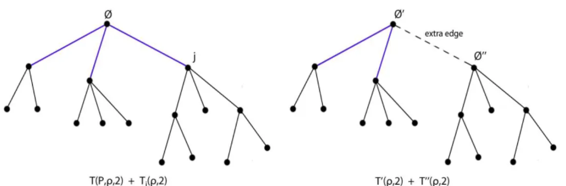
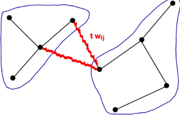
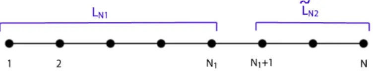
His idea is to break the complete graph GN into two disjoint complete

sub-graphs GN1, GN2 with N1+ N2 and to interpolate between the two situations

(taking into account the normalisation of the parameters) with the aim of proving that the pressure PN is super-additive (or sub-additive).

Finally the Ising model has been recently studied on random graphs.

For example let GN be a diluted Erd¨os-R´enyi graph, namely each pair of

vertices i, j ∈ VN has probability p = (2 c)/(N − 1) to be linked by an

edge and probability 1 − p not to be, independently of the others. Notice the background randomness of the graph structure is added to the specific randomness of the Ising model.

In 2010 Dembo and Montanari computed the thermodynamic limit for the Ising model on such a random graph. Their solution is quite technical but it is based on the fact that the graph GN asymptotically has a locally tree-like

structure. The rest of this chapter is dedicated to the study of their work. In 2011 Contucci, Dommers, Giardin`a and Starr applying an interpolation technique managed to prove that the anti-ferromagnetic spin model (i.e. β < 0) on the diluted Erd¨os-R´enyi graph admits a monotone thermodynamic limit.

1.4

Ferromagnetic spin model on locally

tree-like graphs

Now we’ll study the Ising model on a random graph which locally tends to have no cycles. The whole section is based on the work of Dembo and Montanari and on its generalisations due to Dommers, Giardin`a and Van Der Hofstad.

1.4.1

Definitions concerning the graph structure

Let GN = (VN, EN) , N ∈ N be a sequence of finite random graphs. We

suppose that the vertex set is VN = {1, . . . , N } , while the edge set is random.

That is in general

EN = {ij ∈ P(VN, 2) | εNij = 1}

where ε := (εN

ij)ij, N is a family of random variables taking values 0 or 1 .

value with respect to the randomness of the graph sequence.

As usual on the graph GN the distance between i, j ∈ VN is defined

dN(i, j) = inf{ l ∈ N | ∃ v0, . . . , vl ∈ VN s.t. v0 = i, vl = j, vsvs+1∈ EN} .

For any t ∈ N, denote BN(i, t) the sub-graph of GN induced by the vertices

{j ∈ VN| dN(j, i) ≤ t} .

For any vertex i ∈ VN denote ∂Ni the sets of its neighbours in the graph GN

and denote its degree by

deg_N(i) = |∂Ni| = Card {j ∈ VN| ij ∈ EN} .

As we are interested in the asymptotic behaviour of GN, we give the following

Definition 2. Let P = (Pk)k≥0 be a probability distribution over the

non-negative integers. We say that the graph sequence (GN)N ∈N has asymptotic

degree distribution P if 1 N X i∈VN 1(deg_N(i) = k) −−−→ N →∞ Pk a.s. ∀ k ∈ N .

Now we define an important infinite random graph, the rooted random tree

with independent offspring.

Definition 3. Let P, ρ be two probability distributions over N.

The random independent tree T (P, ρ, ∞) rooted at ∅ is the random tree graph defined recursively as follows.

Let L be a random variable with distribution P and let (Kt,i)t≥1, i≥1 be i.i.d.

random variables with distribution ρ. Let L and (Kt,i)t≥1, i≥1 be independent.

1) Connect the root ∅ to L offspring, which form the 1st _generation

2) Connect each node (t, i) in the tth _{generation to K}

t,i offspring; all

Repeat recursively the step 2) for all t ≥ 1.

We denote T (P, ρ, t) the sub-tree of T (P, ρ, ∞) induced by the first t gene-rations. Notice T (P, ρ, ∞) is locally finite, that is each T (P, ρ, t) is finite. If the distribution P equals ρ, then we’ll denote T (ρ, ∞).

And now come to the definition which characterizes the graphs we will study. Definition 4. We say the random graph sequence (GN)N ∈Nconverges locally

to the random tree T (P, ρ, ∞) if for any t ∈ N and for any T rooted tree with t generations 1 N X i∈VN 1¡BN(i, t) ∼= T ¢ −−−→ N →∞ P ¡ T (P, ρ, t) ∼= T¢a.s.

This definition is slightly different from that given by Dembo and Montanari, we adopt it because some proofs become simpler.

Remark 2. The following statements are equivalent: i. for any T rooted tree with t generations

1 N X i∈VN 1¡BN(i, t) ∼= T ¢ −−−→ N →∞ P ¡ T (P, ρ, t) ∼= T¢a.s.

ii. for any B realisation of the random graph BN(i, t)

1 N X i∈VN 1¡BN(i, t) ∼= B ¢ −−−→ N →∞ P ¡ T (P, ρ, t) ∼= B¢a.s.

iii. for any F invariant by isomorphisms bounded function of a graph 1 N X i∈VN F¡BN(i, t) ¢ −−−→ N →∞ E £ F¡T (P, ρ, t)¢¤a.s.

Proof. iii ⇒ i is obvious.

To prove that ii ⇒ iii, observe that the possible realisations of the random graph GN are only a finite number (since |VN| = N). Therefore we can write

F¡BN(i, t) ¢ =X B F (B) 1¡BN(i, t) ∼= B ¢

where the sum is over all the possible realisations B of BN(i, t) identified by

isomorphisms. Hence by hypothesis ii 1 N X i∈VN F¡BN(i, t) ¢ =X B F (B) 1 N X i∈VN 1¡BN(i, t) ∼= B ¢ _a.s. −−−→ N →∞ X B F (B) P¡T (P, ρ, t) ∼= B¢ = E£F¡T (P, ρ, t)¢¤.

In the end to prove that i ⇒ ii, notice that X

T

P¡T (P, ρ, t) ∼= T¢= 1

where the sum is over all the T rooted tree with t generations, up to isomor-phisms. Hence for any B realisation of BN(i, t) which is not a tree (rooted

with t generations) we have P¡T (P, ρ, t) ∼= B¢ = 0, and on the other side using hypothesis i 1 N X i∈VN 1¡BN(i, t) ∼= B ¢ ≤ 1 −X T 1 N X i∈VN 1¡BN(i, t) ∼= T ¢ _a.s. −−−→ N →∞ 1 −X T P¡T (P, ρ, t) ∼= T¢ = 0 .

Remark 3. If (GN)N ∈N converges locally to T (P, ρ, ∞), then its asymptotic

degree distribution is P . Indeed for all k ∈ N 1 N X i∈VN 1¡deg_N(i) = k¢= 1 N X i∈VN 1¡BN(i, 1) 3 k vertices ¢ −−−→ N →∞ P¡T (P, ρ, 1) 3 k vertices¢= Pk.

Consequently the number of edges |EN| is asymptotically equivalent to NP /2 :

|EN| N = 1 2N X i∈VN deg_N(i) = 1 2N X i∈VN ∞ X k=0 k 1¡deg_N(i) = k¢ −−−→ N →∞ 1 2 ∞ X k=0 k Pk = P 2 .

To end with definitions we specify the proprieties of the distributions P , ρ which will characterize the random tree T (P, ρ, ∞) in the following results.

Let P = (Pk)k≥0 be a probability distribution over the non-negative integers

such that P :=P∞_k=0k Pk< ∞.

Definition 5. We define the size-biased law of P as the probability distri-bution over non-negative integers ρ = (ρk)k≥0 with

ρk = (k + 1) Pk+1 P . Notice that P∞_k=0ρk = 1/P P_∞ k=1k Pk = 1/P P_∞ k=0k Pk= 1 .

Definition 6. Let ² > 0. We say that P has ²-strongly finite mean if:

∞

X

k=n

Pk = O(n−(1+²)) as n → ∞ .

Notice this condition is satisfied if Pk= O(k−(2+²)) as k → ∞.

1.4.2

Definitions concerning the Ising model

From now on fix an inverse temperature β ≥ 0 and a magnetic field B . On a graph G = (V, E) we remind that the Ising model is defined by the following probability measure over all spin configurations σ = (σi)i∈V ∈ {±1}V

µ(σ) = exp ¡ βP_ij∈Eσiσj + P i∈V Biσi ¢ Z(β, B) .

When more clarity is needed, we denote µG this probability measure and

h · i_G the associated expectation.

Notation. When the sequence of graphs (GN)N ∈N is considered, we’ll denote

ZN(β, B), PN(β, B) respectively the partition function and the pressure of

the Ising model on GN. Further we set pN := _N1 PN.

It is useful to consider a subgraph U of G. Given a spin configuration σ ∈

{±1}V _{on the graph G, we denote its restriction to U by σ}

U = (σi| i ∈ U) .

Furthermore we denote µG→U the marginal on U of the measure µG, that is

µG→U(σU) =

X

σG−U

On the other hand µU will simply indicate the measure associated to the

Ising model on the graph U .

We introduce the Ising model on U with positive boundary conditions. That is we define the measure

µ+_U(σ) = 1 Z+ U(β, B) exp¡βX ij∈U σiσj+ X i∈U −∂U Biσi ¢ 1(σi= 1 ∀ i ∈ ∂U)

for all σ spin configuration on U.

As we are going to show, this model is equivalent to the Ising model on U without boundary conditions in the limit of positive infinite magnetic field on ∂U .

Proposition 7. Let U be a subgraph of the graph G. Then in the limit

Bi ≡ B → ∞ for all i ∈ ∂U we have

i. µU(σ) −→ µ+U(σ) for all σ spin configuration on U ;

ii. µG(σ) −→ µ+U(σU) · eµG−U(σG−U) for all σ spin configuration on G ,

where eµG−U is the measure associated to the Ising model on G−U with

mag-netic field increased on ∂(G−U), precisely

e

Bi =

(

Bi+ β if i ∈ ∂(G−U)

Bi if i ∈ (G−U) − ∂(G−U)

Proof. i. Fix a spin configuration σ on the graph U.

Suppose that ∂U) contains n vertices, on which there are p ≥ 0 spin variables

σi with value −1 and n − p with value 1.

Write the probability of σ in the Ising model on U with no boundary condi-tions, isolating the effect of the external field on the boundary:

µU(σ) = exp¡βP_ij∈Uσiσj+ P i∈UBiσi ¢ P τexp ¡ βP_ij∈Uτiτj+ P i∈UBiτi ¢ = = exp ¡ βP_ij∈Uσiσj + P i∈U −∂UBiσi ¢ e−pB _e(n−p)B P_n q=0 P τ ∈Cqexp ¡ βP_ij∈Uσiσj + P i∈U −∂UBiσi ¢ e−qB _e(n−q)B

where Cq is the set of spin configurations τ on U such that on ∂U there are

q spin variables τi taking value −1 and n − q taking value 1.

Observe that e−pB_e(n−p)B e−qB_e(n−q)B = _e2(p−q)B1 and e2(p−q)B _−−−→ B→∞        0 if q > p 1 if q = p ∞ if q < p . Therefore if p = 0 µU(σ) −−−→ B→∞ exp¡βP_ij∈U σiσj+ P i∈U −∂UBiσi ¢ P τ ∈C0exp ¡ βP_ij∈Uσiσj+ P i∈U −∂UBiσi ¢ , whereas if p ≥ 1 µU(σ) −−−→ B→∞ 0 .

Hence in both cases it is limB→∞µU(σ) = µ+_U(σ) .

ii. Now let σ be a spin configuration on the graph G. Observe that by definition of ∂U, one can divide the following disjoint cases:

ij ∈ G ⇔ (ij ∈ U) xor (ij ∈ G−U) xor (ij ∈ G, i ∈ ∂U, j ∈ ∂(G−U)) ; i ∈ G ⇔ (i ∈ U) xor (i ∈ G − U) .

Therefore the probability of σ can be split in

µG(σ) = C exp ¡ βX ij∈U σiσj + X i∈U Biσi ¢ · · exp¡β X ij∈G−U σiσj + X i∈G−U Biσi ¢ · exp¡β X ij∈G i∈∂U, j∈∂(G−U ) σiσj ¢

The first term up to a constant equals µU(σU), therefore as proven in i. it

converges to µ+_U(σU) as B → ∞.

Since µ+_U(σU) contains 1(σ∂U ≡ 1), as B → ∞ the third term can be

substi-tuted by exp¡ P_{j∈∂(G−U )}β σj

¢ .

The second term multiplied by this new term equals eµG−U(σG−U) with

mag-netic field increased of β on ∂(G−U).

1.4.3

Results on the trees: the root magnetisation

In this subsection we’ll see some preliminary results about the Ising model on a tree (deterministic or random). These results concern in particular the magnetisation of the root. Indeed this will turn out to be the fundamental quantity to study in order to compute the thermodynamic limit on a sequence of graphs locally convergent to a tree.

Let start with a simple but important lemma which permits to restrict the Ising model on a tree to any sub-tree without difficulties.

Lemma 8. Let T be a finite tree. Let U be a sub-tree of T .

For every i ∈ ∂U, let Ti be the maximal sub-tree of T − U + i rooted at i.

The marginal on U of the measure associated to the Ising model on T is the measure associated to an Ising model on U, with magnetic field increased on the boundary. Precisely:

µT →U = eµU with eBi =

(

atanhhσii_Ti ≥ Bi if i ∈ ∂U

Bi if i ∈ U − ∂U

.

Figure 1.2: The tree T and its sub-tree U . Each vertex i ∈ ∂U is the root of a

maximal sub-tree Ti of T − U + i.

Proof. Denote W := T − U, the complementary forest of U in T .

Notice that the union of the trees Ti, i ∈ ∂U is equal to W + ∂U, since the

Ti’s are maximal. Furthermore observe that for any i, j ∈ ∂U, i 6= j the trees

Now for any σU spin configuration on U µT →U(σU) def= X σW µT(σU, σW) = 1 ZT X σW exp¡βX ij∈T σiσj + X i∈T Biσi ¢ = 1 ZT exp¡βX ij∈U σiσj + X i∈U −∂U Biσi ¢ X σW exp¡β X ij∈W +∂U σiσj + X i∈W +∂U Biσi ¢ ,

but since W is the disjoint union of the Ti− i ’s with i ∈ ∂U

X σW exp¡β X ij∈W +∂U σiσj + X i∈W +∂U Biσi ¢ = Y i∈∂U X σ_Ti−i exp¡β X hk∈Ti σhσk+ X h∈Ti Bhσh ¢ = Y i∈∂U X σ_Ti−i ZTi µTi(σTi) = Y i∈∂U ZTi µTi→i(σi) , hence it follows µT →U(σU) = C exp ¡ βX ij∈U σiσj+ X i∈U −∂U Biσi ¢ Y i∈∂U µTi→i(σi) .

Compute µTi→i(σi). For any random variable X taking values ±1 it’s easy

to check that

P[X = ±1] = 1 ± E[X] 2 , further observe that for any −1 ≤ α ≤ 1

1 ± α (1 − α2₎1/2 = ¡ 1 + α 1 − α ¢_±1/2 = exp(± atanh α) , therefore in our case:

µTi→i(σi) = 1 + σihσii_Ti 2 = (1 − hσii2_Ti)1/2 2 exp ¡ σi atanhhσii_Ti ¢ .

Substitute in the previous expression of µT →U(σU) and find

µT →U(σU) = C exp ¡ βX ij∈U σiσj + X i∈U −∂U Biσi+ X i∈∂U e Biσi ¢ ,

with eBi = atanhhσii_Ti for any i ∈ ∂U .

To conclude the proof it remains only to check that atanhhσii_Ti ≥ Bi for any

i ∈ ∂U . To do it use the G.K.S. inequality: hσii_Ti ≥ hσii_{i} = P σi=±1σie Biσi P σi=±1e Biσi = eBi− e−Bi eBi + e−Bi = tanh Bi.

Notation. Given a rooted tree T (t) of t generations we denote Bd T (t) the set of vertices composing its tth _generation.

Lemma 9. Let T (1) be a finite tree rooted at ∅ and with only one generation.

The magnetisation of the root in the Ising model on T (1) is: hσ∅i_{T (1)} = tanh £ B∅+ X i son of ∅ atanh(tanh β tanh Bi) ¤ . Proof. For brevity denote T = T (1).

As T is a rooted tree with only one generation, T = ∅ + Bd T and the only edges are those which link ∅ to its offspring.

With these remarks write hσ∅i_T developing the sums over σ∅ = ±1:

hσ∅i_T = X σ∈{±1}T σ∅µT(σ∅) = X σ∈{±1}Bd T £ exp¡ X i∈Bd T β σi+ X i∈Bd T Biσi+ B∅ ¢ − exp¡−X i∈Bd T β σi+ X i∈Bd T Biσi− B∅ ¢¤ X σ∈{±1}Bd T £ exp¡ X i∈Bd T β σi+ X i∈Bd T Biσi+ B∅ ¢ + exp¡−X i∈Bd T β σi+ X i∈Bd T Biσi− B∅ ¢¤

Now that all interactions are made explicit, it’s simple to rewrite each term: X σ∈{±1}Bd T exp¡±X i∈Bd T β σi+ X i∈Bd T Biσi± B∅ ¢ = e±B∅ X σ∈{±1}Bd T Y i∈Bd T e(±β+Bi) σi = e±B∅ Y i∈Bd T X σi=±1 e(±β+Bi) σi _{= e}±B∅ Y i∈Bd T ¡ e±β+Bi_{+ e}−(±β+Bi)¢

hence, substituting in the previous equality,

hσ∅i_T = eB∅Q i∈Bd T ¡ eβ+Bi + e−β−Bi¢− e−B∅Q i∈Bd T ¡ e−β+Bi + eβ−Bi¢ eB∅Q i∈Bd T ¡ eβ+Bi+ e−β−Bi¢+ e−B∅Q i∈Bd T ¡ e−β+Bi + eβ−Bi¢ .

To conclude it’s only matter of rewriting more compactly this equation. Start from here and use two times the fact that α = x−y_x+y ⇔ 1+α

1−α = xy to compute: 1 + hσ∅iT 1 − hσ∅i_T = e2B∅ Y i∈Bd T eβ+Bi+ e−β−Bi e−β+Bi + eβ−Bi = e 2B∅ Y i∈Bd T 1 + tanh β tanh Bi 1 − tanh β tanh Bi

Therefore: atanhhσ∅iT = 1 2 log 1 + hσ∅i_T 1 − hσ∅iT = B∅+ X i∈Bd T 1 2 log 1 + tanh β tanh Bi 1 − tanh β tanh Bi = = B∅+ X i∈Bd T atanh(tanh β tanh Bi) .

Notation. Consider the Ising model on a finite rooted tree T (t) composed of

t generations, with magnetic field on its nodes B = (Bi)i∈T (t) and the inverse

temperature β. As usual the expected value w.r.t. the spin variables in this model is denoted

h · i_{T (t)}

Now consider the Ising model with magnetic filed increased only on Bd T (t) by a vector H = (Hi)i∈Bd T (t). We denote the expected value w.r.t. the spin

variables in this new model by

h · i_{T (t), +H}

The following lemma is a direct consequence of lemmas 8 and 9. This state-ment will be used often, so it’s opportune to write it explicitly.

Lemma 10. Let T (t +1) be a finite tree rooted in ∅ and composed of t +1

generations. Let T (t) be its sub-tree induced by the first t generations. The magnetisation of the root in the Ising model on T (t +1) equals the mag-netisation of the root in the Ising model on T (t) with increased magnetic field on Bd T (t). Precisely:

hσ∅i_{T (t+1)} = hσ∅i_{T (t), +H} with Hi =

X

j son of i

ξβ(Bj) ∀ i ∈ Bd T (t)

where we set ξβ(x) := atanh(tanh β tanh x) .

Proof. Apply lemma 8 choosing T = T (t +1) and U = T (t) 3 ∅: hσ∅iT (t+1) = hσ∅iT (t)| Bi → eBi ∀ i ∈ ∂T (t)

where for any i ∈ ∂ T (t) eBi = atanhhσiiTi(1) and Ti(1) is the maximal

sub-tree rooted in i and contained in T (t +1) − T (t) + i. Notice Ti(1) is the sub-tree induced by i and its offspring.

Therefore by lemma 9, compute for any i ∈ ∂ T (t) e

Bi = atanhhσii_Ti = Bi +

X

j son of i

ξβ(Bj) .

To conclude observe that

Bd T (t) = ∂ T (t) t {i ∈ tthgeneration of T (t) | i has no sons} hence there is no problem to write

hσ∅iT (t+1) = hσ∅iT (t)| Bi → Bi +

X

j son of i

ξβ(Bj) ∀ i ∈ Bd T (t) .

Now we are ready to write a recursive formula for the root magnetisation, a central result for the next investigations on random graphs.

Proposition 11. Let T (t) be a finite tree with root in ∅ and composed of t

generations.

The atanh of the magnetisation of the root in the Ising model on T (t) is:

atanhhσ∅i_{T (t)} = B∅+ X i1son of ∅ ξβ µ Bi1+ X i2son of i1 ξβ ¡ . . . Bit−1+ X itson of it−1 ξβ(Bit) ¢¶

where the function ξβ is defined by

Proof. Proceed by induction on the number t ∈ N of generations of the tree.

For t = 0 it’s simply T (0) = {∅} , then

hσ∅iT (0) = P σ∅=±1σ∅ e B∅σ∅ P σ∅=±1e B∅σ∅ = eB∅− e−B∅ eB∅+ e−B∅ = tanh B∅.

Now assume the result is true for a t ≥ 0 and prove it for t + 1.

Consider T (t), the sub-tree of T (t +1) composed by the first t generations. By lemma 10

hσ∅i_{T (t+1)} = hσ∅i_{T (t), +H}

where for all it∈ Bd T (t) Hit =

P

it+1son of itξβ(Bit+1) .

On the other hand by inductive hypothesis atanh hσ∅iT (t), +H = B∅ + X i1son of ∅ ξβ µ Bi1 + X i2son of i1 ξβ ¡ . . . Bit−1 + X itson of it−1 ξβ(Bit + Hit) ¢¶

Substitute in this expression the expression of Hit and the thesis is proved

for t + 1.

The form of proposition 11 simplifies if we consider uniform magnetic field

B and a random tree T (ρ, t) defined as in subsection 1.4.1.

Corollary 12. Let (Kt, i)t≥0, i≥1 be i.i.d. integer r.v. with distribution ρ such

that a.s. 0 ≤ Kt, i< ∞ .

Let T (ρ, ∞) be a random tree rooted in ∅ and such that the offspring size of the ith _{vertex of the t}th _{generation (root included) is K}

t, i.

Suppose the inverse temperature is 0 ≤ β < ∞ and the external field is uniformly Bi ≡ B ∈ R . And set for any t ∈ N

h(t) _{:= atanhhσ}

∅i_{T (ρ, t)}

The probability distribution of the magnetisation of the root ∅ in the Ising model on the tree T (ρ, t) is such that

(

h(t+1) d_{= B +}PK

i=1ξβ(h(t)i ) ∀ t ∈ N

where:

• ξβ(x) = atanh(tanh β tanh x)

• (h(t)_i )i≥1 are i.i.d. r.v. with the distribution of h(t)

• K is a r.v. of distribution ρ, independent of (h(t)_i )i≥1, t≥0.

Proof. Remind the definition h(t) _{:= atanhhσ}

∅i_{T (ρ, t)}, apply the proposition

11 and use the independence of the numbers of offspring:

h(0) = B , h(1) _{= B +} K0 X i1=1 ξβ(B)= B +d K X i=1 ξβ(h(0)) , h(2) _{= B +} K0 X i1=1 ξβ ¡ B + K_{X1, i1} i2=1 ξβ(B) | {z } d = h(1) ¢ _d = B + K X i=1 ξβ(h(1)) , h(3) = B + K0 X i1=1 ξβ µ B + K_{X1, i1} i2=1 ξβ ¡ B + K_{X2, i2} i3=1 ξβ(B) | {z } d = h(2) ¢¶ _d = B + K X i=1 ξβ(h(2)) , . . . etcetera.

The previous corollary gives a distributional recurrence for the the root mag-netisation of a random tree T (ρ, t) . We are interested its behaviour when

t → ∞ and we expect to obtain a fixed point of the recurrence.

Using the Ising model with positive boundary conditions, we will be able to prove that there exists a unique positive fixed point.

Notation. Given a rooted tree T (t) of t generations denote h · i+_{T (t)} the ex-pected value w.r.t. the Ising model on T (t) with positive conditions on Bd T (t) .

Proposition 13. Let T (t) be a finite tree rooted in ∅ and composed of t

generations. Suppose the external field is B = (Bi)i, Bi ≥ Bmin > 0 and the

inverse temperature is 0 ≤ β ≤ βmax < ∞.

The effect of positive boundary conditions on the magnetisation of the root in the Ising model on T (t) vanishes when t grows. Precisely:

0 ≤ hσ∅i+_{T (t)}− hσ∅i_{T (t)} ≤

M t , with M = M(Bmin, βmax) = sup0<x≤βmaxx/

¡

atanh(tanh x tanh Bmin)

¢

< ∞ . Proof. For any s ≤ t denote T (s) the sub-tree of T (t) induced by the first s

generations. Then, given an additional magnetic field H on Bd T (s), denote

h·i_{T (s), +H} the expectation w.r.t. the Ising model on the tree T (s) with the magnetic field B increased by H only on Bd T (s).

The first inequality is a direct consequence of G.K.S.:

hσ∅iT (t)+ = hσ∅iT (t), +∞ ≥ hσ∅iT (t).

To deal with the second inequality begin observing that the case β = 0 is trivial, since the root does not interact with the boundary. Formally:

hσ∅i_{T (t)} = P σσ∅ exp ¡ P i∈T (t)Biσi ¢ P σexp ¡ P i∈T (t)Biσi ¢ = P σ∅σ∅ e B∅σ∅P σ0exp ¡ P i6=∅Biσi ¢ P σ∅e B∅σ∅P σ0exp ¡ P i6=∅Biσi ¢ = = e B∅− e−B∅ eB∅+ e−B∅ = tanh B∅,

where here σ0 _{denotes the vector σ minus its component σ}

∅; and similarly

one finds that also hσ∅i+_{T (t)}= tanh B∅.

Now assume β > 0 and fix s = 1, . . . , t .

I) Start studying the positive boundary conditions case. Use the lemma 10 :

hσ∅i+T (s)= hσ∅iT (s), +∞= hσ∅iT (s−1),+ H

where for every i ∈ Bd T (s −1)

Hi =

X

j son of i

and ∆i denotes the number of sons of the node i. Hence, setting ∆ = (∆i)i,

hσ∅i+_{T (s)} = hσ∅i_{T (s−1), +β ∆} (1.4)

And by G.K.S. it follows that s 7→ hσ∅i+_{T (s)} is monotonically decreasing:

hσ∅i+T (s)= hσ∅iT (s−1), +β ∆ ≤ hσ∅iT (s−1), +∞ = hσ∅i+T (s−1).

II) Now study the free boundary conditions case. Use the G.K.S. inequality and the lemma 10 :

hσ∅i_{T (s)} ≥ hσ∅i_{T (s), +Bmin−B} = hσ∅i_{T (s−1), +H}0

where for all i ∈ Bd T (s −1)

H0 i =

X

j son of i

atanh(tanh β tanh Bmin) = ξβ(Bmin) ∆i

Hence, setting ξ0

β := ξβ(Bmin) > 0 ,

hσ∅iT (s) ≥ hσ∅iT (s−1), +ξ0

β∆ (1.5)

And by G.K.S. it follows that s 7→ hσ∅i_{T (s)} is monotonically increasing:

hσ∅i_{T (s)} ≥ hσ∅i_{T (s−1), +ξ}0

β∆ ≥ hσ∅iT (s−1) .

III) By the G.H.S. inequality, the function h 7→ hσ∅iT (s−1), +h ∆ =: f (h) is

concave. Hence, since ξ0

β = atanh(tanh β tanh Bmin) < β, it follows that

f (β) − f (0) β − 0 ≤ f (ξ0 β) − f (0) ξ0 β − 0

Rewriting this condition one obtains

hσ∅i_{T (s−1), +β ∆}− hσ∅i_{T (s−1)} ≤ M ¡ hσ∅i_{T (s−1), +ξ}0 β∆− hσ∅iT (s−1) ¢ (1.6) with M := sup{x/ atanh(tanh x tanh Bmin) | 0 < x ≤ βmax}, which is finite

Now bound the effect of positive boundary conditions on the root magneti-sation in the model on T (s), using equations (1.4), (1.5), (1.6)

hσ∅i+_{T (s)}− hσ∅i_{T (s)} ≤ hσ∅i_{T (s−1), +β ∆}− hσ∅i_{T (s−1)} ≤ M¡hσ∅iT (s−1), +ξ0 β∆− hσ∅iT (s−1) ¢ ≤ M¡hσ∅iT (s)− hσ∅iT (s−1) ¢ .

Then use the different monotonicity of s 7→ hσ∅i+_{T (s)} and s 7→ hσ∅i_{T (s)} to

conclude: t¡hσ∅i+T (t)− hσ∅iT (t) ¢ ≤ t X s=1 ¡ hσ∅i+T (s)− hσ∅iT (s) ¢ ≤ M t X s=1 ¡ hσ∅iT (s)− hσ∅iT (s−1) ¢ = M¡hσ∅iT (t)− hσ∅iT (0) ¢ ≤ M .

Using corollary 12 and proposition 13 we can prove the following probability result, which characterizes the root magnetisation on the random tree T (ρ, t) as t → ∞.

Proposition 14. Let B > 0 , 0 ≤ β < ∞ and let ρ be a probability

distribu-tion over N.

Consider a sequence (h(t)₎

t∈N of r.v.’s whose distributions are defined by the

recursive relation (1.3), that is

( h(t+1) d_{= B +}PK i=1ξβ(h (t) i ) ∀ t ∈ N h(0) _{= B} where • ξβ(x) = atanh(tanh β tanh x)

• (h(t)_i )i≥1 are i.i.d. r.v. with the same distribution of h(t)

• K is a r.v. of distribution ρ, independent of (h(t)_i )i≥1, t≥0 .

i. (h(t)₎

t∈N is stochastically monotone (that is it admits a coupling which

is monotone a.s.)

ii. there exists a r.v. h∗ _{such that h}(t) _−−−→d

t→∞ h

∗

iii. h∗ _{is the only (in distribution) r.v. supported on [0, ∞[ such that}

h∗ d_{= B +} K X i=1 ξβ(h∗i) (1.7) with (h∗

i)i≥1 i.i.d., distributed as h∗, independent of K.

Proof. I) Consider the random rooted tree T (ρ, ∞) and the Ising model on

it with inverse temperature β and magnetic field B. By corollary 12 a coupling of (h(t)₎

t∈N is given by

h(t) := atanhhσ∅i_{T (ρ, t)} ∀ t ∈ N .

As seen in the proof of proposition 13 (or simply by G.K.S. inequality), the sequence t 7→ hσ∅i_{T (ρ, t)} is monotonically increasing. Hence also t 7→ h(t) is

monotonically increasing. Therefore there exists h∗ _{≥ B such that}

h(t) _−−−→

t→∞ h

∗ _a.s.

and so also in distribution. Then, by definition, for any φ : R+ → R

conti-nuous and bounded E[φ(h∗_{)] = lim} t→∞E[φ(h (t)_{)] = lim} t→∞E £ φ¡B + K X i=1 ξβ(h(t−1)i ) ¢¤ Now since h(t−1)_i −−→ hd ∗ i as t → ∞ and ¡ (h(t−1)_i )i, K ¢

are independent as well as ¡(h∗

i)i, K

¢

, it is also true that ¡(h(t−1)_i )i, K

¢ _d

−−→ ¡(h∗ i)i, K

¢

as t → ∞ (this can be easily proven via the characteristic functions). Therefore by dominated convergence lim t→∞E £ φ¡B + K X i=1 ξβ(h(t−1)i ) ¢¤ = E£φ¡B + K X i=1 ξβ(h∗i) ¢¤ .

Hence E[φ(h∗_{)] = E}£_φ¡_{B +}PK

i=1ξβ(h∗i)

¢¤

, and by arbitrariness of φ conti-nuous and bounded conclude that

h∗ d= B +

K

X

i=1

ξβ(h∗i) .

II) It remains to prove that h∗ _{< ∞ and that any other r.v. supported on}

[0, ∞[ and satisfying the same fixed point distributional equation is neces-sarily equal in distribution to h∗_{. Define}

h(t), + := atanhhσ∅i+T (ρ, t) ∀ t ∈ N .

Since the model with positive boundary conditions is equivalent to that one with no boundary conditions when the magnetic field on Bd T (ρ, t) goes to infinity, ₍

h(t+1), + d_{= B +}PK

i=1ξβ(h(t),+i ) ∀ t ∈ N

h(0), + _{= ∞} (1.8)

where (h(t), +_i )i are i.i.d. copies of h(t), + and they’re independent of K.

As seen in the proof of proposition 13, the sequence t 7→ hσ∅i+_{T (ρ, t)} is

mono-tonically decreasing. Hence also t 7→ h(t), + _{is monotonically decreasing and}

so there exists h∗, +_{< ∞ (notice h}(1), +_{< ∞) such that}

h(t), + −−−→

t→∞ h

∗, + _a.s.

Proceeding as before one proves that

h∗, + d_{= B +} K

X

i=1

ξβ(h∗, +i )

with (h∗, +_i )i i.i.d. copies of h∗, +, independent of K.

Now let h∗∗ _{be a r.v. supported on [0, ∞] and verifying the same fixed point}

distributional equation 1.7. Without loss of generality assume it is defined on the same probability space as T (ρ, ∞).

Notice that, since ξβ ≥ 0 on [0, ∞], necessarily h∗∗≥ B. Therefore

Now take i.i.d. copies of each of these three r.v.’s, independent of K and coupled so they still verify the previous order relation. Then apply the func-tion B +PK_i=1ξβ(·) and, since it is a monotonically increasing function w.r.t.

each variable, one gets h(1) _{≤ h}∗∗_{≤ h}(1), +_.

Repeat this procedure t times and then let t → ∞ :

h(t) ≤ h∗∗≤ h(t), + ∀ t ∈ N ⇒ h∗ ≤ h∗∗≤ h∗, + a.s.

But on the other hand by proposition 13

| tanh(h(t), +_{) − tanh(h}(t)_{)| = |hσ}

∅i+_{T (ρ, t)}− hσ∅i_{T (ρ, t)}| ≤

M

t −−−→t→∞ 0

therefore tanh h∗, +_{= tanh h}∗ _{⇒ h}∗, + _{= h}∗_{. Thus conclude}

h∗ _{= h}∗∗_{= h}∗, + _{∈ [B, ∞[ a.s.}

and so also in distribution.

We conclude this subsection about trees proving that the root magnetisation is Lipschitz continuous w.r.t. β uniformly in number of generations t, so that the Lipschitz continuity is preserved in the limit t → ∞ .

Notation. Consider the Ising model on a finite rooted tree T (t) composed of t generations, with magnetic field B and inverse temperature β .

To make explicit the parameters, we’ll use the following notation for the magnetisation of the root ∅:

mt(β, B) := hσ∅i_{T (t)}.

Proposition 15. Let T (t) be a finite rooted tree rooted with t generations.

Suppose the external field is fixed B = (Bi)i, Bi ≥ Bmin > 0, while the

inverse temperature can be 0 < βmin ≤ β1 ≤ β2 < ∞.

The magnetisation of the root in the Ising model is Lipschitz continuous w.r.t. β, uniformly in t. Precisely:

0 ≤ mt(β2, B) − mt(β1, B) ≤ C (β2 − β1) ,

with C = C(βmin, Bmin) = supβmin≤x<∞1/

¡

atanh(tanh x tanh(Bmin)

¢