Ionospheric Plasma Response to the Anomalous Minimum of the Solar Cycle 23/24: Modeling and Comparison with IRI-2012

(1)

Alma Mater Studiorum - Universit`

a di Bologna

DOTTORATO DI RICERCA IN

GEOFISICA

Ciclo XXIX

Settore Concorsuale di afferenza: 04/A4

Settore Scientifico Disciplinare: GEO/10

Ionospheric plasma response to the anomalous

minimum of the solar cycle 23/24: modeling and

comparison with IRI-2012

Presentata da: Luigi Perna

Coordinatore Dottorato:

Prof. Nadia Pinardi

Supervisore:

Prof. Michele Dragoni

Relatore:

Dr. Michael Pezzopane (INGV)

(2)

A chi è l’amore, a chi è il sacrificio, a chi è la pazienza, a chi è la passione, a chi è il sostegno, a chi è il sorriso. ii

(3)

Introduction

The section of the terrestrial atmosphere included between the thermopause (∼500 km) and the stratopause (∼50 km) is identified with the term ionosphere. The ionosphere represents the portion of the Earth’s atmosphere where the density of free electrons is high enough to influence the propagation of radio waves.

The first hypothesis about the existence of a conducting atmospheric layer was formulated at the beginning of the XIX century, when Carl Gauss and Balfour Stewart hypothesized the existence of atmospheric electric currents to explain the observed variations of the Geomagnetic Field (GF). The clear proof of the ionosphere existence was given on 12 December 1901, when Guglielmo Marconi established a radio link between the cities of Poldhu (UK) and St. John’s (Canada).

The ionosphere can be considered a minority plasma, meaning that the ionized component (ions and free electrons) represents a smaller fraction than the neutral one. The GF interacts with the ionospheric plasma, therefore they talk about a magnetoionic plasma or simply a magnetoplasma. The study of the electromagnetic waves propagation through a magnetoplasma represents the magnetoionic theory, which became of great interest since the beginning of the XX century.

The observed pattern of the ionosphere is produced by the differential interaction between the neutral atmospheric species and the ionizing solar radiation, which produces a vertical electron density profile characterized by several relative maxima and minima. At every max-imum, a specific frequency, called critical frequency, and an ionospheric layer are associated. The critical frequencies of the ionospheric layers are very important, representing the maximum frequencies at which a radio wave sent vertically towards the ionosphere is reflected towards the Earth. The absolute electronic density maximum (NmF2) of the vertical profile is associated to the diurnal F2 layer (or the nighttime F region) and the correspondent critical frequency is called foF2. This is the most important ionospheric parameter, because it represents the maximum frequency vertically reflected by the ionosphere.

Besides considering foF2, the ionospheric plasma is investigated by analyzing NmF2 and the corresponding height hmF2. foF2 is strictly linked to NmF2, by virtue of the plasma frequency

formula: 𝑁 𝑚F2[m−3] = 1.24 · 1010(𝑓 𝑜F2[MHz])2.

The climatological pattern of the aforementioned ionospheric parameters is strongly influ-enced by the latitude, longitude, geomagnetic activity and solar activity. However, the solar activity represents the most relevant cause of the ionospheric variability.

During the last decades, the interest in studying the ionosphere has strongly increased because: (1) the ionosphere swiftly reacts to variations of the Sun-Earth environment and it is then expected to be strictly linked to the Sun activity; (2) long- and short-time variations of the ionosphere significantly affect the communications Earth-Earth, Earth-satellite and satellite-satellite; (3) possible signatures of the greenhouse gases increase could be observed in the ionospheric parameters long-term trends.

(6)

Introduction

The last solar minimum, between the solar cycle 23 and 24 (minimum 23/24), has shown unprecedented characteristics, being the longest and quietest period since the advent of space-based measurements. The minimum interested the years between 2007 and 2010, with 2008 and 2009 representing the deepest phase for which a very low solar activity occurred. For the minimum 21/22, 176 spotless days were registered for the two years 1986-1987; for the minimum 22/23 (years 1996-1997), the observed spotless days were 226; for the years 2008-2009 of the last minimum, 527 days without sunspots have been registered, revealing an extremely quiet solar activity period. In addition, the last solar minimum has been characterized by an uncommon long duration. As a first step, the beginning of the minimum has been set around March 2006 and many predictions of the start and length of solar cycle 24 were given thereafter. In 2007, the solar cycle 24 Prediction Panel anticipated that the solar minimum marking the onset of cycle 24 would occur in March 2008 (±6 months), but the date was then corrected to August 2008 and later to December 2008. Actually, the minimum was registered in the middle of 2009 and thus more than 2 years after the earliest prediction and with a whole 23 cycle length of 12 years and 6 months, that is 18 months longer than the “canonical” 11-year solar cycle.

The unique features that characterized the last minimum have been confirmed by numerous observations: (1) the magnetic field at solar poles was approximately 40% weaker than that of cycle 22/23; (2) a 20% drop in solar-wind pressure has been measured since the mid-1990s, touching the lowest point since the start of measurements in the 1960s; (3) solar-wind speed and radiation-belt flux were lower than those of previous minima; (4) the thermospheric densities at an altitude of 400 km were the lowest observed in the 43-year (1967-2010) database, and were anomalously lower, by 10-30%, than the climatologically expected levels; (5) for the latter half

of 2008, the O+_/H+ _{transition height, that represents a sensitive indicator of both the solar}

extreme ultra violet ionizing flux and the dynamics of the topside ionosphere, was much cooler and much closer to the planet than expected.

Because of the strong influence that ionospheric disturbances can have in particular in radio communications, there is an increasing interest in studying the ionospheric plasma response to extreme solar activity conditions, and the corresponding possible consequences on the near-Earth environment. Under the aforementioned unprecedented conditions, the minimum of the solar cycle 23/24 provides a perfect natural window to study the ionospheric plasma response under a very low and prolonged solar activity.

The main ionospheric ionization source is the radiation in the Ultra Violet band (120-400 nm) and in particular in the Extreme Ultra Violet band (EUV, 0.1-120 nm). The solar EUV irradiance explains around 90% of the variance of ionospheric parameters such as foF2 and hmF2, and solar indices which refer to wavelengths in the EUV band are theoretically the most appropriate to describe the ionospheric variability. Nevertheless, accurate measurements of EUV/UV irradiance are possible only from above the terrestrial atmosphere. Consequently, EUV continuous measurements started only with the launch of the Solar Heliospheric Obser-vatory (SOHO), in the mid-1990s. Moreover, instruments used to perform measurements in these bands quickly degrade because of the intense UV and EUV exposure, and monitoring of this instrumental degradation is particularly difficult. Therefore, continuous and reliable EUV datasets are not common and, for ionospheric studies, it is necessary to use solar indices with longer datasets that can be considered good proxies for the solar activity in these wavelengths.

Among the numerous available indices, the solar radio flux at 10.7 cm, namely 𝐹10.7,

repre-sents the most widely used solar activity proxy, being used by ionospheric and thermospheric models such as the IRI (International Reference Ionosphere) model and the NRLMSISE-00 model. The solar radiation at 10.7 cm can be easily measured with ground-based instruments,

(7)

Introduction

and this is why 𝐹10.7 has a long and continuous dataset starting since 1947. Nevertheless, the

reliability of this index as a good proxy for both the general solar activity and the radiation in the EUV band has been questioned during the last solar minimum. It has been shown that the decrease of the solar EUV irradiance from the minimum 22/23 to the last minimum was much

larger (15%) than the decrease of 𝐹10.7 (5%). Furthermore, marked changes in the long-term

relation between the EUV irradiance and 𝐹10.7 have been observed since 2006, with EUV levels

decreasing more than those of 𝐹10.7. Therefore, it has been highlighted how 𝐹10.7 can no more

be considered both a good EUV proxy and a good solar activity proxy for ionospheric purposes. In light of the very particular conditions observed for the last solar minimum and of the

variations in the relation between the EUV radiation and the index 𝐹10.7, a deeper analysis of

the relations between parameters that characterize the ionospheric plasma and the most widely used solar indices is of primary importance. Focusing the attention on the main ionospheric parameter foF2, which shows a marked dependence on solar activity variations, it is worth noting that the analysis of relationships (foF2 vs Solar Index ) results to be essential because: (1) every ionospheric model is based on these relations; (2) when accurate, these relations can be used to “clean” ionospheric time series from the solar activity influence, in order to extract possible ionospheric signatures of the greenhouse effect.

As mentioned before, the solar activity represents the main cause of the observed ionospheric variability. Therefore, the knowledge of relations that link foF2 with solar activity indices is essential to improve the performances of ionospheric models.

Over the last four decades, long-term prediction models of the ionospheric conditions have represented an important tool for both applied science and theoretical studies. The systematic collection of regular observations and the evolution of computing systems allowed William B. Jones and Roger M. Gallet to produce, in 1965, the first global model for long-term mapping of foF2 and the propagation factor for a distance of 3000 km, namely M (3000)F2.

In the last years, together with a long-term description of the ionospheric characteristics, the interest has increased in a short-term forecasting and nowcasting of the ionosphere. With the aim of short-time forecasting and nowcasting on a continental scale, numerous international projects have been developed, such as the COST (Cooperation in Science and Technology)

actions, the European projects DIAS (DIgital upper Atmosphere Server ; http://www.iono.noa.

gr/DIAS/)and ESPAS (Near-Earth Data Infrastructure for e-Science; http://www.espas-fp7.

eu/); also working programs has been opened, such as IPS (Ionospheric Prediction Service,

Australia) and NOAA (National Oceanic and Atmospheric Administration, USA).

Recent advances in global and regional networks of real-time ionosondes and ground-based dual-frequency GNSS (Global Navigation Satellite System) receivers, together with data-driven ionospheric modeling, have brought new insights to ionospheric physics, with significant impro-vements of prediction and forecasting modeling.

A clear proof of this is the possibility to obtain from satellite “top-side” electron density profiles (above the electron density peak), which is not possible from ground-based ionosondes. HF (High Frequency) radio communications are widely used in many fields like: emergency services, strategic implementations, in-flight information and communications, and general ra-dio services. As mentioned before, the ionosphere represents the portion of the atmosphere that significantly influences the HF propagation. For example, disturbed conditions of the solar-terrestrial environment (such as those caused by geomagnetic storms) may seriously affect the trans-ionospheric transmissions used by navigational systems. Therefore, the ionospheric modeling, that can be global or regional/local, represents a primary goal.

Global ionospheric models usually use ground-based and in-situ data to provide empirically

(8)

Introduction

a global mean description of the ionospheric parameters. Nevertheless, when an accurate and quick description of the ionospheric features for a limited sector is needed, regional/local models are preferable. The limit cases of regional/local models are the Single-Station Models (SSMs) that use data only from one station, providing a very accurate and simple description of the ionosphere around the corresponding site.

Nowadays, the most widely used global ionospheric model is the IRI model that represents the reference model for the ionospheric community. The IRI is an international project spon-sored by the Committee on Space Research (COSPAR) and the International Union of Radio Science (URSI), based on an extensive database, and able to capture much of the repeatable characteristics of the ionosphere for quiet and storm-time periods, such as the electron density, the electron content, the plasma temperatures and the ion composition, as a function of height, location, and local time.

The Simplified Ionospheric Regional Model (SIRM ) is a European regional model based on data from seven ionosondes. The model has been developed in the early 90s and provides an accurate description of the monthly median values of several ionospheric characteristics. SIRM is a very simple model that takes into account the dependence of the parameters from the solar activity, by means of linear regressions, and uses a Fourier analysis to characterize and forecast the variations of the ionospheric characteristics. Due to the longitudinally limited

sector considered (40∘), the model takes into account only latitudinal variations.

Both IRI and SIRM use solar activity indices as input parameters, and when using uncertain predicted values for them, significant discrepancies can be obtained by comparing the modeled output with the measured one. Therefore, by virtue of the unprecedented features observed for the last solar minimum, it is expected that ionospheric models have some problems in representing the ionosphere during the minimum 23/24, also because there were no previous data recorded under similar conditions. The present work is focused on the ionospheric plasma response to the anomalous minimum of the solar cycle 23/24, with a particular interest in the corresponding modeling and on the results given by the IRI model in its last version IRI-2012. The study carried out concerns also a partial implementation of the SIRM model, which gave useful guidelines for a future complete implementation of the model.

Chapter 1 concerns a general description of the main ionospheric features, with particular attention to the ones useful for the development of the work. After a brief introduction about the history of the development of ionospheric studies since the first observation in 1901, the formation and the vertical structure of the ionosphere are discussed. The plasma frequency and the critical frequency are defined. The formation of the ionosphere is described using the equation of the electronic equilibrium and discussing the mechanisms of electronic production, disappearing and transport. Moreover, the layers composing the ionospheric vertical structure are described with their most relevant features, along with a deep description of the ionospheric parameters used in the work (foF2, NmF2 and hmF2). The climatological pattern of the ionosphere is influenced by numerous phenomena linked to the solar and geomagnetic activity, seasons, hour of the day, latitude, and longitude. Hence, a brief description on the ionospheric variability is reported, focusing the attention on the solar activity dependence. In detail, the saturation and hysteresis effects, usually encountered in the study of the relationships between foF2 and indices of solar activity, are introduced and discussed. The winter and semi-annual anomalies are also introduced, being strictly linked to solar activity changes and particularly specific at mid and low latitudes, respectively. A deep analysis of these two anomalies can provide key information about the influence of the low levels of solar activity on the ionospheric plasma during the solar minimum 23/24. The last section of the chapter focuses on a brief review

(9)

Introduction

of the ionospheric vertical sounding method, based on the radar technique. The main features of the ionograms, which represent the outputs of the ionospheric vertical soundings, are explained and it is reported how to obtain, when possible, the main ionospheric parameters. Concerning hmF2, the methodology of the target function for the ionogram inversion is described, along with two widely used analytical relations, namely Shimazaki and D55.

The work inspects the ionospheric plasma response during the minimum of solar activity between solar cycles 23 and 24. Based on analyses conducted with different instrumentations by several researchers, the main observed features of the last solar minimum 23/24 are reported in Chapter 2. This review allows to understand the unprecedented characteristics featuring the Sun-Earth environment. In this chapter the main fields of interest in studying the ionosphere under the particular conditions of the last minimum are also discussed. In particular, it is shown how, using as input forecasted values for the ionospheric index IG12 (used by IRI to perform a global mapping of foF2), the IRI model provides huge foF2 overestimations for the deep phase of the last minimum (years 2008 and 2009). This result clearly shows (1) the difficult to reliably forecast the last minimum and (2) the strong influence that input parameters have on the output of ionospheric models.

The main core of the work is described in Chapter 3, 4 and 5.

Chapter 3 analyzes the relationships (foF2 vs Solar Index ). The study is based on the long, continuous and very reliable foF2 dataset (hourly validated values) recorded at the Rome ionospheric station between the 1st January 1976 and the 31st December 2013, hence covering the whole solar cycles 21, 22, 23 and the ascending phase of cycle 24. It is important to underline that the continuous dataset provided by the Rome station is the key to carry out this study, because all over the world there are few ionosondes with a so long and continuous dataset.

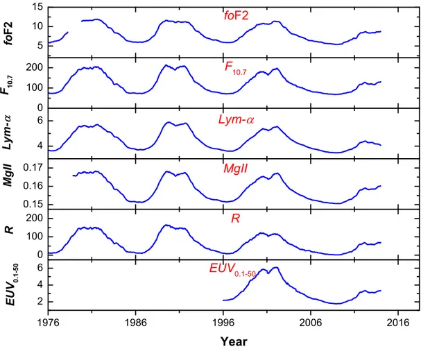
The study takes into account five widely used solar activity indices: 𝐹10.7, 𝐿𝑦𝑚-𝛼, 𝑀 𝑔𝐼𝐼, the

sunspots number 𝑅 and the solar irradiance in the EUV band 0.1-50 nm (𝐸𝑈 𝑉0.1−50). Every

index is described in detail, along with the available dataset and the sources from which solar indices data have been downloaded. The study is accomplished by considering foF2 values recorded at local noon (LT=UT+1h for Rome station). This choice was suggested by the fact that for every index only one daily value is available and measurements usually refer to local noon. Furthermore, studies of ionospheric long-term trends usually refer to local noon.

The main aim of this part of the work is to examine the foF2 dependence on solar activity, trying to discuss and solve specific problematics in order to obtain simple analytical relations to be used for ionospheric modeling. In order to obtain these results, a 1-year running mean is applied for both foF2 and solar indices. By using this methodology, it is possible to eliminate short-time ionospheric features, like those caused by geomagnetic disturbances, ionospheric seasonal and day-to-day variations, and (partially) reduce the saturation effect occurring at high solar activity. Furthermore, from “clean” (foF2 vs Solar Index ) plots it is easier to obtain accurate analytical formulae.

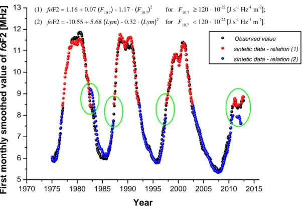
In the first part of the chapter the a priori supposed linear fit is tested to investigate whether it can still be considered as the best one. After that, the best fit is found using a residuals analysis. Then, the search for the best index, able to describe the variations of foF2 both globally (for the complete dataset 1976-2013) and for the last solar minimum (time interval January 2008-December 2009), is reported. The analysis is carried out by comparing ionosonde values with opportune synthetic datasets obtained for every solar index. Moreover, by introducing the 𝑅-Solomon parameter, it has been possible to compare the foF2 variations with the ones of indices for the whole cycle 23. This analysis gives the possibility to discuss another important issue: the search for the EUV solar radiation “best proxy”, which means to search for an index

(10)

Introduction

with a long available dataset that well approximates the variations of the solar radiation in EUV wavelengths. A section of the chapter is dedicated to additional analyses carried out during the work, providing some starting points for future studies. Specifically, the following issues are discussed: (1) systems of analytical relations; (2) foF2 (at 01 LT and 19 LT) vs Solar Index relationships for Rome station; (3) (NmF2 vs Solar Index ) and (hmF2 vs Solar Index ) relationships; (4) dependence of (foF2 vs Solar Index ) relationships on the geomagnetic activity.

Chapter 4 is an outline about the update of the SIRM model: it can be interesting to discuss how and whether the SIRM model can be improved according to the findings reported in Chapter 3. First, the theoretical aspects of the SIRM model are reported. Then, SIRM outputs for foF2 are compared with ionosonde values for the low solar activity years 2008 and 2009 to test its reliability in such particular conditions. After this preliminary analysis, the updated model, called SIRMPol, is introduced. SIRMPol foF2 outputs are then compared with both values measured by the ionosonde and calculated by SIRM, for both low solar activity (2008 and 2009) and very high solar activity (year 1958). In fact, as it is discussed in depth in the chapter, passing from SIRM to SIRMPol, more pronounced improvements are expected for high solar activity levels, when the saturation effect is dominant.

However, the most accurate description of the ionospheric parameters for a single station can be obtained by the development of opportune SSMs. The accuracy of these models increase with the availability of a long and continuous dataset. As previously underlined, for the Rome station a very robust dataset is available. For this reason, a SSM, namely Single Station Model for Rome (SSM-R), has been developed. SSM-R outputs for foF2 are compared with the ones given as output by SIRM and SIRMPol and values measured by the ionosonde for the aforementioned years at low and high solar activity. A complete updating of the SIRM model falls outside the main objectives of the present work and further analyses need to be carried out. Nevertheless, the preliminary results described in this chapter give the possibility to list several useful guidelines for a future updating of the SIRM, which are reported at the end of the chapter.

Chapter 5 is about the analysis of the recent solar minima and the investigation of the IRI-2012 reliability, at mid- and low-latitude stations. In this part of the work, data from four

ionospheric stations are used: Rome (41.8∘N, 12.5∘E, geomagnetic latitude 41.7∘N, Italy),

Gi-bilmanna (37.9∘N, 14.0∘E, geomagnetic latitude 37.6∘N, Italy), S˜ao Jos´e dos Campos (23.1∘S,

314.5∘E, geomagnetic latitude 19.8∘S, Brazil), and Tucum´an (26.9∘S, 294.6∘E, geomagnetic

lati-tude 17.2∘S, Argentina). Rome and Gibilmanna are descriptive of the mid-latitude ionosphere,

while São José dos Campos and Tucumán represent low-latitude stations located in an

ionosp-herically critical position, being close to the south crest of the Equatorial Ionization Anomaly.

Rome, Gibilmanna, and Tucum´an stations are all equipped with an AIS-INGV (Advanced

Ionospheric Sounder-INGV ) ionosonde, the S˜ao Jos`e dos Campos station is equipped with a

CADI (Canadian Advanced Digital Ionosonde) ionosonde, and corresponding data related to recent minima have been all validated, which has generated a very reliable dataset. The analysis concerns the electron density peak NmF2 and the height hmF2 at which it is reached. NmF2 has been obtained from validated foF2 values, using the plasma frequency formula; hmF2 has been obtained using Shimazaki and D55 analytical relations. However, for hmF2 a preliminary study has been carried out, comparing values from analytical relations with those from iono-gram inversions, in order to understand which is the relation that gives the most reliable values for a definite period.

The particularity of the last solar minimum is emphasized by an inter-minima comparison for

(11)

Introduction

both NmF2 and hmF2. Moreover, the reliability of the outputs given by the IRI-2012 model is tested for both parameters, for low solar activity, by comparing them with measured ones. A comparison between the results obtained at mid latitudes with the ones inferred at low latitudes for both the inter-minima comparison and the IRI-2012 reliability is also carried out.

The most important goals of this work can be summarized as follows:

1. To use the long and continuous dataset recorded at the ionospheric station of Rome to study the relations (foF2 vs Solar Index ):

∙ To observe whether the a priori supposed linear relation is valid or there have been changes owing to the last solar minimum;

∙ To find the best fit and index to describe the foF2 variations;

2. To obtain useful guidelines for a future complete update of the regional SIRM model and to develop a reliable SSM for the Rome station;

3. To evaluate the main behaviors of the ionosphere for the last solar minimum, making a comparison with the previous minima, for NmF2 and hmF2;

4. To evaluate the IRI outputs for the last solar minimum, making a comparison with the previous minima.

The results obtained and possible future analyses related to the present work are the subject of the “Conclusions and future developments” section.

Two papers have been extracted from the present work and accepted for publication in international journals. The first paper is based on the work described in Chapter 3:

Perna, L., Pezzopane, M., 2016. foF2 vs solar indices for the Rome station: Looking for the best general relation which is able to describe the anomalous minimum between cycles 23 and

24. Journal of Atmospheric Solar-Terrestrial Physics 148, 13-21, http://dx.doi.org/10.1016/j.

jastp.2016.08.003.

The second paper (in press) is based on the work reported in Chapter 5:

Perna, L., Pezzopane, M., Ezquer, R., Cabrera, M., Baskaradas, J. A., 2016. NmF2 trends at low and mid latitudes for the recent solar minima and comparison with IRI-2012 model.

Advances in Space Research, http://dx.doi.org/10.1016/j.asr.2016.09.025.

The front pages of both papers are attached after the “Conclusions and future developments” section.

The Acknowledgements and Bibliography are reported at the end of the thesis.

(12)

(13)

Chapter 1 The Terrestrial Ionosphere

Introduction

The term ionosphere usually identifies the part of the terrestrial atmosphere included between 50 and 500 km of height, that is between the stratopause and the termopause. The main feature of the ionosphere is the presence of free electrons and ions in a quantity that strongly influences the radio wave propagation.

The first hypothesis about the existence of the ionosphere can be found at the beginning of the XIX century, when Carl Gauss and Balfour Stewart hypothesized the existence of atmos-pheric electric currents in order to explain the observed variations of the terrestrial magnetic field. The definitive proof of the existence of the ionosphere was given on 12 December 1901, when Guglielmo Marconi established a radio link between the city of Poldhu (in the UK) and the Canadian city of St. John’s. At that time, the theory considered only a straight-line pro-pagation, so the Marconi’s experiment could be explained only considering the possibility of a reflection in the atmosphere. In 1902, A. E. Kennelly and O. Heaviside suggested the existence of an ionized layer in the atmosphere, able to deviate and reflect waves in radio wavelength ranges. Lee de Forest and L. F. Fuller, members of the Federal Telegraph Company of San Francisco, between 1912 and 1914, made the first measures about the height of this layer, but unfortunately the corresponding results are not well known. The first available measures are the ones of E. V. Appleton and M. A. F. Barnett (UK, 1924), who with an interferometric methodology found a reflection height of ∼92 km.

R. A. Watson-Watt suggested the name ‘ionosphere’ for the first time in a letter sent to the United Kingdom Radio Research Board on 8 November 1926. At the same time, Appleton started using the same term when writing a letter to J. A. Ratcliffe on 2 November 1926:

‘For the ionised part of the upper atmosphere I think the terms ionosphere or elec-trosphere might be useful. Which do you prefer?’

Nevertheless, the term ionosphere does not appear in literature until the 1929, when Watson-Watt at the Symond Memorial Lecture of the Royal Meteorological Society said:

‘It might be permissible to call it the Belfour-Stewart-Fitzgerald-Heaviside-Kennelly-Zenneck-Schuster- Eccles-Larmor-Appleton space, but something less direct is desi-rable. I have suggested the name ionosphere to make a systematic group troposphere, stratosphere, ionosphere, but meanwhile the term ‘upper conducting layers’ seems to hold the field’.

(14)

2 Chapter 1. The Terrestrial Ionosphere

After the 1932, the term proposed by Watson-Watt started to be used frequently in lite-rature, stopping a long discussion about the name of this layer that, in the previous years, had also been called upper reflection surface, conducting layer, Heaviside layer, day (or night ) effect from Marconi experiment, Kennelly-Heaviside layer and so on. A series of curiosities and anecdotes about the born of the name ionosphere can be found in Gillmor (1976).

The magnetoionic theory, the study of the propagation of electromagnetic waves in an ionized mean immersed in the terrestrial magnetic field, started being of great interest in particular since the beginning of the XX century. The most relevant results were obtained by Appleton that won the Nobel prize in 1947 for the discovery of the ionospheric layers and for his contribute to the magnetoionic theory.

The importance of the study of the ionosphere can be found in a series of aspects, the most important of which is that it significantly influences the communications Earth-Earth, Earth-satellite and satellite-satellite. Moreover, the ionosphere is strongly affected by the solar activity variations, and it is then strictly connected to the interactions between the Sun and the Earth.

This first chapter focuses on a general description and introduction of the main ionospheric features, with particular attention to the ones useful for the development of this work.

In the first section of this chapter, a description of the formation and vertical structure of the ionosphere will be reported. The second section will be instead devoted to the ionospheric variability, with a focus on the strong influence that the solar activity has on the ionospheric plasma. A brief review of the vertical ionospheric sounding technique is carried out in the last section.

1.1 Formation and vertical structure of the ionosphere

The ionosphere can be considered a low-density plasma, with an ionized component (ions and free electrons) representing a smaller fraction than the neutral one, so we can consider it a minority plasma. This kind of plasma, immersed into the terrestrial magnetic field, is called magnetoplasma.

The ionosphere forms due to the interaction between the radiation coming from the Sun and the high layers of the terrestrial atmosphere. The differential interaction of the radiation with the different atmospheric chemical species is responsible for the typical stratification of the ionosphere.

The main parameter characterizing a plasma is its plasma frequency, that represents the oscillation frequency of the electrons with respect to the fixed ions, when moved from a stable state position.

Considering a unidimensional configuration in which the electrons move a distance 𝑥 from the fixed ions, neglecting the thermal agitation and considering an infinite layer, under the action

of a disturbing electric field E, the restoring force due to the induced electric field Ei has the

intensity: 𝑒Ei = 𝑒 𝜎 𝜖0 ^ x = 𝑒𝑁 𝑒𝑥 𝜖0 ^ x, (1.1)

where Ei = 𝜎/𝜖0 is the electric field of an electrical double layer, 𝜎 = 𝑁 𝑒𝑥 is the superficial

(15)

1.1. Formation and vertical structure of the ionosphere 3

of the electron. The momentum equation for the electron of mass 𝑚 is then:

d2x

d𝑡2 +

𝑁 𝑒2 𝑚𝜖0

x = 0, (1.2)

which is the equation of an harmonic oscillator of which the angular frequency is:

𝜔𝑁 =

√︃ 𝑁 𝑒2 𝑚𝜖0

. (1.3)

Considering that 𝜔𝑁 = 2𝜋𝑓𝑁, the plasma frequency is then:

𝑓𝑁 = √︃ 𝑁 𝑒2 4𝜋2_𝑚𝜖 0 . (1.4)

The value of 𝑓𝑁 is crucial to determine the frequency usable for a radio communication.

The vertical structure of the ionosphere is caused by the counterpoised trend between the ionizing solar radiation (increasing outward) and the atmospheric density (increasing inward). Moreover, the differential interaction of the various chemical species with the solar radiation causes the formation of relative maxima of electron density in the profile. These maxima individuate the ionospheric layers. Figure 1.1 shows typical daytime and nighttime electron density profiles at mid latitude and for low solar activity (sunspot number 𝑅=0), where the F, E and D regions are pointed out.

The most important parameter characterizing an ionospheric layer is its critical frequency. If in the equation (1.4) we substitute the electron density 𝑁 with an electron density relative

maximum 𝑁mi, we obtain 𝑓𝑁 mi that represents the maximum frequency vertically reflected

by the ionospheric layer i. At each ionospheric layer is associated a critical frequency, with a simple notation; for example foE represents the critical frequency of the E region, foF2 the critical frequency of the F2 region and so on. The critical frequency foF2 is the most important ionospheric parameter and represents the maximum frequency vertically reflected by the ionosphere.

1.1.1 Processes involved in the formation of the ionosphere

The free electrons represent the main cause for the ionospheric reflection of radio waves, so the electron density value and its variations are of primary importance. The variation of 𝑁 with the time can be expressed using the electronic equilibrium equation:

d𝑁

d𝑡 = 𝑞(𝑡, X) − 𝑙(𝑡, X) + 𝑑(𝑡, X). (1.5)

The parameters 𝑞, 𝑙 and 𝑑 represent the production rate, disappearing rate and transport rate for electrons in the unity of time and volume, respectively. As equation (1.5) shows, the rate d𝑁 /d𝑡 depends also on the position X.

The main mechanism causing the production of free electrons is the photoionization due to the solar radiation. At mid and low latitudes the photoionization can be considered the only mechanism responsible for the formation of the ionosphere, meanwhile at polar zones other mechanisms such as the transport cannot be neglected.

(16)

Figure 1.1: Typical day- and night-time electron density profile at mid latitude, for low solar activity. The ionospheric D, E and F regions are highlighted on the right.

species, ℎ is the Planck constant, and 𝜈 the wave frequency of the Sun radiation; the ionization

is possible only if ℎ𝜈 ≥ 𝐸𝑖, where 𝐸𝑖 is the energy of ionization for the generic species 𝑖.

The photoionization cross section 𝜎 is introduced to consider the stochastic character of the process, depending on the wavelength 𝜆 of the incident radiation and on the particular species

𝐴𝑖. If 𝐼 is the intensity of the radiation and 𝑛 the density of a specific atomic species, we can

write the production rate 𝑞 as:

𝑞 = 𝜎(𝜆, 𝐴𝑖)𝑛𝐼. (1.6)

The main ionizing radiations coming from the Sun are those falling in the Ultra Violet wave-length range of 10-400 nm, and in the X-ray wavewave-length range of 0.1-10 nm.

The loss of electrons is due to two main mechanisms: recombination and attachment. The recombination consists in the interaction between positive ions and electrons, to form

neutral atoms and release energy (𝐴+ + 𝑒− → 𝐴 + Energy). Introducing the coefficient of

recombination 𝛾 (expressed in [m3/sec]), the probability of recombination will be:

𝑙r = 𝛾𝑁 𝐴+. (1.7)

The attachment consists in the interaction between neutral atoms and electrons, to form

nega-tive ions and release energy (𝐴 + 𝑒− → 𝐴−_{+ Energy). Introducing the coefficient of attachment}

𝛿 (expressed in [m3/sec]), the probability of the attachment will be:

𝑙a = 𝛿𝑁 𝐴. (1.8)

In this simple treatise, we consider 𝛿 and 𝛾 constants and do not take into account the disso-ciative recombination phenomenon.

(17)

1.1. Formation and vertical structure of the ionosphere 5

Local variations of 𝑁 that cannot be ascribed to photoionization or recombination are due to transport mechanisms, such as diffusion, thermal transport and turbulence.

The transport rate can be then expressed as:

𝑑 = 𝜕𝐷 𝜕ℎ (︁𝜕𝑁 𝜕ℎ + 𝑁 𝑇 𝜕𝑇 𝜕ℎ + 𝐺 𝑁 𝐻 )︁ − 𝑑𝑖𝑣(𝑁 V), (1.9)

where 𝐷 is the diffusive transport coefficient, 𝐺 is the gravitational transport coefficient, 𝑇 the absolute temperature, 𝐻 the scale height, ℎ the height and V the velocity field.

Introducing equations (1.6)-(1.9) in equation (1.5), we obtain d𝑁 d𝑡 = ∑︁ 𝑖 𝜎(𝜆, 𝐴𝑖)𝑛𝑖𝐼 − ∑︁ 𝑖 𝛾𝑖𝑁 [𝐴+𝑖 ] − ∑︁ 𝑖 𝛿𝑖𝑁 [𝐴𝑖] + 𝑑. (1.10)

Introducing into the (1.10) the effective recombination coefficient (𝛼 = Σ𝑖𝛾𝑖), the effective

atta-chment coefficient (𝛽 = Σ𝑖𝛿𝑖[𝐴𝑖]), and assuming [𝐴+𝑖 ] = 𝑁

+_{, the final version of the electronic}

equilibrium equation can be written as: d𝑁

d𝑡 = 𝑞 − 𝛼𝑁 𝑁

+_{− 𝛽𝑁 + 𝑑.} _(1.11)

1.1.2 Ionospheric layers and main parameters

As shown in Figure 1.1, the electronic density varies with the height being characterized by relative maxima. Every relative maximum identifies and characterizes a specific ionospheric region:

∙ D region; ∙ E region; ∙ F region.

The D region is the lowest one and extends from 50 to 90 km, with an electron density peak

of ∼109 _m-3 _{at ∼80 km. Sometimes a lower layer, called C layer, can be visible at heights of}

65-70 km. The D region is not useful for radio communication because of the very low electron density; instead it represents the most absorbing layer, because of the highest value of the quantity 𝑁 𝜐, where 𝜐 is the collisional frequency. The D and C regions are only visible during daytime hours.

The E region, characterized by heavy ions (O+₂ and NO+), extends from 90 to 150 km,

with an electron density peak of ∼1011 m-3 _{at ∼120 km. A peculiar feature of this layer is}

the appearance of random and fast stratifications (0.2-2 km thick) with 𝑁 > 1012 m-3, called

sporadic E layers. The E region is mainly a typical daytime region, even though a light nighttime

stratification (𝑁 ∼ 5 · 109 _m-3_{) is observed.}

The region between 150 and 500 km, dominated by light ions (O+, H+, He+, N+), represents

the F region, of which the electron density maximum of 𝑁 ∼ 5 · 1012_m-3_{is reached at ∼300 km.}

During daytime hours, the F region can be split in two different layers: the 𝐹1 layer and the 𝐹2

layer. The F1 layer is characterized by an electron density maximum of ∼1011 m-3 at ∼180 km,

with a predominance of ions O+_{, and it is a layer typically diurnal. The F}

2 layer, formed for

the 95% of ions O+_{, is the most important layer for radio communication purposes, with an}

(18)

During the nighttime it is visible a unique F region with an electron density peak of ∼7·1010m-3

at ∼300 km.

D, E and F1 layers can be considered 𝛼-Chapman layers, that means diurnal layers with

maximum electron density at midday and in summer; the F2 layer instead can be considered a Bradbury layer, with the electron density monotonically decreasing with the height, after reaching its maximum (Dominici, 1971).

As mentioned, the F region is the most important for radio communication purposes. The-refore, the critical frequency foF2 represents the most important ionospheric parameter. It represents the maximum frequency reflected by the ionosphere for a radio wave transmitted vertically.

foF2 is linked to the maximum electron density NmF2 of the vertical profile, in fact from

equation (1.4) we obtain that NmF2 [m-3_{]= 1.24·10}10_{(foF2 [MHz])}2_{. The height at which}

NmF2 is reached is indicated as hmF2. foF2 is easily deducted, manually or automatically, directly from an ionogram. To calculate hmF2 the situation is quite different and complex. Only in the last years, the calculation of this value has become a routine operation for

auto-matic scaling systems which perform an inversion of the ionogram1_{, a necessary step to obtain}

hmF2. Alternatively, as it will be explained in more detail in Section 1.3.2, it is possible to use analytical relations that include other ionospheric parameters such as foE or the Maximum Usable Frequency MUF (3000)F2, which represents the maximum frequency usable for a radio communication between two points at a distance of 3000 km. Also foE and MUF (3000)F2 can be easily deducted from an ionogram.

1.2 Variability of the ionosphere

The ionosphere is a very variable system. It is strongly influenced by a great number of

phenomena linked to the solar and geomagnetic activity, the seasons, the hour of the day, the latitude, and the longitude. A complete discussion on the ionospheric variability is out of the scope of this work, nevertheless in this section ionospheric features that will be useful to the comprehension of the next chapters will be discussed and introduced.

As mentioned, the ionosphere forms owing to the interaction between the solar radiation and the terrestrial atmosphere. By virtue of this, the solar activity represents the main controller of the ionospheric variability. Consequently, the ionospheric parameters show trends that follow quite well the indices representing the solar activity level. In Figure 1.2 are plotted the 1-year

running mean of the index 𝐹10.7 (representing the solar flux at 10.7 cm and described in detail

in Section 3.1), that represents a widely used indicator of solar activity, and the 1-year running mean of validated values of foF2, observed at 12 LT at the ionospheric station of Rome, from the 1 January 1976 to the 31 December 2014, a period of time covering partially the solar cycle 24 and completely the solar cycles 21, 22 and 23. It is visible the similar trend of the two parameters, which means that there is a strong correlation between the solar activity variations and the response of the ionosphere. In fact, the parameter foF2 follows the increase/decrease of the solar activity, with higher/lower values for high/low solar activity. Furthermore, Figure 1.2

suggests a quasi-linear relation between 𝐹10.7 and foF2. This will be the object of the study

described in Chapter 3.

An important ionospheric feature, linked to the dependence of the ionosphere on the solar activity, is the saturation effect observed for high solar activity (Liu et al., 2003, 2006, 2011b;

(19)

1.2. Variability of the ionosphere 7 1 9 7 6 1 9 8 1 1 9 8 6 1 9 9 1 1 9 9 6 2 0 0 1 2 0 0 6 2 0 1 1 2 0 1 6 6 0 8 0 1 0 0 1 2 0 1 4 0 1 6 0 1 8 0 2 0 0 2 2 0 2 4 0 2 6 0 1 -y e a r ru n n in g m e a n F 1 0 .7 1 0 -2 2 [ J H z -1 s -1 m -2 ] Y e a r 2 1 2 2 2 3 2 4 5 6 7 8 9 1 0 1 1 1 2 1 3 1 4 1 -y e a r ru n n in g m e a n f o F 2 [ M H z ]

Figure 1.2: 1-year running mean of the solar index 𝐹10.7(black line) and foF2 (12 LT in Rome, blue

line), from 1 January 1976 to 31 December 2013.

Ma et al., 2009), for which after a definite level of solar activity, the parameter foF2 does not increase anymore as the solar activity increases. This effect is particularly visible when using mean or median values for both the ionospheric parameter and the solar activity index, and shows a seasonal dependence, with a more pronounced saturation from April to September in the North hemisphere, at all the hours of the day.

Figure 1.3 shows the monthly median values of foF2 (at local noon in Rome) as a function

of the 12-month running mean of the monthly mean sunspots number 𝑅12, for May, from 1958

to 2007. The red dashed circle highlights the values affected by the saturation. For the trend

foF2 vs 𝑅12, the saturation is visible after a level of ∼150 for 𝑅12.

The trends between foF2 and solar activity indices can be subjected to another important phenomenon, linked most probably to the geomagnetic activity level, the hysteresis effect (Kane, 1992; Mikhailov and Mikhailov, 1995; Liu et al., 2006; Rao and Rao, 1969; Triskova and Chum, 1996).

The hysteresis effect causes two different values of foF2 for the ascending and descending phase of the same solar cycle, in correspondence of the same level of solar activity. Mikhailov and Mikhailov (1995) postulated that the hysteresis is associated with differences in the geomagnetic activity during the ascending and descending phases of a solar cycle. Nevertheless, there is not yet an accepted explanation for the hysteresis effect (Liu et al., 2011b). In Figure 1.4 is shown the clear hysteresis effect observed in the trend foF2 (12 LT) vs 𝐿𝑦𝑚-𝛼 (see Section 3.1 for a detailed description of this solar index), for the solar cycle 23.

(20)

8 Chapter 1. The Terrestrial Ionosphere 0 2 5 5 0 7 5 1 0 0 1 2 5 1 5 0 1 7 5 2 0 0 2 2 5 5 6 7 8 9 1 0 1 1 1 2 M o n th ly m e d ia n f o F 2 [ M H z ] R _{1 2}

Figure 1.3: Monthly median values of foF2 as recorded at Rome in May, at local noon, from 1958 to 2007 as a function of 𝑅12. The red dashed circle highlights data affected by the saturation effect.

visible only for mid solar activity, and not for low and high solar activity.

Both the saturation and the hysteresis effect have a great influence on the relation between the ionospheric parameter foF2 and the indices of solar activity. As it will be discussed in Chapter 3, the research of the best index to describe the variations of foF2 has to take into account these two effects.

Very important is the seasonal ionospheric variation, linked to the Sun-Earth interaction. In particular, for this study, we will consider the winter anomaly and the semiannual anomaly (Ezquer et al., 2014; Dominici, 1971; Chen and Liu, 2010; Liu et al., 2012; Rishbeth and Setty, 1961; Rishbeth et al., 2000; Yu et al., 2004; Rishbeth and Garriot, 1969; Yonezawa and Arima, 1959; Yonezawa, 1967, 1971; Torr and Torr, 1973).

The winter anomaly consists in the observation of values of the electron density peak NmF2 (or analogously of the critical frequency foF2) at local noon that are lower in summer than in winter.

It has been proposed that this anomaly is related to changes in the neutral composition of the atmosphere, generated by heating in the summer hemisphere and a subsequent convection of lighter neutral elements towards the winter sector, which causes changes in the ratio of [O]/[N2] in both hemispheres (Rishbeth and Setty, 1961; Johnson, 1964; Torr and Torr, 1973). In Figure 1.5 the effect is clearly visible, with values of NmF2 around the local noon that are significantly lower in June (in red) than in December (in blue). The latitude and the solar activity influence the winter anomaly, which is less visible at low latitude, in the South hemisphere and for low solar activity.

(21)

1.2. Variability of the ionosphere 9 3.0 3.5 4.0 4.5 5.0 5.5 6.0 5 6 7 8 9 10 11 12 13

Ascending phase cycle 23 Descending phase cycle 23

f o F 2 [ M H z ] Lym- 10 11 photons [s -1 cm -2 ]

Figure 1.4: foF2 vs 𝐿𝑦𝑚-𝛼 for the ascending phase (full circles) and descending phase (empty circles) of the solar cycle 23. The vertical arrows highlight the hysteresis effect.

5.0x10 11 1.0x10 12 1.5x10 12 2.0x10 12 2.5x10 12 April June October December M e d i a n N m F 2 [ m -3 ] 1990 1991 00 03 06 09 12 15 18 21 24 5.0x10 11 1.0x10 12 1.5x10 12 2.0x10 12 2.5x10 12 M e d i a n N m F 2 [ m -3 ] Local Time 2001 00 03 06 09 12 15 18 21 24 2002 Local Time

Figure 1.5: Monthly median values of NmF2 as recorded at Rome in April, June, October and December for the years of maximum activity 1990-1991 (max of solar cycle 22) and 2001-2002 (max of solar cycle 23).

(22)

Another important feature visible in Figure 1.5 is the semiannual anomaly for which va-lues of NmF2 are greater around equinoxes (April and October) than around solstices (June and December). Also this effect depends on the latitude, being more visible at low latitudes (Rishbeth and Garriot, 1969; Ezquer et al., 2014). Furthermore, the amplitude of the semi-annual anomaly is larger in years of solar maximum than in years of solar minimum (Ma et al., 2003). Several mechanisms have been proposed to explain this anomaly. Yonezawa (1971) proposed that it is related with the variation of the upper atmosphere temperature. Torr and Torr (1973) suggested that it is caused by the semi-annual variation of neutral densities asso-ciated with the geomagnetic and aurora activity. Mayr and Mahajan (1971) showed that the anomaly requires significant variation in the neutral composition at lower height. Ma et al. (2003) suggested that the semi-annual variation of the diurnal tide in the lower thermosphere induces the semi-annual variation of the amplitude of the equatorial electrojet, thus causing the semi-annual anomaly at low latitude.

All the phenomena introduced in this section will be considered in the development of the work, and will be recalled in the next chapters. In particular, the saturation and hysteresis effects strongly affect the research of the best solar index to describe the variations of foF2. The winter and semiannual anomalies will be instead considered in the inter-minima comparison, owing to their dependence on solar activity level.

1.3 Ionospheric vertical sounding: a brief review

In order to determine the parameters characterizing the ionosphere, different typologies of ionospheric sounding can be used. The ionospheric soundings can be divided in three main branches: active, passive and perturbative. The active methodologies are the most widely used and are: the vertical and oblique sounding, the ground scatter radar and the incoherent scatter radar. Passive measures are those performed by riometers, and those exploiting the GPS constellation. Examples of measures performed with a perturbative methodology are the HF heating and the cross modulation. In this section we will treat the most used technique: the vertical ionospheric sounding. In Section 1.3.1 an introduction about the radar technique will be reported, while Section 1.3.2 will be devoted to the description of the main features of an ionogram.

1.3.1 Radar technique

The vertical sounding is based on the Radar Theory (Radio Detection and Ranging). Consi-dering the ionosphere as an infinite and perfectly reflecting layer, it is possible to record the

travel time of a radio wave (in the High Frequency (HF)2 _{band) sent vertically and reflected by}

the ionosphere. Assuming the wave travelling at the speed of light 𝑐, measuring the travel time

𝑡 it is possible to obtain the virtual height of reflection ℎ′, that is ℎ′ = 𝑐𝑡/2. As a consequence,

the result of an ionospheric vertical sounding will be a plot of ℎ′ as a function of the frequency

𝑓 . This plot is called ionogram and from it the most important ionospheric parameters can be inferred, as it will be described in the next section.

To understand the meaning of an ionogram, we need to obtain the radar equation and adapt it to the special case of the ionosphere.

(23)

1.3. Ionospheric vertical sounding: a brief review 11

In the simple case of a bi-static radar, with gain of the antennas 𝐺T (transmitter TX) and

𝐺R (receiver RX) at a distance 𝑟, from the TX antenna the target will receive a power flux

𝜑i =

𝑃rad𝐺T

4𝜋𝑟2 , (1.12)

where 𝑃rad is the emitted power.

Owing to the power diffusion of the target 𝜎𝜑i, being 𝜎 the radar cross section, the flux turning

back to the radar is:

𝜎𝜑i

4𝜋𝑟2 =

𝑃rad𝐺T𝜎

(4𝜋𝑟2₎2 . (1.13)

If 𝐴eff is the effective surface of the receiver RX, the corresponding captured power can be

expressed as:

𝑃r =

𝑃rad𝐺T𝜎𝐴eff

(4𝜋𝑟2₎2 . (1.14)

Using the relation 𝐴eff = (𝜆𝐺R)/(4𝜋), the relation (1.14) becomes:

𝑃r =

𝜆2_𝐺

T𝐺R𝜎𝑃rad

(4𝜋)3_𝑟4 , (1.15)

that represents the explicit form of the radar equation.

The vertical ionospheric sounding can be understood considering a particular case of the equation (1.15), which for the ionosphere can be expressed as:

𝑃r=

(𝜆𝐺)2𝑃rad

(4𝜋𝑟)2_𝐿 , (1.16)

with 𝐿 attenuation of the signal, and considering the ionosphere as an infinite reflecting layer,

which means 𝐺 = 𝐺T = 𝐺R.

The sounding depends on the variations of the electron density 𝑁 with the height. By neglecting both the magnetic field and collisions, the reflection occurs at heights where the

emitted frequency 𝑓 equalizes the plasma frequency 𝑓𝑁. The plasma frequency depends on 𝑁

and consequently on the real height ℎ and according to (1.4) is expressed as:

𝑓𝑁(ℎ) = √︃ 𝑁 (ℎ)𝑒2 4𝜋2_𝑚𝜖 0 . (1.17)

By virtue of the equation (1.17), different frequencies will be reflected at different heights and so will turn back to the Earth with different delay times. From the delay time (or travel

time) measured it is possible to obtain ℎ′ and then the ionogram trace that, as mentioned, is a

plot of ℎ′as a function of the emitted frequency.

For a vertical sounding, usually the frequency range is between 1 and 20 MHz, depending on the latitude of the ionospheric station, with a frequency step of 25, 50 or 100 kHz. The height resolution is less than 5 km, with minimum and maximum heights of about 90 and 600 km respectively, covering all the ionospheric regions of interest.

(24)

Figure 1.6: Example of ionograms recorded at Tucum´an, Argentina, (top) on 9 August 2010 at 22:05 LT, and (bottom) on 9 September 2010 at 10:25 LT.

1.3.2 Main ionogram features

As previously said, an ionogram is the output of a vertical ionospheric sounding.

Figure 1.6 shows two typical ionogram traces for nighttime and daytime hours. The

iono-grams have been recorded at the ionospheric station of Tucum´an (Argentina) on 9 August 2010

at 22:05 LT and on 9 September 2010 at 10:25 LT, respectively, and give us the possibility to make a comparison between the daytime and nighttime ionosphere. In the top ionogram, it is possible to distinguish only one cusp that individuates the nighttime F region. Instead, in the

bottom ionogram are visible three cusps that individuate, as the frequency increases, the E, F1

and F2 layers.

At every cusp corresponds a critical frequency of an ionospheric layer. In fact, for a vertical

travelling wave at constant velocity 𝑐, the equivalent height of reflection ℎ′ can be expressed as:

ℎ′ = 𝑐𝑇 2 ∫︁ 𝑇 0 𝑐 2d𝑡, (1.18)

(25)

𝑣gr = 𝑐/𝑛gr where 𝑛gr is the refraction group index, and if we introduce it in equation (1.18) we

obtain: ℎ′ = ∫︁ 𝑇 0 𝑛gr· 𝑣g 2 d𝑡. (1.19)

If dℎ is the infinitesimal height variation, considering 𝑣gr = 2dℎ/d𝑡, the equation (1.19)

becomes:

ℎ′ = ∫︁ ℎr

0

𝑛grdℎ, (1.20)

where ℎr is the real reflection height. By taking a unitary refraction index under a height of

ℎ0, considered as the lower limit of the ionosphere, equation (1.20) can be rewritten as:

ℎ′ = ℎ0 +

∫︁ ℎr ℎ0

𝑛grdℎ, (1.21)

In the simplest case of no collisions and no magnetic field, the phase refraction index 𝑛 can be written as:

𝑛2 = 1 − 𝑋 = 1 − 𝑓

2 𝑁

𝑓2, (1.22)

and the relationship 𝑛gr · 𝑛 = 1 is valid (for more details see Ratcliffe (1959)). So, equation

(1.21) can be also written as:

ℎ′ = ℎ0+ ∫︁ ℎr ℎ0 𝑛grdℎ = ℎ0+ ∫︁ 𝑓𝑁=𝑓 𝑓𝑁=0 𝑛gr(𝑓𝑁) (︂ dℎ d𝑓𝑁 )︂ d𝑓𝑁. (1.23)

The equation (1.23) shows that for ℎ′ there will be an infinite value when the ratio d𝑓𝑁/dℎ

goes to zero. This situation is verified only when a relative maximum of the electron density 𝑁 occurs, and this explains why a cusp is observed in the ionogram in correspondence of a relative maximum of the electron density in the vertical profile, that is in correspondence of a critical frequency.

It is quite simple now to understand how the critical frequencies of the different ionospheric layers can be easily obtained from an ionogram.

With reference to Figure 1.7, it is possible to see how at every cusp corresponds the critical frequency of an ionospheric layer; in fact, the vertical asymptotes occur exactly in correspon-dence of critical frequencies. At the same time, the horizontal asymptotes individuate the virtual heights of reflection of the base of the different ionospheric layers.

So, it is clear now how the main ionospheric parameters can be validated from an ionogram, in particular the critical frequency of the F2 layer, foF2. As it was already said, foF2 is related to the maximum electron density of the vertical profile, NmF2.

An important parameter that cannot be directly calculated from an ionogram is the height of the maximum electron density, ℎ𝑚F2. To obtain this ionospheric parameter it is necessary

to perform an inversion of the ionogram, passing from the ionogram trace ℎ′(𝑓 ) to the vertical

electron density profile 𝑁 (ℎ). This passage is also called reduction to the real heights. Usually, to invert ionograms methodologies based on Target functions or polynomial inversion are used.

A Target Function is defined as follow:

Γ = ∫︁

(26)

Figure 1.7: Critical frequencies and virtual reflection heights of the base of different ionospheric layers as obtained from an ionogram. The vertical asymptotes (in red) individuate the critical frequencies, while the horizontal asymptotes (in green) individuate the equivalent reflection heights of the base of layers. The ionogram was recorded in Gibilmanna on 19 May 2011 at 15:30 LT.

with ℎ′_a(𝑓 ) representing a synthetic ionogram constructed “ad hoc”, starting from a specific

vertical electron density profile 𝑁 (ℎ). ℎ′_a(𝑓 ) can be expressed as:

ℎ′_a(𝑓 ) − ℎ0 = ∫︁ ℎr ℎ0 𝑛grdℎ = ∫︁ ℎr ℎ0 dℎ 𝑛 = ∫︁ ℎr ℎ0 dℎ √︁ 1 − _4𝜋𝑒22𝑁 (ℎ)_𝜖 0𝑚𝑓2 . (1.25)

Varying 𝑁 (ℎ), it is possible to minimize the value of the target function given by the equation (1.24). The synthetic profile for which the function is minimum will be the electron density profile associated to the ionogram.

Concerning the polynomial inversion, the most widely used program is POLAN, developed by John Titheridge. Detailed information about this program can be found in Titheridge (1985). Nevertheless, the use of POLAN requires an accurate ionogram validation, fixing various points on the trace that will be used for the inversion. It is clear that for long ionogram time series this methodology requires a long validation procedure and “clean” ionograms that are not always available.

However, in the years, analytical formulations to obtain an approximate value for hmF2 have been developed (see Ulich (2000) for a very good summary of them). Among them, in this work, we are mostly interested in the Shimazaki formula (Shimazaki, 1955) and the Dudeney formula D55 (Dudeney, 1974).

The Shimazaki formula is expressed by the following equation,

ℎ𝑚F2[km] = 1490 · 𝑓 𝑜F2[MHz]

𝑀 𝑈 𝐹 (3000)F2 − 176. (1.26)

The formula (1.26) is very simple and is calculable for every given time of the day, because only the ionospheric parameters foF2 and MUF are required.

(27)

The 𝐷55 formula is expressed by the following system of equations, ⎧ ⎪ ⎪ ⎨ ⎪ ⎪ ⎩ ℎ𝑚F2 = 1490 𝑀 + Δ𝑀 − 176, Δ𝑀 = 0.280 ± 0.009_{𝑓 𝑜F2} 𝑓 𝑜E − 1.200 − (0.028 ± 0.010). (1.27)

The D55 formula requires to know foF2 and foE, so its use is limited to daytime hours when foE is available.

In our study, before obtaining hmF2 for very long time periods by using (1.26) and (1.27), a preliminary phase to test their reliability was performed by comparing the corresponding values with those calculated by inversion methodologies of automatic scaling programs. As will be reported in Chapter 5, we found a good reliability of the Shimazaki formula for nighttime hours and for all the months, meanwhile the D55 formula is reliable during daytime hours, in particular for winter/autumn months, with bigger uncertainties for summer months.

(28)

(29)

Chapter 2 The particular minimum of the solar

cycle 23/24

Introduction

This work is focused on the last solar minimum, the minimum between the solar cycle 23 and the solar cycle 24 (minimum 23/24).

The great interest in the last minimum is due to the fact that the solar activity has been unusually low for a very long period including the years 2008-2009, that represent the years with the lowest solar activity, and partially the years 2007 and 2010.

Using as a solar activity indicator the observed number of sunspot, 527 days without sunspots have been observed for the period 2008-2009, while a mean of ∼300 days without sunspots characterized the last 10 solar minima. Furthermore, the solar cycle 23 lasted 12 years and 6 months, against a mean solar cycle duration of ∼11 years. Therefore, we are talking about a minimum that has come later than we expected and characterized by a very low and prolonged solar activity.

In the study of the ionosphere there is always an increasing interest in the analyses of the ionospheric plasma response for extreme conditions of solar activity (very high or very low). The last solar minimum gives us a natural unique window to study the ionosphere under conditions of extreme low solar activity. It is also particularly interesting to evaluate the response of the most widely used ionospheric models in such extreme conditions.

In this short chapter we will report the most relevant and interesting characteristics observed for the last solar minimum, highlighting at the same time why it is so interesting for ionospheric studies.

2.1 Main observed features of the minimum 23/24

The last minimum of solar activity, the minimum 23/24, was characterized by a very low and prolonged solar activity. This situation is very uncommon and offers us a unique natural window to study the ionospheric plasma response in such very particular conditions.

The Figure 2.1 shows the 1-year running mean for the sunspots number 𝑅. The complete solar cycles 21, 22 and 23 are shown until December 2014, covering partially the solar cycle 24. The plot shows interesting characteristics that are useful to understand the particularity

(30)

18 Chapter 2. The particular minimum of the solar cycle 23/24

of the last solar minimum. Focusing the attention on the sunspots number1, 176 days without

sunspots were observed for the years 1986-1987 that characterize the minimum of the solar cycle 21/22, with a duration of 10 years and 7 months for the cycle 21. For the years 1996-1997, which are the years of solar activity minimum of the cycle 22/23, 226 days without sunspots were observed, with a duration of 9 years and 8 months for the cycle 22. For the solar cycle 23, characterized by a duration of 12 years and 6 months, 527 days without sunspots were observed, only limiting the duration of the minimum to the years 2008-2009. Therefore, we are talking about a minimum that has come later than we expected and characterized by an extreme low and prolonged solar activity. As mentioned, it is important to note that the low solar activity can be considered particularly prolonged, because the period of uncommon low solar activity also interests partially the 2007 and the 2010. Nevertheless, the years 2008-2009 represent the deepest part of the minimum.

With reference to Chapter 1 and to the strong influence that the solar activity has on the ionospheric plasma, interesting and important responses are expected in the study of the main ionospheric parameters. In particular, it is very important to assess whether and how the relationships between the main ionospheric parameters and the most used solar indices are changed, being these relations essential to develop ionospheric models.

Figure 2.1: 1-year running mean of the sunspots number R for the last complete three solar cycles 21, 22 and 23. The solar cycle 24 is partially covered until December 2014.

1_{Data from SILSO (Sunspot Index and Long-Term Solar Observations, Royal Observatory of Belgium,}

(31)

2.1. Main observed features of the minimum 23/24 19

Figure 2.2: (top) 81-day average log-density at a fiducial altitude of 400 km, after removing seasonal and geomagnetic activity effects; (bottom) 81-day average for the solar index 𝐹10.7. The horizontal

black lines illustrate the differences between the cycle 23/24 and 22/23 minima (modified from Emmert et al. (2010)).

Emmert et al. (2010) used global-average thermospheric total mass density, derived from the drag effect on the orbits of many space objects, to study the behaviors of the thermosphere during the last solar minimum. They found that during the period 2007-2009 the thermospheric densities at an altitude of 400 km were the lowest observed in the 43-year (1967-2010) database, and were anomalously low, by 10-30%, compared with climatologically expected levels. They also found that the density anomalies appeared well before during the cycle 23/24 minimum, and are larger than what expected correspondingly to an enhanced thermospheric cooling caused

by increasing concentrations of CO2.

Figure 2.2 shows the 81-day averages for the log-density at 400 km and for the solar index

𝐹10.7, for the last four solar cycles; a comparison for the last two solar minima shows a decrease

of 28% in the log-density and of 3.7% in 𝐹10.7. The green dashed line individuates the trend

expected considering the previous solar minima, which can explains a decrease of 6% between the last two solar minima; so the observed decrease is much bigger than that expected, proofing the particularity of the last solar minimum.

Heelis et al. (2009) report results about the transition height O+_/H+ _{for the year of}

mini-mum 2008 measured by the satellite C/NOFS (Communications/Navigation Outage Forecasting

System) launched in April 2008. The O+/H+ transition height is a sensitive indicator of solar

extreme ultra violet ionizing flux and the dynamics of the topside ionosphere (MacPherson et al., 1998). Usually, the transition height resides near 450 km at night and rises to 850 km during daytime. The results show that for the latter half of 2008 this surface is much closer