SVMs for system identification: the linear case

UNIVERSITY

OF TRENTO

DIPARTIMENTO DI INGEGNERIA E SCIENZA DELL’INFORMAZIONE

38050 Povo – Trento (Italy), Via Sommarive 14

http://www.disi.unitn.it

SVMS FOR SYSTEM IDENTIFICATION: THE LINEAR CASE

Anna Marconato, Andrea Boni, Dario Petri and Johan Schoukens

August 2008

SVMs for system identification: the linear case

Anna Marconato

1

, Andrea Boni

1

, Dario Petri

1

, Johan Schoukens

2

1 _{DISI – University of Trento, via Sommarive 14, 38100 Trento, Italy}

E-mail: anna.marconato@disi.unitn.it

2

ELEC – Vrije Universiteit Brussel, Pleinlaan 2,1050 Brussels, Belgium

I. Introduction

In this work we deal with the application of Support Vector Machines for Regression (SVRs) to the problem of identifying linear dynamic systems on the basis of a set of Input/Output samples. Three different examples of simple linear systems will be considered, taking into account both non-recursive and recursive models. When defining the SVR estimating function, several examples of kernels will be employed, with emphasis on the ones that may be more appropriate for describing linear models. As a further step, the exact parameters of the model will be directly estimated from the Support Vector values resulting from the SVR training phase.

II. Support Vector Machines for system identification

SVRs, as other learning-from-examples algorithms, are based on a very simple principle: once you have collected a set of Input/Output measurementsZ =

{

x_i,y_i

}

_iN₌₁ a training phase is performed aimed at extracting all useful information from the available data. Thus, an estimating function f x( _i) is built that approximates the input-output relationship. Following the standard ε -SVR approach, errors are penalised, in a linear way, only outside a so-called insensitive zone, whose width is indicated by ε, while deviations smaller than ε are considered to be negligible [1]. The cost function is then defined by summing up all error contributions, and by taking into account a term describing the smoothness of the function.

This formulation of the SVR algorithm results in the definition of a constrained quadratic optimization problem where the function to be minimized turns out to be convex, therefore avoiding local minima problems (something that instead hampers other techniques, e.g. Artificial Neural Networks.)

The obtained SVR estimating function is the following:

q k f y _i SV i i + = =

∑

∈ ) , ( ) , ( ˆ x β β x x

Notice that not all the samples used during the training give a positive contribution, instead only a subset of the original dataset (the Support Vectors xi) is used for building the model [1]. Furthermore, suitable kernels are introduced in the

definition of the SVR function. Here we will try different kinds of kernel functions, including Gaussian, linear and triangular kernels, as will be discussed in depth in Section V.

The performance of the SVR function depends on a number of parameters (called hyperparameters) that need to be tuned in order to get the best possible model. Examples of these hyperparameters are the width ε of the insensitive zone, and specific parameters characterizing the kernel function. Here, as optimality criterion, we will consider an accuracy index, namely the Root Mean Square Error (RMSE) of the model with respect to the true output value. The optimal model is then chosen as the one giving the smallest RMSE in the training phase, and can then be tested on a set of previously unseen samples.

To explore the hyperparameters space during the model selection phase, we decided to exploit a technique based on Genetic Algorithms, which provide a faster and more efficient search tool when compared with the traditional grid search approach [2].

III. Considered examples of linear systems

The first linear system that we consider here is a first order discrete time system given by:

1 1 0 0 5 . 0 1 ) ( ), ( ) ( ) ( − − − = = z z z G with t u z G t y

resulting in the following expression:

) 1 ( 5 . 0 ) 1 ( ) 1 ( ) 1 ( ) (t =a⋅u t− +b⋅yt− =u t− + yt− y

that can be rewritten, introducing d as the number of past input samples, as:

∑

= − _{− + − −} = d k d k d t y k t u t y 1 1 ) 1 ( 5 . 0 ) ( 5 . 0 ) (

Having a look at the impulse response of the system, we notice that after 8 samples it is already less than 1/100 of the initial value. Therefore, we can choose to describe the system by taking into consideration 8 delayed input values as features, meaning that x is built as

[

u(t−1),K,u(t−8)

]

. Of course it will be necessary to accept a small error, since the system cannot be completely described in a non recursive way. In the following, we will refer to this example as “System A”.

Alternatively, a recursive model can be employed, building the feature vector x as

[

u(t−1),y(t−1)

]

. This will result in the second system used in this work (“System A_rec”).

A third example is given by another simple discrete time system, obtained considering the following transfer function:

2 1 0(z)=z− +0.5z−

G

The resulting linear system is formulated as follows (“System B”):

) 2 ( 5 . 0 ) 1 ( ) 2 ( ) 1 ( ) (t =a₁⋅u t− +a₂⋅u t− =u t− + u t− y

and can thus be perfectly described by 2 delayed input values, u(t−1),u(t−2).

Notice that, theoretically, in these simple cases, “System A_rec” and “System B” can be reconstructed knowing only 2 features.

In the following, when discussing the results obtained on these three different systems, we will address each case separately.

IV. Excitation signals and characteristics of datasets

As excitations, we decided to use, for all the considered systems, a Random Phase Multisine signal, characterised by the following equation:

∑

= + = F k k k f kt A t u 1 0 ) 2 cos( ) ( π ϕ

where f0 = 1/N, t = 1,...,N and φk is uniformly random distributed in [0,2π) [3]. For the training phase, the excitation signal is made of N =1024 samples, and F =125 (excited frequencies up to F⋅f0 =125⋅1/1024=0.12). Notice that the maximum excited frequency of the considered multisines is approximately equal to the cut-off frequency of system A, and nearly half the cut-off frequency of system B. Amplitudes Ak were normalized in order to have a root mean square value of the signal equal to 1.

For selecting the best model during the training phase, two different datasets need to be generated, a training set for building the SVR model and a validation set on which the performance can be evaluated. Here we chose training and validation sets both of size Ntraining = Nvalidation = 1024.

Once the best configuration of the hyperparameters is determined, the selected SVR model can be validated on a final test set, usually made of a very large number of samples in order to allow a more reliable estimate of the error. In this work, Ntest = 105 (the value of F is adjusted in order to obtain a multisine with the same frequency band as in the training).

The number of features will of course vary, depending on the specific model taken into consideration, as already explained in Section III.

V. Choice of the kernel function

In the SVR problem, so-called kernel functions are usually introduced, in a more general (nonlinear) framework, in order to express (in terms of inner products) the mapping from the original input space into another dot product space with much higher dimensionality. A widely common choice in many applications is the use of a Gaussian kernel function [4], expressed as:

2 ) , (x x =_e− xi−x k i γ

This kernel (along with other radial basis function kernels) is considered the most appropriate solution in all those cases when no further knowledge on the problem is available [5]. Notice here that parameter γ needs to be tuned in the model selection phase, since the choice of its value will heavily affect the performance of the SVR model.

Although the Gaussian kernel can be employed (with very good results, as we will see further on) also when reconstructing a linear relationship between the input and the output, a linear SVR estimating function seems, at least from a theoretical point of view, the most natural choice. To this aim, simple linear kernels are introduced [4]:

x x x x_i = _i⋅

k( , )

An appealing property of the linear kernel is that its formulation does not depend upon any parameter, making model selection a much simpler (and faster) procedure.

Another example of (piecewise) linear function that can be employed as kernel for SVR is the so-called triangular kernel [6]: x x x x_i =− _i− k( , )

It has been shown that the triangular kernel has the following interesting property: it makes the SVR function invariant to any scale of the data. Moreover, no tuning of extra parameters is needed [7].

A “rectified” version of the triangular kernel may also be considered:

(

)

otherwise C if C C k _i i i− ≤    _{− −} = x x x x x x 0 ) , (

Unfortunately, this particular function is positive definite in ℜ1, but not in ℜ2 [8], and therefore cannot be used as kernel for SVR. As a matter of fact, in the literature only the “unrectified” triangular kernel is used in practice, so in this work we will restrict to the first version.

In the following, the Gaussian, linear and triangular kernels will be employed in the formulation of SVR to reconstruct the input-output relationship of the three considered linear dynamic systems.

V. Simulations results

All simulations have been run exploiting the LIBSVM software by Lin et al. [9], which have been modified in order to add the triangular kernel, since it was not included in the original version.

In the following paragraphs simulation results are discussed for the three different examples of linear systems presented in Section III.

A. Accuracy achieved using different kernel functions

Tables 1-3 summarize the RMSE results obtained with the SVR approach on validation and final test sets for “System A”, “System A_rec” and “System B”, using the different kernel functions, together with the number of Support Vectors (SVs) characterising the SVR model.

Notice that for the recursive example “System A_rec”, both prediction and simulation errors are considered in the test phase. More specifically, the prediction error is the RMSE value evaluated on the test set, taking the two features

) 1 ( ), 1 (t− yt−

u as they are, i.e. the known measured values. The simulation error, instead, is computed by introducing recursively, as the second feature of the current test sample, the output value estimated in the previous step, as follows:

Thus, for the simulation case the accuracy is expected to get worse than for prediction, since model errors propagate through the procedure.

Kernel function Number of SVs Validation Test

Gaussian 98 8.09·10-4 7.44·10-4

Linear 104 1.11·10-3 1.09·10-3

Triangular 765 2.02·10-2 4.15·10-2

Table 1. “System A”: number of SVs and RMSE results for different kernel functions.

Kernel function Number of SVs Validation Test p 3.26·10-4 Gaussian 46 2.82·10-4 s 4.95·10-4 p 4.39·10-4 Linear 8 4.39·10-4 s 7.06·10-4 p 2.57·10-2 Triangular 221 5.39·10-3 s 2.66 ·10-2

Table 2. “System A_rec”: number of SVs and RMSE results for different kernel functions; both prediction (p) and simulation (s) errors are reported.

Kernel function Number of SVs Validation Test

Gaussian 30 4.59·10-4 4.98·10-4

Linear 7 4.40·10-4 4.42·10-4

Triangular 208 1.52·10-3 2.00·10-2

Table 3. “System B”: number of SVs and RMSE results for different kernel functions.

(

)

(

)

K K ) ( ˆ ), ( ) 1 ( ˆ ) 1 ( ˆ ), 1 ( ) ( ˆ t y t u f t y t y t u f t y = + − − =

As already mentioned in Section III, the best results in terms of RMSE are obtained for “System A_rec” and “System B”, since by using the features defined in those two cases it is possible to reconstruct perfectly the behavior of the considered system, while for “System A” a bigger error needs to be accepted.

In all the considered examples, very good results are obtained employing a Gaussian kernel function. However, having a look at the value of parameter γ that characterise the width of the Gaussian kernel (optimised in the model selection procedure), we can observe that it takes a very small value (around 0.001) in all cases. This results in a SVR estimating function which is approximately linear, something which is not surprising, since we are modelling the input-output relationship of linear systems. Similarly, we observe that the choice of using linear kernels leads to satisfactory accuracy performance (very close to or even better than the Gaussian case). Moreover, it can be noticed that for “System A_rec” and “System B” (two examples where theoretically only two features are needed to describe the system) the number of Support Vectors is greatly reduced when using a linear kernel function. In all the considered examples, the triangular kernel, instead, does not allow to obtain good results, both in terms of RMSE, and of complexity of the SVR function (very high number of Support Vectors).

The parameter ε (that represents the width of the sensitivity zone) takes in all cases a value around 0.001. B. Linear kernel case: effect of reducing training set size

In the remaining part of this section, we focus on the linear kernel case, analysing the effect of reducing the size of the training set (i.e. the number of examples used for building the SVR estimating function), both on the RMSE results, and on the estimation of model parameters. Some examples of plots in the frequency domain will also be shown.

Tables 4-6 report the number of Support Vectors and the RMSE values obtained for the three considered systems, for a decreasing training set size (1024, 100, 50, 10 training samples). Notice that the number of validation and test data is kept unchanged (1024 and 105 respectively).

Training set size Number of SVs Validation Test

N=1024 104 1.11·10-3 1.09·10-3

N=100 58 1.27·10-3 1.26·10-3

N=50 47 1.69·10-3 1.70·10-3

N=10 9 2.25·10-2 2.32·10-2

Table 4. “System A” with linear kernel: number of SVs and RMSE results for different training set sizes.

Training set size Number of SVs Validation Test p 4.39·10-4 N=1024 8 4.39·10-4 s 7.06·10-4 p 6.13·10-4 N=100 6 6.09·10-4 s 1.05·10-3 p 8.48·10-4 N=50 6 8.43·10-4 s 1.06·10-3 p 6.39·10-4 N=10 7 6.37·10-4 s 1.47·10-3

Table 5. “System A_rec” with linear kernel: number of SVs and RMSE results for different training set sizes; both prediction (p) and simulation (s) errors are reported.

Training set size Number of SVs Validation Test

N=1024 7 4.40·10-4 4.42·10-4

N=100 5 3.73·10-4 3.73·10-4

N=50 5 5.73·10-4 5.72·10-4

N=10 5 6.47·10-4 6.48·10-4

Table 6. “System B” with linear kernel: number of SVs and RMSE results for different training set sizes. A considerable reduction of the training set size does not seem to affect the accuracy performance of the SVR function, except for “System A” where only for N=10 the RMSE value gets worse by a factor 10 (although the reduction from

1024

=

N to N=50has a small effect on the accuracy). In all other cases, even the results obtained for N=10 are still satisfactory. It is however still to be understood why the number of Support Vectors does not decrease further towards the theoretically minimum number of only two SVs.

C. Linear kernel case: estimation of model parameters

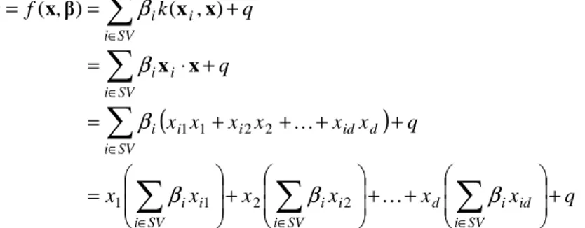
For the linear kernel example it is possible to derive an analytical expression for the parameters of the model, as a function of the Support Vector values and the corresponding coefficientsβ_i. More in details, the values of parameters a and b of “System A” and “System A_rec”, and of parameters a1 and a2 of “System B” can be obtained by substituting the definition of the linear kernel in the expression for the SVR estimating function:

(

)

q x x x x x x q x x x x x x q q k f y SV i id i d SV i i i SV i i i d id i i SV i i i SV i i i SV i i +         + +         +         = + + + + = + ⋅ = + = =

∑

∑

∑

∑

∑

∑

∈ ∈ ∈ ∈ ∈ ∈ β β β β β β K K 2 2 1 1 2 2 1 1 ) , ( ) , ( ˆ x x x x β x

where d is the length of the feature vector x, and x1,...,xd represent the single feature values. Thus, for “System A” 8

=

d and x₁=u(t−1),x₂ =u(t−2),K,x₈ =u(t−8); for “System A_rec” d=2and x₁=u(t−1),x₂ = y(t−1); for “System B” d =2and x₁=u(t−1),x₂ =u(t−2).

As a result of the SVR training phase, the set of Support Vectors xi, the corresponding βicoefficients, and the bias term q are obtained. Based on this information, the values of the model parameters can be easily computed as in the equation

above. Tables 7-9 report the obtained values compared with the true model parameters in the three examples, for different training set sizes.

Training set size a1 = 1 a2 = 0.5 a3 = 0.52 a4 = 0.53 a5 = 0.54 a6 = 0.55 a7 = 0.56 a8 = 0.57 q = 0

N=1024 0.9802 0.5780 0.1465 0.1264 0.1899 -0.0774 0.0197 0.0355 -1.01·10-5 N=100 1.0027 0.4999 0.2379 0.1319 0.0739 0.0351 -0.0204 0.0375 -8.38·10-5 N=50 1.0107 0.4770 0.2602 0.1303 0.0657 0.0349 -0.0146 0.0360 -2.14·10-4 N=10 0.9950 0.4968 0.2478 0.1206 0.0577 0.0280 0.0127 0.0027 3.23·10-3 Table 7. “System A” with linear kernel: values of the model parameters obtained for different training set sizes.

Training set size a= 1 b= 0.5 q = 0

N=1024 0.9993 0.5003 -9.89·10-6 N=100 0.9992 0.5003 2.63·10-4 N=50 0.9990 0.5001 -2.54·10-4 N=10 0.9991 0.5004 2.15·10-4

Table 8. “System A_rec” with linear kernel: values of the model parameters obtained for different training set sizes.

Training set size a1 = 1 a2 = 0.5 q = 0

N=1024 0.9991 0.5005 6.40·10-5 N=100 0.9993 0.5004 1.14·10-4 N=50 0.9989 0.5009 -3.27·10-4 N=10 0.9990 0.5004 2.11·10-4

Table 9. “System B” with linear kernel: values of the model parameters obtained for different training set sizes. Once again, we can see that for “System A_rec” and “System B”, two features are sufficient to estimate correctly all the parameters of the model (with very good approximation), even when the number of samples used for training the SVR is reduced to 10. For “System A”, a reasonable estimation is given for the first parameters, while, for parameters with true values around 10-2 it is more difficult to obtain an accurate approximation, especially for N=1024(higher number of Support Vectors). A possible reason for this is that, while two parameters (the bias term is equal to 0) are sufficient to characterize “System A_rec” and “System B”, parameters a1,...,a8 do not give a complete description of “System A” (additional term 0.5dy(t−d−1)should also be included), and need therefore to be adjusted a little with respect to their theoretical value, in order to reconstruct the true relationship between u(t) and y(t).

D. Linear kernel case: frequency domain plots

In order to have an idea of the behavior of the SVR approach also in the frequency domain, some plots are shown that depict the trend of the error of the SVR estimate.

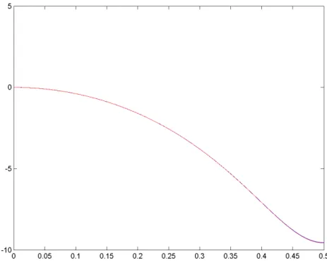
Figure 1 shows that the two frequency response functions (true model and SVR estimate) are perfectly overlapped.

Figure 1. “System B”: normalized frequency response function of the system (blue) versus the normalized frequency response function reconstructed by means of the SVR estimate with linear kernel (red).

Moreover, the amplitude in dB of the normalized error of the SVR frequency response function (with respect to the true frequency response of the system) is shown as a function of the (normalized) frequency:

dB SVR dB SVR G k U k Y k G G k G k G ) 0 ( ) ( ) ( ) ( ) 0 ( ) ( ) ( 0 0 0 0 − = −

where U(k) represents the FFT values of the test input data, and YSVR(k) is the FFT value of the SVR estimate of the output.

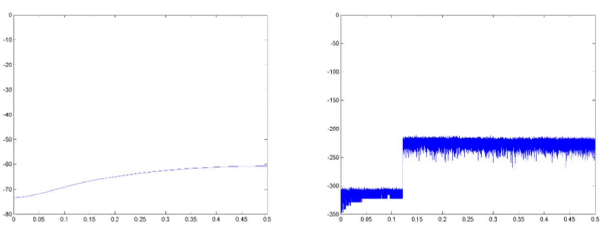
The plots are shown in Figures 2-4 for “System B” with the linear kernel function, for three different excitation signals, namely multisines with excited frequencies up to 0.12, 0.27 and 0.5. Similar figures can be obtained also for the two other cases, “System A” and “System A_rec”.

As a reference, the deviation of the frequency response function of the test data from the true model is also provided:

dB test dB test G k U k Y k G G k G k G ) 0 ( ) ( ) ( ) ( ) 0 ( ) ( ) ( 0 0 0 0 − = −

Although the latter will be obviously equal to 0 (below –300 dB in the figures), since the test data are generated starting from the true model, it is interesting to observe the different behavior in those ranges where frequencies are not excited. Multisines with excited frequencies up to 0.12 and 0.27 will not give any information for frequency values outside these ranges, resulting in a bigger error.

As far as the SVR estimate plots are concerned, no differences are observed when changing the frequency range of the excitation signal: the behavior of the system is very well reconstructed in all cases (values around –70 dB correspond to the RMSE results shown above).

Figure 2. “System B” with linear kernel, test data with excited frequencies up to 0.12: normalized error plot (amplitude in dB) in the frequency domain of the SVR estimate (left) and of the test data (right).

Figure 3. “System B” with linear kernel, test data with excited frequencies up to 0.27: normalized error plot (amplitude in dB) in the frequency domain of the SVR estimate (left) and of the test data (right).

Figure 4. “System B” with linear kernel, test data with excited frequencies up to 0.5: normalized error plot (amplitude in dB) in the frequency domain of the SVR estimate (left) and of the test data (right).

VI. Conclusions

In this work we have analysed the identification of several examples of linear systems by means of SVRs, using both non-recursive and recursive models. Different kernel functions were employed in order to better characterise the linear input-output relationship. The obtained SVR models have been used also for estimating directly the parameters of the linear system, in the case of the linear kernel. The approach based on SVR was successfully applied to all the considered examples, and frequency domain plots show that the SVR estimate approximates very well the behavior of the true system. Future directions for our reasearch will be to extend the work to the nonlinear case, and to study the effect of introducing noise on the data.

References

[1] V. Vapnik, Statistical Learning Theory, Wiley, 1998.

[2] A. Marconato, A. Boni, B. Caprile, D. Petri, “Model selection for power efficient analysis of measurement data”,

Instrumentation and Measurement Technology Conference, Sorrento, Italy, 2006.

[3] R. Pintelon, J. Schoukens, System Identification. A Frequency Domain Approach, IEEE Press, New Jersey, 2001. [4] B. Schölkopf and A. Smola, Learning with kernels, The MIT Press, 2002.

[5] O. Chapelle, V. Vapnik, O. Bousquet, S. Mukherjee, “Choosing multiple parameters for support vector machines”,

Machine Learning, vol. 46, no.1-3, pp. 131-159, 2002.

[6] B. Schölkopf, “The kernel trick for distances”, Advances in Neural Information Processing Systems, vol. 12, pp. 301-307, 2000.

[7] F. Fleuret and H. Sahbi, “Scale-invariance of support vector machines based on the triangular kernel”, 3rd

International Workshop on Statistical and Computational Theories of Vision, 2003.

[8] M.G. Genton, “Classes of kernels for machine learning: a statistics perspective”, Journal of Machine Learning

Research, vol. 2, pp. 299-312, 2001.

[9] C.-C. Chang and C.-J. Lin, LIBSVM: a library for support vector machines. Available at: http://www.csie.ntu.edu.tw/~cjlin/libsvm/