A LATENT CURVE ANALYSIS OF UNOBSERVED HETEROGENEITY IN UNIVERSITY ACHIEVEMENTS
S. Bianconcini, S. Cagnone, S. Mignani, P. Monari
1. INTRODUCTION
The evaluation of formative processes has received a growing attention by pol-icy makers and public agents with the beginning of the Bologna process, in view of identifying critical factors for achievement that can improve curricula, instruc-tional strategies, and conditions for learning. However, only recently, under a strong University internal pressure, the efficacy of a formation model integrated into students life is reassuming a central role.
A very important emerging problem is the comparison between student per-formances when different supporting and tutoring actions are adopted during the course of studies, and also in presence of very different personal situations. In order to pursue these objectives, several statistical methodologies have been de-veloped to compare student careers over time.
Given the multitude of aspects to be considered, the evaluation of formative processes may use both quantitative and qualitative methods. The complexity of the phenomenon under investigation is related to several factors, such as (a) the non experimental nature of the problem, with associated selection bias and pres-ence of confounding elements; (b) the hierarchical structure of the data, with cor-relation problems, different effects at several levels of the hierarchy and their in-teraction; (c) the multivariate and qualitative nature of the responses.
The availability of individual data repeated over a period of time allows dy-namical studies of social processes, rather than static cross-sectional analyses. In educational studies we generally deal with “micropanels”, that consists of large cross-sections of individuals observed for short time periods. They are often used to answer questions about educational progress and obstacles to such progress, mainly concerning: (a) within-individual change - How does each individual perform over time? - and (b) interindividual differences in change - What predicts differences among individuals in their change? The analysis of repeated measures has been considered from different points of view, such as individual growth techniques (Rogosa and Willett, 1985; Singer and Willett, 2004), repeated measure MANOVA and ANOVA models (Kirk, 1982), time series and econometric
analysis (Anderson, 1963; Diggle et al., 1994; Skinner and Homes, 1999; Feder et
al., 2000; Wooldridge, 2000; Arellano, 2003), and multilevel modeling (Goldstein,
2003; Srondal and Rabe-Heskett, 2004; Bryk and Raudenbush, 1989). They can be encompassed into the general class of random coefficient models, in which random effects are incorporated into the model in view of reflecting unobserved hetero-geneity in individual behavior.
When units are clustered, shared unobserved heterogeneity may induce “intra-cluster” dependence among the responses, even after conditioning on observed covariates, that can lead to incorrect inferences if not properly accounted for. This phenomenon is common for longitudinal or panel data, where observations for the same unit are influenced by the same (shared) unit-specific unobserved heterogeneity. As pointed out by Lewbel (2006), the responses can be expressed as function of the observed covariates via a structural model, that may include fixed parameters and random effects. More generally, the random coefficients can be incorporated into Structural Equation Models (SEM) by considering them as latent variables (see e.g. Bollen and Curran, 2006). As shown by Muthén et al (1987), these enable to capitalize on all the strengths of SEM, such as the use of maximum likelihood techniques for missing data, the estimation of a variety of nonlinear trajectories, measures of model fit and diagnostics to determine the source of ill-fit, the inclusion of latent covariates and repeated variable, and so on. Borrowing from Meredith and Tisak (1990), we refer to these models as Latent Curves (LCMs), since random cofficients permit each case in the sample to have a different trajectory over time. The aim of the present paper is to study growth curve models for the comparison of University student careers over time. The study has two objectives: i) evaluating the performance of groups of students dis-tinct because of the different time employed to reach the first degree, ii) evaluat-ing the effect of some covariates on the student performance. We focus on con-tinuous response variables, using conventional, normal-theory estimators, such as maximum likelihood, into the framework of SEM. The article is structured as fol-lows. First, in Section 2, the growth modeling is introduced, starting from a rela-tively simple situation and making the model increasingly complex. Then in Sec-tion 3, we apply latent curve models to a cohort of students enrolled in 2001 at the Faculty of Economics of the University of Bologna. Finally, Section 4 gives the conclusions.
2. THE MODEL 2.1 Latent curves
The basic idea behind latent curve models is that individuals differ in their growth over time, and they are likely to have different temporal behaviors as a function of differences in particular characteristics, such as gender, high school background, and so on. The approach posits the existence of continuous underly-ing or latent curves, that are not directly observed but only indirectly usunderly-ing re-peated measures.
The growth model is specified by a polynomial equation as follows
0 1 p 1, , 1, ,
it i i t ip t it
y =β +β λ +…+β λ +ε i= … n t= … T (1)
where yit is the value of the response variable y for the individual i at time point t, and β βi0, i1, ,… βip are subject-specific random coefficients assumed to be un-correlated among individuals, that is cov( ,β βij kj) 0= for every i k≠ . The argu-ment λt is a parameter that allows for the inclusion of linear or non linear trajec-tories, if the λt's are fixed or freely estimated respectively. In this latter case, a common coding convention is to have λ1 = 0 and ¸λT = 1 (McArdle, 1988). The remaining λt's reflect the proportion of change between two time points relative to the total change occurring from the first to the last period. Specifically, each value represents the cumulative proportion of total change that has occurred from the initial time to that specific point. The disturbances εit are normally dis-tributed with zero means and non constant variances. They are also uncorrelated over time (cov(ε εit, it s+ ) 0= for s ≠ ), over individuals (0 cov(ε εit, kt s+ ) 0= for
i k≠ and all s), and with the random coefficients ( cov( , ) 0β εij it = ,ji∀ ).
Key modeling results are estimates of the overall means, that are measures of central tendencies in the trajectories, and the estimates of the variation across in-dividuals of the random coefficients, as follows
ij
ij i β
β =β +ς (2)
where the disturbances ςβij ’s are assumed to be normally distributed with zero means, variances 2
ij
β
ϕ , covariances ϕβ βik, ij , and uncorrelated with the εit.
Eq. (2) can be incorporated into eq. (1) to obtain the following reduced form for the model
0 1
0 1
[ p] [ i i pi p]
it t p t t t it
y = β +β λ +…+β λ + ςβ +ς λβ + +… ς λβ +ε (3)
This shows the trajectory of y as a function of mean coefficients and a complex
disturbance term, that is heteroscedastic over time due to the presence of
, 1, ,
ij j
t j p
β
ς λ = … , whose variance depends on λt.
This model is commonly referred to as an unconditional trajectory model in which
the first term in parentheses is referred to as the fixed component, representing the mean structure of the model, and the second term is called the random part which expresses various sources of individual variability. To partially reduce such variability a conditional model can be estimated by incorporating in eq. (2) co-variates in view of testing potential influences on the trajectory parameters, as fol-lows
' , 0,1, , 1, 2, ,
j j
ij j β wi β j p i n
β =β +γ +ς = … = … (4)
where γ ’s are the regression coefficients of the time-invariant covariates w in i
the random coefficient equation, and βj are mean coefficients when the covari-ates are zero. Still ϕβij are disturbances with zero mean and variance ϕβ2ij , but
they are no longer variances of the random coefficients as in the unconditional model, since they are conditional variances.
Growth curve analysis is particularly useful when one attempts to explain the individual variation in initial status and growth parameters using background vari-ables for the individuals. These varivari-ables are viewed as causes of growth preced-ing the testpreced-ing occasion and do not vary across time. They are of substantive in-terest in that they are predictors of the growth.
Although many questions about the trajectories are possible, three are the main ones relative to (1) the characteristics of the mean trajectory of the entire group, represented by the fixed-effects components of the model; (2) the evaluation of
indi-vidual differences in trajectories, caught by the variances introduced to estimate the sampling fluctuations of the mean trajectory, and referred to be the random-effects components; (3) the potential incorporation of predictors to better understand
the variability observed in individual trajectories. As pointed out by Arellano (2003), fixed and random effects result from two different types of motivations. Fixed effects are related to the desire of exploiting panel data for controlling un-observed time-invariant heterogeneity in cross-sectional models; whereas random effects enable the use of panel data as a way of disentangling components of vari-ance and estimating transition probabilities among states, or more generally to study the dynamics of cross-sectional populations.
2.2 A structural equation perspective
Random coefficient models can be treated within the structural equation mod-eling (SEM) perspective, where the case-specific parameters that determine the trajectories are treated as latent variables. They are commonly knows as LCM. Baker (1954) was the first to suggest the use of factor analysis to study panel data. Tucker (1958) and Rao (1958) gave a more technical expression of this idea for exploratory factor analysis. Meredith and Tisak (1990) took this to the confirma-tory factor analysis and demonstrated that trajecconfirma-tory modeling fit naturally into these type of models. A number of authors expanded on this framework, among others MacArdle (1988), Browne and Du Tuot (1991) and Muthén and Khoo (1998).
Let the repeated measures yit be stacked in the vector y and the latent variables ij
β 's be stacked in η, the model can be expressed as follows =Λη ε+
y (5)
= + + +
In eq. (5), Λ is a matrix of factor loadings, and ε is the vector of time varying i errors, assumed to have zero mean and covariance matrix Θ. In eq. (6) B is a null matrix, which represent the population average parameters of the score trajectory, whereas Γ contains the regression coefficients related to the covariates w. The latent residual vector is assumed to be normally distributed with zero mean and covariance matrix Ψ=Cov( )ς .
Eq. (6) can be substituted into eq. (5) to give the reduced-form expression of y,
=Λ τ Γ+ +Λς ε+
y ( w) (7)
Differently from the classical structural equation modeling approach where the loadings are estimated, generally the LCM fixes them to specific a priori values. Moreover in SEM, the means of the factors and observed variables are usually omitted; in contrast, the LCM explicitly models both the mean and the covariance structures among the observed measures. However, a restrictive structure is im-posed on these means. Specifically, the intercepts of the repeated measures are set to zero, and the means for the latent trajectory factors are estimated. In this way the mean structure of the repeated measures is determined entirely by the means of the latent trajectory factors.
2.3 Estimation
As in the classical SEM approach model estimation is obtained by minimizing a fitting function depending on the discrepancy between the theoretical covari-ance matrix of the observed variables, Σ, and the corresponding sample covari-ance matrix, S. Hence, the information coming from the data is considered to be sufficient to get a unique estimation value of the parameters, that is, the model is identified (Bollen, 1989). However, differently from a classical SEM estimation procedure, in this case the inclusion of the information coming from the mean structure µ is also required.
Specifically from (5) and (6) we define µ and Σ as
= + µ Λ τ Γ( w) (8) + + ⎡ ⎤ = ⎢ ⎥ ⎣ ⎦ ww ε ww ww ww Λ Γ Γ Ψ Λ Θ Λ Σ Γ Λ ( S ' ) ' ΓS S ' ' S (9)
where w is the sample mean vector of the covariates and S the correspond-ww ing covariance matrix. Different fitting functions can be chosen according to the nature of the vector y. If either it is multivariate normally distributed or its com-ponents do not present excessive kurtotis the following Maximum Likelihood fit-ting function can be used (Muthén and Khoo, 1998)
1 1
ln ln ( ) ( )' ( )
ML
F = Σ − S +tr Σ−S − −p y−µ Σ− y−µ (10)
Under some regularity conditions, FML has desirable asymptotic properties as it gives asymptotically efficient estimators of the parameters and associated unbi-ased test statistics. For evaluating the goodness of fit of the SEM models the most used statistic is defined as (n-1)FML. It is asymptotically distributed as a chi-square with degrees of freedom equal to the number of the variances and covari-ances in Σ minus the number of the estimated parameters.
3. APPLICATION
With the beginning of the Bologna Process, several Universities have revalu-ated the role of the “in itinere” guidance, looking at the efficacy of a formation model integrated into the student life.
Motivated from these new requirements of the University system, we propose a first longitudinal study of students career by analyzing a cohort of students en-rolled in 2001 at the Faculty of Economics of the University of Bologna.
The study has two objectives: i) evaluating the performance of three groups of students distinct according to the different time employed to reach the first de-gree, ii) evaluating the effect of the covariates “gender” and “high school di-ploma” on the student performance.
3.1 The data
The data set analyzed was extracted from the datawarehouse of the University of Bologna. It is composed of a cohort of n=714 students. Five different time points (academic years) are observed: t1=2001/2002; t2=2002/2003; t3=2003/2004; t4=2004/2005; t5=2005/2006. Within the cohort it is possible to distinguish three different patterns:
(1) Students (n1 = 195) who got the first degree in t3 (GRAD1). (2) Students (n2 = 268) who got the first degree in t4 (GRAD2). (3) Students (n3 = 251) who did not get the degree yet (NOGRAD).
Only the first group completes the course of the study in time. The informa-tion available per each student is quite rich, allowing to build the overall student's career. In the construction of an indicator of the student performance we decided to involve the two most relevant variables, that is the mark (ranging from 18 to 30 cum laude) and the number of credits associated to each exam (ranging from 2 to 15). In detail the response variable yit is computed as the weighted average mark obtained by each student i (i = 1; 2; ... 714) over time tl (l = 1, 2, 3, 4, 5) and divided by the total number of credits required to get the degree, equal to 160. The weights are given by the credits corresponding to each exam. Thus, the vari-able obtained is continuous and it can range from 0, if the student does not pass any exam, to a maximum that depends on both the number of credits expected in each academic year and on the average of the marks.
In Table 1 and Table 2 the means, the standard deviations and the correlation matrices of the response variable across time are reported for each pattern. We can observe that GRAD1 is the group of students that presents the best average performance. It increases almost linearly during the three years. The performance of the students belonging to GRAD2 is quite good in the first three years and de-creases suddenly in the last year. It may be due to the fact that students prefer to conclude their course of study in the year t4 despite the mark obtained. The group of Nograd shows a low average performance in all the time points observed. As for the correlation values they are quite low for all the groups indicating that in general there are no strong associations between lagged performance indicators. Only in GRAD2y4 presents high negative correlations with y1, y2 and y3. It con-firms the different behaviour of this group of students in t4.
TABLE 1
Descriptive statistics for GRAD1, GRAD2, NOGRAD
GRAD1 GRAD2 NOGRAD
Mean StDev Mean StDev Mean StDev
y1 7.62 1.49 5.77 1.86 3.87 1.70 y2 8.51 1.67 6.35 1.76 4.53 1.85 y3 9.81 1.63 7.61 2.00 4.31 1.98 y4 - 4.51 2.47 4.14 2.16 y5 - - 3.05 2.83 TABLE 2 Correlation matrices
GRAD1 GRAD2 NOGRAD
y1 1.00 1.00 1.00
y2 -0.07 1.00 -0.11 1.00 0.25 1.00
y3 -0.31 -0.48 1.00 0.02 0.14 1.00 0.15 0.23 1.00
y4 - - - 0.44 0.33 0.54 1.00 -0.02 0.21 0.10 1.00
y5 - - - 0.01 -0.14 -0.02 -0.05 1.00
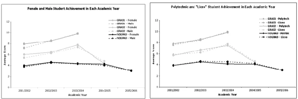
As mentioned before, the effect of two time-invariant dummy covariates, “gender” (w1, with 0=“female”, 1=“male”) and “type of diploma” (w2, with 0=“polytechnic”, 1=“high school or Liceo”), is also evaluated. As suggested in lit-erature, the former can discriminate the time pattern of the individuals, whereas the latter can provide information about the background of each student. Figure 1 shows the means of the response variable for w1 and w2 in the observed time points for each group of study.
We can notice that if the tendency of the mean performances of each pattern is analogous to the one described before for the correspondent overall pattern, it does not seem to arise either gender or type of diploma noticeable differences. However a more deep analysis within the unconditional and conditional LCM approach allows to confirm or disconfirm these preliminary results.
Figure 1 – Student performance for gender (w1) and type of diploma (w2).
4. RESULTS
Before fitting latent curve models to the data it is convenient to evaluate if GRAD1, GRAD2 and NOGRAD can be considered as three samples of the same population. Indeed since the three groups have three time points in common we can test if any difference in these observed points can be disregarded. At this aim, the data not observed for GRAD1 and GRAD2 are considered missing by design. Hence a missing data three group analysis can be conducted by assuming that the three groups have been drawn from a single population. Equality constraints are imposed for mean vector and covariance matrix elements that the three cohorts have in common. However, we rejected such an hypothesis for our data and hence the three patterns cannot be considered random samples from the same population. This requires a different latent growth specification for each of the three cohorts (Latent curve analysis is implemented by using Mplus 4.1).
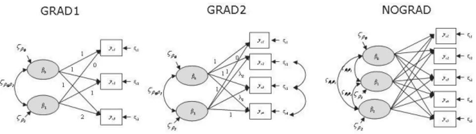
As for the students who got the degree at t1, only three time points are avail-able. It follows that only a linear growth model with uncorrelated residuals among the achievement scores is identified. In the left panel of Figure 1 the uncondi-tional model for GRAD1 is represented.
The linear growth model (Table 3) fits well with a chi-square value with one degree of freedom equal to 1.582, and p-value equal to p=0.208.
The estimates of the intercept and the slope means, equal to 7.582 and 1.071 respectively, indicate that the initial level of the students belonging to the first group is quite high and their performance increases of 1.071 between each as-sessment period. The two values are both significant, whereas there are no sig-nificant variances for the intercept (ϕˆβ0 =0.404) and slope (ϕˆβ1 =0.014). The
negative covariance between the random coefficients (equal to -0.577) is not sig-nificant too, indicating that there is no association between the student perform-ance at the initial period and its rate of change over subsequent time points.
The linear growth model for students who got the degree at t2 does not fit well. The source of this finding should not be only sought in the covariance structure, but also in the mean structure.
TABLE 3
Parameter estimation for the unconditional models, GRAD1, GRAD2, NOGRAD
GRAD1 GRAD2 NOGRAD
Estimate SE Estimate SE Estimate SE
λ1 - - - λ2 - - 0.499 0.189 - - λ3 - - 1.423 0.304 - - λ4 - - - - - λ5 - - - - - Mean β0i 7.582 0.103 5.767 0.114 3.887 0.105 β1i 1.071 0.088 -1.277 0.221 0.795 0.128 β2i - - - - -0.250 0.032 Variance β0i 0.404* 0.466 1.036 0.158 1.378 0.516 β1i 0.014* 0.243 0.293* 0.794 1.281 0.549 β2i - - - - 0.078 0.030 Covariances β0iβ1i, -0.577* 0.305 -0.866 0.220 -0.630* 0.485 β0iβ2, - - - - 0.070* 0.098 β1i,β2 - - - - -0.302 0.122 χ2 1.582 2.206 11.764 df 1 1 1 p-value 0.208 0.138 0.067 * not significant
This lack of fit suggests that linear growth is not realistic, so we explored nonlinear trajectories. We only fixed λ1= and 0 λ4= , while all others are freely 1 estimated, as represented in the central path diagram of Figure 2. By correlating the residuals between t2 and t3, and t3 and t4, the model fit results excellent (Table 3), according to the chi-square statistic [Chi-squared: 2.206, df: 1, p-value: 0.138]. The values of the freely estimated loadings are λ2= −0.499, λ3= −1.423, reveal-ing the nonlinear pattern observed in the means. There is also a significant aver-age of both the intercept (β0 =5.767) and slope β1= −1.277 factors, as well as significant variance for the intercept (ϕˆβ0 =1.036), but not for the slope
1
ˆ
(ϕβ =0.2930).
These variance components reflect that there are individual differences in the starting point, but not in the nonlinear rate of change over time. On the other hand, there is a significant negative covariance between the random intercept and slope (-0.866). Although a linear interpretation cannot be given to these results, the value of the intercept indicates that the initial level of the analyzed cohort is quite good whereas the negative slope estimate as well as the negative loading es-timates imply a decreasing growth in its performance over time and a steep in-crease at the end of the studies.
For the students who did not get the degree in the last occasion, we have observed the score for five time points. Also in this case, a linear growth model fits the data poorly, whereas a quadratic trend with uncorrelated residuals is the right one for the data of this group of student (path diagram on the right, Figure 2). This is confirmed by the chi-square value (Table 3) corresponding to a quad-ratic linear trend with six degrees of freedom equal to 11.764 (p = 0.067). All
the mean estimated result significant (3.887, 0.795, and -0.250 for β0i, β1i, and β2i, respectively). The variance estimates are all significant (ϕˆβ0i =1.378),
1
ˆ
(ϕβi =1.281), (ϕˆβ2i =0.078) as the covariance between β1i and β2i, equal to
-0.302.
Thus the students belonging to this cohort present a low initial level and, al-though the value β1i indicates on average a positive linear growth, the negative value of β2i highlights that its increment decreases with time. Considered jointly, these results reflect that the performance of this group of students is in general low since its developmental trajectory increases very slowly with magnitude of changing decelerating over time.
Figure 2 – Latent curve models for GRAD1, GRAD2and NOGRAD students.
The inclusion of covariates in the analysis allows to give further explanation of the individual variation in the initial status and growth rates. The aim of this study is to evaluate if the time-invariant covariates, gender and type of diploma, might influence the trajectory of students performance. With this regard, the conditional models described in Section 2 are applied, maintaining the growth models found in the previous analysis for all the patterns considered.
In Table 4 the parameter estimates of the conditional models for the three co-horts are reported. The chi-square tests indicate that the fitted model are good for all the three curves. We can also observe that the main parameter estimates are about the same as the ones obtained in the unconditional models. However, if we look at the regression coefficient estimates, only gender significantly predicts the intercept factor and the slope factor and only in GRAD1. That is, in the cohort of GRAD1 males (n=88) have a worse performance ( 0.647
i gen
γ = − ) than females (n=107) at the initial level but they present a positive significant slope (γgeni =0.421) indicating an improvement over time.
These differences are not present in GRAD2 and NOGRAD as the type of di-ploma do not discriminate among individuals within the three groups.
TABLE 4
Parameter estimation for the conditional models, GRAD1, GRAD2, NOGRAD
GRAD1 GRAD2 NOGRAD
Estimate SE Estimate SE Estimate SE
λ1 - - - λ2 - - -0.470 0.180 - - λ3 - - -1.378 0.289 - - λ4 - - - λ5 - - - Mean β0i 8.771 0.435 5.888 0.186 4.201 0.458 β1i 0.161* 0.375 -1.566 0.461 0.341* 0.555 β2i - - - - -0.153* 0.139 Variance β0i 0.379 0.453 1.031 0.153 1.370 0.516 β1i 0.011 0.237 0.381* 0.856 1.256 0.547 β2i - - - - 0.076 0.030 Covariances β0iβ1i, -0.574 0.296 -0.849 0.218 -0.625* 0.484 β0iβ2, - - - - 0.069* 0.097 β1i,β2 - - - - -0.296 0.122 β0i Regression γgeni -0.647 0.201 0.031* 0.063 -0.059* 0.211 γdipi -0.153* 0.207 -0.106* 0.063 -0.142* 0.214 β0i Regression γgeni 0.421 0.174 -0.016* 0.188 0.313* 0.256 γdipi 0.183* 0.178 0.196* 0.185 -0.008* 0.260 β0i Regression γgeni - - - - -0.074* 0.064 γdipi - - - - 0.008* 0.065 χ2 3.226 13.115 12.781 df 3 5 10 p-value 0.357 0.022 0.236 * not significant 4. CONCLUSIONS
In this paper we proposed a latent growth curve analysis for evaluating the ca-reer of a cohort of students enrolled in 2001 at the University of Bologna. This represents a first longitudinal study motivated by new requirements of the Uni-versity system.
From the results of the analysis we found three different subgroups or cohorts. The first one, GRAD1, is constituted by students who get the degree in the ex-pected time, that is the third academic year. They present a high initial level of performance and their growth rates increase over time. Within this group females score significantly better than males in the initial level but the latter improve their performance over time. The type of diploma does not influence the trajectory of this group.
As for the second cohort, GRAD2, it is composed by students who get the de-gree in four academic years. This is a group characterized by a quite good initial level but a negative growth rate. Furthermore these students tend to finish their course of study with a lower average score than the previous years, probably due to the need of concluding as soon as possible. The covariates considered do not affect this group of analysis.
degree yet. The results show that these students begin their studies at a low initial level and they do not improve their performance. On the contrary, their growth rate tends to decrease over time. Also for this group the covariates do not dis-criminate among individuals. It would be useful to consider different covariates to better understand different individual situations.
From a methodological point of view, we applied linear and non linear latent growth models. We considered as the response variable an indicator built as a combination of marks and credits that has been assumed to be a proxy of student performance. It would be useful to extend this class of models to the multivariate framework. Indeed, the specification of a multivariate latent growth model allows to include different response variables, each of them contributing with a proper weight in the measure of a latent student performance.
As far as we are concerned there are no applications of multivariate latent growth models within the SEM framework. This can represent a further field of investigation from both a theoretical and an applied point of view.
Dipartimento di Scienze Statistiche SILVIABIANCONCINI
Università di Bologna SILVIACAGNONE
STEFANIAMIGNANI
PAOLAMONARI
REFERENCES
T.W. ANDERSON,(1963),The use of factor analysis in the statistical analysis of multiple time series,
Psychometrika,28, pp. 1-25.
M. ARELLANO,(2003),Panel data econometrics, Oxford University press. G.A. BAKER,(1954),Factor analysis of relative growth, Growth, 18, pp. 137-143. K.A. BOLLEN,(1989),Structural equations with latent variables, Wiley, New York.
K.A BOLLEN, P.J.CURRAN, (2006), Latent curve models: a structural equation perspective, New
York:John Wiley and Sons.
K.A. BOLLEN, J.S LONG,(1993),Testing structural equation models, Newbury Park, CA: Sage. M.W. BROWNE, S.H.C. DU TOUT,(1991),Models for learning data. In L.M. Collins and J.L. Horn
(eds.), Best methods for the analysis of change, pp. 47-68, Washington D.C.: American psychological association.
A.S. BRYK, S.W.RAUDENBUSH, (1989), Towards a more appropriate conceptualization of research on school effects: a three-level hierarchical linear model. In R.D. Bock (ed.), Multilevel analysis of
educational data (pp. 159-204), San Diego, CA: Academic press.
P.J. DIGGLE, K.Y. LIANG, S.L. ZEGER,(1994), Analysis of longitudinal data, Oxford: Clarendon press. M. FEDER, G. NATHAN, D. PFEFFERMAN,(2000),Multilevel model-ing of complex survey longitudinal
data with time varying random effects, 20, Survey methodology, vol. 26, n. 1, pp. 53-65. H. GOLDSTEIN,(2003),Multilevel statistical models (3rd edition), New York: Halstead.
R.E. KIRK,(1982),Experimental design: procedures for the behavioral sciences, 2nd ed., Monterey,
CA: Brooks/Cole.
A. LEWBEL,(2006),Modeling heterogeneity,Working paper, Boston College.
J.J. MCARDLE,(1988), Dynamic but structural equation modeling of repeated measures data. In J. R.
Nesselroade and R.B. Cattel (eds.), The handbook of multivariate experimental psychology, 2nd ed., pp. 561-614, NewYork: Plenum press.
W. MEREDITH, J. TISAK,(1990), Latent curve analysis, Psychometrika, 55, 1, pp. 107-122. R.O. MUELLER, (1996), Basic principles of structural equation modeling, Springer-Verlag, New
York.
B. MUTHÉN, D. KAPLAN, M. HOLLIS (1987),On structural equation modeling with data that are not missing completely at random. Psychometrika, 42, pp. 431-462.
B. MUTHÉN, S.T. KHOO(1998), Longitudinal Studies of Achievement Growth Using Latent Variable Modeling, Learning and Individual Differences, 10 (2), pp. 73-101.
C.R. RAO,(1958),Some statistical methods for comparison of growth curves, Biometrics, 14, pp. 1-17. D.R. ROGOSA, J.B. WILLETT,(1985),Understanding correlates of change by modeling individual differences
in growth, Psychometrika, 50, pp. 203-228.
C.J. SKINNER, D. HOLMES,(1999), Random effects models for longitudinal survey data, paper
pre-sented at the Conference on analysis of survey data, Southampton, United Kingdom.
J.D. SINGER, J.B .WILLETT,(2004),Applied longitudinal data analysis: modeling change and event occur-ence, New York: Oxford University press.
A. SKRONDAL, S. RABE-HESKET,(2004),Generalized latent variable modeling: multilevel longitudinal and structural equation models. Boca Raton, FL: Chapman and Hall/CRC.
J.M. WOOLDRIDGE,(2000),Econometric analysis of cross section and panel data, Cambridge: MIT
press.
L.R. TUCKER,(1958), Determination of parameters of a functional relation by factor analysis,
Psycho-metrika, 23, pp. 19-23.
SUMMARY
A latent curve analysis of unobserved heterogeneity in university achievements
The aim of this paper is to analyze the academic achievement of a cohort of students enrolled in 2001 at the Faculty of Economics of the University of Bologna by using a la-tent growth model for longitudinal data. The basic idea of this approach is that individuals differ in their growth over time according to a continuous underlying or latent trajectory. Random coefficients in the model allow each individual to have a different trajectory. La-tent growth models can be incorporated in the Structural Equation Models (SEMs) framework by viewing the random coefficients as latent variables. Hence model identifi-cation and estimation are performed according to the conventions of the SEM analysis. The effects of different covariates in the student temporal behavior is also evaluated.