LAT Data Analysis: the case of
EGRET pulsars
In this chapter I present a basic analysis of simulated γ-ray pulsars as observed by LAT. This Chapter has two main goals: first of all to show what are the main analysis tools and techniques developed by the LAT collaboration for LAT data analysis. Second, in this Chapter it is shown how the PulsarSpectrum simulator can be used to produce simulated dataset that can be useful for testing analysis tools. In this sense some analysis case will be presented, together with examples of how analysis tools can be used and what analysis scripts and techniques I developed as a part of my Ph.D. for managing some simple data analysis of pulsars with the LAT.
The analysis cases presented are based on simulation of 30 days of LAT obsevation in scanning mode.
A typical analysis of a pulsar can be divided in three main categories, Spatial Analysis, Temporal Analysis and Spectral Analysis. These kind of analyses are typical for every sources, but for pulsars temporal analysis has a particular importance, since it can provide a very powerful tool for identifying a γ-ray source with a pulsar using periodic modulation of γ-rays.
The tools available for analyzing LAT data consist of a set of LAT SAE tools specific for basic pulsar analysis. After the basic data reduction a lot of different tools can be used for each kind of analysis. For the analyses carried out in this Chapter I used several analysis packages and tools, in particular the FTOOLS suite 1
for basic manipulation of FITS files, then ROOT Analysis Framework2
and a set of Python scripts developed for performing automatic analysis of large set of pulsars, as it will be described in next Chapters.
Some specific analysis have been chosen here, in particular a basic temporal analysis of Vela pulsar, in order to show how the periodicity can be easily tested for a bright source. Then the case of PSR B1706-44 is considered, as an example of standard analysis chain consisting of spatial, spectral and temporal analysis. Then an analysis of simulated pulsar PSR B1951+32 show how a fainter pulsar can be analyzed. These analyses are very basic and can be expanded in several ways, as for example the study the phase-resolved spectroscopy in case of pulsars that give enough counts.
1
Seehttp : //heasarc.gsf c.nasa.gov/f tools/f toolsmenu.html 2
Seehttp : //root.cern.ch/
6.1
Pulsar Data Analysis
The three basic properties that are of concern by the γ-ray pulsar studies are the spatial, temporal and spectral distribution of photons.
The γ-ray experiments like the LAT are counting telescopes and for each detected pho-ton and energy, an arrival time and a direction are reconstruct. The analysis is done by looking at the distribution of these three variables to derive the characteristics of the source.
Although this is true for all energies, the methods of analysis are as varied as the energy bands in which pulsars are observed. The primary difference between γ-ray astrophysics analysis and analysis at lower energies is the relative sparseness of the data. In order to detect sources in γ-ray observations of the order of days are required.
The better statistics and resolution available by the LAT will permit high-detailed stud-ies on point sources and in particular on pulsars.
In Ch. 2 the LAT Science Analysis Environment (SAE) has been presented. It consists of a suite of tools devoted to the data analysis of the LAT data. In particular there are some tools devoted to the data analysis of the LAT data. In particular there are some tools to perform analysis while some other provide analysis for particular source classes. As for previous experiments such as EGRET, the spatial analysis, that is done mainly using the maximum likelihood technique, is performed using the tool called gtlikelihood. The timing analysis of pulsars in the SAE includes several tools that have been described in Ch. 2.
The spectral analysis can be performed using the maximum likelihood, since this tools provides also fit with the spectrum. A second approach is to build input files that can be used with the XSpec package3
.
6.1.1
Spatial Analysis
To perform a sensitive search for point sources it is necessary to do more than look for emission above the predicted diffuse background. If an excess is truly due to a point source, it will be spatially distributed as the energy dependent PSF of the instrument. The technique used in analyzing γ-ray data in COS B and EGRET was the maximum likelihood method, fully described in (Mattox et al., 1996). This technique allow the possibility to identify a point source above the background and to estimate the total flux. I briefly review the basic concepts of the method.
Maximum Likelihood method use the Instrument Response Function, that can be writ-ten in the most general form as:
R(E′, ˆp′; E, ˆp, t) = A(E, ˆp, t)P ( ˆp′; E, ˆp, t)D(E′; E, ˆp, t) (6.1)
where E is the true photon energy, ˆp the true photon direction, E’ is the measured photon energy and ˆp′ the measured photon direction. The function A(E, ˆp, t) is the
instrument effective area, P ( ˆp′; E, ˆp, t) is the Point Spread Function and D(E′; E, ˆp, t)
is the energy dispersion.
3
EGRET used binned Poisson likelihood defined as: L(µ) =Y ij µnij ij e−µij nij! (6.2) where the sky map under analysis was binned in spatial bins (i,j). In this Equation µij
is the predicted number of counts in bin (i,j) and nij the measured number of counts
in the bin (i,j). The bin width in sky coordinated, e.g. Right Ascension or Declination, was 0.5◦. Count maps for energy above 100 MeV were used for detection, identification
and flux extimation. This method was also used for spectral analysis of EGRET data, using 10 standard energy bands from 30 MeV to 10 GeV. A single effective Point Spread Function (for a given measured energy range) was used for convolving the diffuse model and for estimating counts for each of the sources, regardless of intrinsic spectrum. The nature of the LAT response functions motivated the use of an Unbinned likelihood for some reasons. First of all the relatively broad PSF and the high number of expected sources imply that emission from nearby point sources always overlaps. The amount of overlap is less severe for photons above 1 GeV. Second, the Point Spread Function strongly depend on the energy, then the intrinsic spectrum of a source affects the degree of source confusion. Third, the large Field of View and the variation of response in function of incident angle, combined with the scanning mode makes almost impossible to compute a response function valid for all events.
The Unbinned Likelihood is the limiting case of a binned analysis with infinesimally small bins, each containing 0 or 1 count. In this method the data space considered includes an energy axis as well as photon direction. Differently from EGRET, here the spectral fitting is not decoupled from the source flux estimation.
Presently the LAT SAE contain the tool gtlikelihoof that is able to perform both Un-binned Likelihood and the Binned Likelihood analysis. In the analysis of this Chapted I will use the Unbinned Likelihood for spatial analysis of pulsars under consideration. Here then the basic of the Unbinned Likelihood is described, while the Binned Likeli-hood does not differ significantly from the EGRET likeliLikeli-hood method.
The region of the sky that is under analysis can be modeled including point sources with intensity si(E, t), the Galactic diffuse emission SG(E, ˆp) and extragalactic diffuse
emission SEG(E, ˆp) and possibly time varying sources Sl (e.g. Moon, SNRs, etc..).
The Source Model can be written as: S(E, ˆp, t) =X
i
si(E, t)δ(ˆp − ˆpi) + SG(E, ˆp) + SEG(E, ˆp) +
X
l
Sl(E, ˆp, t) (6.3)
The Region Of Interest (ROI) is the defined as the extraction region for the data in measured energy, direction and arrival time.
Give the Source Model it is possible to compute the event distribution function M, i.e. the number of expected events gived the model.
M (E′, ˆp′, t) =
Z
SR
R(E′, ˆp′; E, ˆp, t)S(E, ˆp, t)dEdˆp (6.4)
where the Source Region SR is defined as the portion of the sky that contain all sources that contribute significantly to the ROI.
The predicted number of observed events in the ROI is the integral of M over the ROI: Npred=
Z
ROI
M (E′, ˆp′, t)dE′d ˆp′dt (6.5)
This calculation can be aided gretaly by defining the quantity ǫ(E, ˆp) that is similar to the exposure map computed by EGRET:
ǫ(E, ˆp) ≡ Z
ROI
R(E, E′, ˆp, ˆp′, d)dE′d ˆp′ (6.6)
where primed quantities indicate measured energies,E′, and measured directions, ˆp′.
This type of exposure map used by unbinned Likelihood differs significantly from the EGRET exposure maps, which are integrals of effective area over time.
The number of predicted events is then: Npred=
Z
SR
ǫ(E, ˆp)S(E, ˆp)dEdˆp (6.7)
All these operations are implemented in the SAE tool with specific tools, in particular gtexpmap.
Finally, the unibinned likelihood can be computed as: log(L(µ)) =X
j
log M (E′, ˆp′, t) − N
pred (6.8)
where the sum is taken over all the events j . The quantity L(µ) is referred to as the likelihood function. Comparing this to the expression for the binned likelihood, the first term can be identified with the factor Qijµij and the second term with Qije−µij.
We call with ˆµ the optimal model parameters in Eq. 6.2, i.e. the ones that maximize L(µ), or equivalently lnL(µ).
The Binned Likelihod start from the Eq. 6.2 and compute the expected counts µij in
the (i,j)-th bin from the sum of k sources using the response function as: µij = X k X ij Z dt Z SR
R(E′, ˆp′; E, ˆp, t)Sk(E, ˆp, t)dEdˆp (6.9)
It is also possible to assume a model µ0 with no sources, i.e. the null hypothesis. In
alternative, a model with N source we call µN. The likelihood ratio λN is defined as:
λN =
L( ˆµ0)
L(ˆµN)
(6.10) As the maximum likelihood estimator ˆµ asymptotically approaches the true spatial distribution of the γ-rays, the test statistic, usually called T SN ≡ −2lnλN will be
distributed as a χ2
(N ) (Fierro, 1995; Mattox et al., 1996).
Thus, the significance S of a detection of a source at a specific position is: S = Z ∞ T SN 1 2χ 2 1(ξ)dξ = Z ∞ √ T SN e−η2 /s √ 2π dη (6.11)
Where we have used the integrand substitution η=ξ1/2
. The 1/2 factor at the first integral of Eq. 6.11 takes into account that counts number in a bin is always positive, eliminating one half of the statistical fluctuations. From Eq. 6.11 and adopting the common pratice to indicate the significance as a results of nσ, it turns out that the significance of a source is √Tsσ.
This method provide the possibility to determine the existence of a source and also gives an estimated of the counts that can be combined with the exposure to obtain the source flux. Additionally this method is very useful to provide also a spectral model of the source, allowing the user to perform a spectral analysis on the data.
6.1.2
Temporal Analysis
The problem with identifying γ-ray sources on the basis of their spatial proximity to the known positions of sources at other wavelength is the possibility of a purely coincidental position alignment. In the case of EGRET a typical likelihood contour had a radius of 0.5◦and in many cases of 3EG sources no definitive association can be established(Fierro,
1995). A definite association with a pulsar can be established by finding a γ-ray signal modulated at the period of the known radio pulsars. This method works well for radio-loud pulsars, but for radio-quiet pulsars like Geminga the signal periodicity has to be found with totally different techniques of blind periodicity search.
For this reason radio-astronomers teams will coordinate with the GLAST community in order to provide updated ephemerides for a list of candidate γ-ray pulsars.
The low fluxes of γ-ray sources require combining different observations to improve the statistics. For pulsed analyses this requires that each γ-ray detected by the pulsar must be tagged with a corresponding rotational phase, i.e. the fraction of revolution at which a γ-ray emitted from the pulsar is detected at the LAT at the measured arrival time. Once the phase assignment, of phase-tagging has ben performed, the pulse analysis (e.g. phase-resolved spectral analysis) can be done.
The temporal analysis procedure for pulsars consists of three steps. The first are the so-called barycentric corrections (See also Ch. 5), where the arrival times at the instrument, which are expressed in Terrestrial Time4
, are converted to arrival times at the Solar System Barycenter, and expressed in Barycetric Dynamical Time5
.
This procedure is performed by using the tool gtbary, parts of the LAT SAE. It requires the file that describe the position of the LAT during the simulation and the position of the celestial sources.
Once the barycentric corrections have been applied and the arrival times have been referred to Solar System barycenter, it is possible to assign a phase to each photon. The phase is assigned according to ephemerides as following Eq. 5.7.At this point the lightcurve is obtained.
It is also possible to perform some tests for priodicy of the source. The three main tests used in GLAST LAT presently are the χ2
test (Leahy et al., 1983), the Z2
n(Buccheri et al.,
1983) test and the H-test(de Jager et al., 1989). Here I will use for these examples the χ2
test for testing periodicity of lightcurve.
The basic periodicy test for photons covering a time range T is to assign phases for
4
For a definition of Terrestrial Time see Ch. 5 5
a range of trial periods from Pmin = 2T/i1 up to Pmax = 2T/i2, with i = i2,i2+1,...i1.
Thus in this case the frequency spacing is 1/2T and the period can be searched is steps of frequency resolution divided by two, but in this analysis also smaller frequency steps are used. The obtained phases are then folded in n bins. In absence of pulsations, or any secular trends, the counts in each bin of a lightcurve obtained by folding at a given period are Poisson distributed, with mean and variance best estimated by the mean number of count per bin ¯m. If the counts mi counts in each phase bin i is large enough
to assume to be normally distributed, then the statistics S: S = n X j=1 (mj − mexp)2 mexp (6.12) is a χ2
with n-1 degrees of freedom. Then it follows that the probability that the observed signal at any particular period will exceed by chance a level S0 is given by the
integrated χ2 distribution: Qn−1(χ20 = S0) = Z ∞ s0 pn−1(χ2)dχ2 (6.13) where pn−1(χ2 ) is the χ2
distribution. It is possible to relate this expression with the (percent) confidence level c, such that S0 has not been exceeded by chance given Np
periods(Leahy et al., 1983),
1 − c/100 = NpQn−1(χ 2
0 = S0) (6.14)
Another periodicity test is the Z2
n-Test(Buccheri et al., 1983), that is based on the
variable Z2 n defined as: Z2 n= 2 n X k=0 (α2 k+ β 2 k) (6.15)
where n is the number of harmonics to be considered and the α2
k and β 2
k are defined as:
αk= (1/N ) N X i=1 cos kφi (6.16) βk = (1/N ) N X i=1 sin kφi (6.17)
where N is the number of photons and the φi’s indicate the phases of each photon. It
have been shown that in the limit of infinite m the Z2
n follows a χ 2
distribution with 2n degrees of fredom.
This method is an improvement with respect to the χ2
test, but it has a big limitation, as well as the Chi squared test. Both these tests depend upon a smoothing parameter (the number of bins for χ2
and the number of harmonics for Z2
n). The power of these
tests depend critically on the lightcurve shape (de Jager et al., 2002). For example, in order to detectd a broad peak one should use small values of m or number of bins, but narrow peaks in the lightcurve are best identified when using large values of number of bins.
A great improvement is given by the H-Test, that uses the Z2
n as a basis but present a
solution to the choice of the number of harmonics. The H variable is defined as: H ≡ max1 <m<inf(Z 2 n− 4m + 4) = Z 2 M − 4M + 4 (6.18)
A detailed discussion of this test and of its power can be found in (de Jager et al., 2002). When the period is not exactly know, because of a lack of radio observation in the time range of the data, it is possible to estimate the central frequency and then check for the periodicity in order to find the value of frequency with the highest confidence level. Once this frequency is found, it is possible to assign the phases to obtain the lightcurve. In this thesis mainly the χ2
-Test and H-Test will be used, and in this Chapter examples of both will be reviewed.
6.1.3
Spectral Analysis
In addition to the total flux determined by the Likelihood analysis and the pulse profile from temporal analysis it is important to measure the energy distribution of the photons coming from the source.
Since energy dispersion and effective area vary with the incidence angle, the distribution of the measured energies do not match the true energy spectrum. It is then important to de-convolve the measured spectrum with the response function of the instrument. For spectral analysis several standard tools already exist and in this thesis I will use two different approaches that I will discuss briefly here.
The first approach uses the maximum likelihood method for estimating spectral param-eters as discussed about the spatial analysis. With this tools it is possible to give as input a source model with a parameterized differential spectrum and the likelihood tools of the SAE return the values of spectral parameters that maximize the likelihood. Addi-tionally the energy distribution of the counts from the model are also provided, usually divided in contribution of the source and of the component of the diffuse background. The second approach followed in this thesis use the standard package XSpec widely used in X-ray astronomy 6
. The approach of XSpec is based on the fact that a source spec-trum f (E) will give an observed count C(I) in a specific energy bin or energy channel I is given by:
C(I) = Z ∞
0
f (E)R(I, E)dE (6.19)
where R(I, E) is the Instrument Response Function and it is proportional to the prob-ablity that an incoming photon of energy E will be detected in energy channel I. Since LAT is a counting telescope and data can be binned in energy channels, this approach can also be used, with the caution that in general the counts are smaller than counts in a typical X-ray telescope.
Ideally we would like to determine the actual spectrum of a source, f (E), by inverting this equation, thus deriving f (E) for a given set of C(I). Unfortunately this is not pos-sible in general, as such inversions tend to be non-unique and unstable to small changes in C(I).
The alternative used by XSpec is to choose a trial model spectrum fm(E) that can be 6
described in terms of parameters pi and match to the data obtained by the instrument.
For each fm(E) a predicted count spectrum Cp(I) us computed in order to judge how
well it fit the observed counts.
The model parameters then are varied to find the parameter values that give the most desirable fit statistic. These values are referred to as the best-fit parameters. The model spectrum, fb(E), made up of the best-fit parameters is considered to be the best-fit
model.
XSpec uses the most common fit statistic for determining the best-fit model, i.e. the χ2
statistics, where the χ2
is defined is the same formula as Eq. 6.12, where now the mj
and mexp refer to observed and expected counts in the j-th energy bin instead of phase
bin.
An example of analysis using XSpec will be presented here and in Ch. 9. In order to analyze data with XSpec the LAT data must be converted in spectrum files (.PHA) and Response Matrix files (.RMF). The PHA files are files where the observed counts are binned in energy bins defined by the user and the RMF represent the response function of the instrument and are computed considering the LAT orbit and IRF. Both files can be created from the LAT SAE using the gtbin tool for creating PHA spectra and gtrsp-gen for creating response matrix RMF files.
6.2
Description of the EGRET pulsar Dataset
For these analysis I simulated one month of GLAST LAT observations in normal rocking mode. The orbital period is set 95 to minutes, with a rocking angle of 35 ◦.
For the simulation I used the program Observation Simulator, described in Ch. 2 and I have used part of the LAT SAE for the spatial and timing analysis, and some other scripts developed in Python, ROOT and IDL for plotting and doing simple analysis. The starting date of the observation has been fixed to Jan 1, 2009, corresponding to MJD 54832 7
.
The launch will take place in the second part of 2007, but for our purposes the total simulation time is more important than its start date.
The main component of the simulations have been all the γ-ray pulsars presently known, i.e Vela pulsar, Crab pulsar, Geminga, PSR B1706-44, PSR 1055-52 and PSR B1951+32. with parameters that will be described below, all of them simulated using lightcurve from EGRET data and spectra simulated using a power law with super-exponential cutoff. To these point sources I have added a simulated diffuse Galactic and extragalactic emis-sion γ-ray emisemis-sion. The Galactic emisemis-sion distribution has been derived by the EGRET γ-ray diffuse map (Figure 6.1)and the simulated spectrum is a power law with spectral index equal to 2.1 and a total flux from 10 MeV to above 655 GeV of Fgal=18.58
ph m−2s−1 in this energy range.
The extragalactic diffuse emission has been modeled as a power-law with spectral index of 2.1 and a total flux of Fextr=10.7 ph m−2s−1 between 20 MeV and 200 GeV.
7
MJD indicates the Modified Julian Date and it is related by the Julian Date by MJD = JD-24000000.5
Figure 6.1: Intensity map for the Galactic diffuse γ-ray emission used in the simulations of this Chapter. The map has been determined using GALPROP. Courtesy of Seth W. Digel, LAT Collaboration.
6.3
Testing the periodicity of a bright pulsar: the
case of Vela
Vela pulsar (PSR B0833-45) is the brightest γ-ray pulsar. The individual pulses at about 89 ms can be easily distinguished in radio observations. The age of about 11000 year has helped to identify it with the product of the supernova explosion that creates the Vela Supernova Remnant.
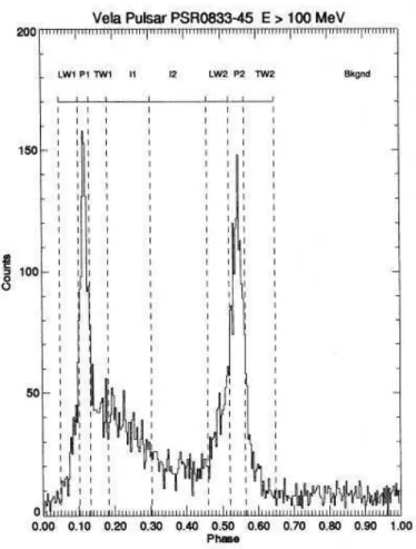
Gamma-ray emission from Vela were found in SAS-2 data and one of the first remarkably surprises was that the γ-ray lightcurve shows two peaks separated by about 0.4 in phase, while the radio lightcurve shows a single peak. EGRET has given the opportunity to study in more detail this pulsar and two complete reports can be found in (Fierro, 1995; Kanbach et al., 1994).
In this section I will outline a basic temporal analysis on Vela pulsar, describing how LAT tools can be used to test periodicity of a pulsar. The case of Vela is particularly interesting since the periodicity of the γ-rays is clearly visible.
6.3.1
Simulated Dataset
The simulation model used for Vela pulsar has been created using PulsarSpectrum and PSRPhenom model described in Ch. 5. The source has been placed at the position of the radio pulsar retrieved from the ATNF catalog at equatorial coordinates α2000=128.83588
and δ2000=-45.17635. The lightcurve is based on EGRET observation and have been
smoothed using a boxcar smoothing algorithm with window of 2 phase bins of width 0.01 in phase, in order to remove statistical fluctuations in the original lightcurve. Such a value is a compromise between a small smoothing window, that can introduce artifacts, and a larger one, that can remove also real structures in the lightcurve of the pulsar. The number of time bin in the smoothed lightcurve has been increased to 8000 by
Figure 6.2: Simulated lightcurve for PSR B0833-45. The histogram represent the original EGRET data from (Fierro, 1995) where the lightcurve is binned in 100 phase bins. The dotted blue histogram is the smoothed lightcurve using boxcar algorithm, and the solid line is the resulting lightcurve of 8000 bins using after interpolating the dotted histogram.
interpolation, in order to obtain a bin width of about 11 µs. The resulting lightcurve is displayed in Fig. 6.2. This lightcurve has been taken from (Fierro, 1995) and has been assigned phase 0 the first bin for pratical reasons, then it appear shifted with respect to the original EGRET lightcurve, where phase zero was taken to be the phase of the radio pulse.
The ephemerides have been obtained by radio ephemerides used for EGRET (Fierro, 1995) and the reference epoch was MJD 49605. The simulated dataset start at MJD 54832, then I have decided to mantain the same ephemerides and shift the reference epoch to MJD 54851. The ephemerides used for this pulsar are reported in Tab. 6.3.1:
Vela Ephemerides (Fierro, 1995)
Epoch (MJD) 54851 f (t0) (s−1) 11.197226013404 ˙ f (t0) (s−2) -1.536636×10⁻¹¹ ¨ f (t0) (s−3) 6.26×10⁻²²
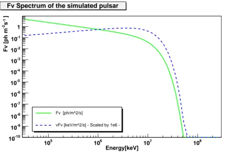
The spectrum is modeled in the basis of a power law with super exponential cutoff, with parameters retrevied from (Nel & de Jager, 1995; de Jager et al., 2002). The spectral index for the power law is g=1.62 and the cutoff energy E0 is set to 8 GeV. The cutoff is
super exponential, with a value of b=1.7. The resulting spectrum is shown in Fig. 6.3. According to the value reported by EGRET, the total flux of the pulsar has been set to (9×10⁻⁶ ph cm−2s−1).
Energy[keV] 5 10 106 107 108 ] -1 s -2 Fv [ph m -10 10 -9 10 -8 10 -7 10 -6 10 -5 10 -4 10 -3 10 -2 10 -1 10 1 Fv [ph/m^2/s]
vFv [keV/m^2/s] Scaled by 1e6
-Fv Spectrum of the simulated pulsar
Figure 6.3: Simulated spectrum of PSR B0833-45 using a power law with exponential cutoff. The flux and νFν distributions are showed
. 0 5 10 15 20 25 6:40:00.0 8:00:00.0 9:20:00.0 10:40:00.0 -59:59:59.8 -39:59:59.9 -29:59:59.9
Figure 6.4: Count map of the region within 20◦ around position of Vela pulsar in
equa-torial coordinates obtained using the LAT SAE tool gtbin. The position of the radio source is indicated by a cross.
6.3.2
Periodicity testing
The count map of Vela pulsar is displayed in Fig. 6.4 in equatorial coordinates, that comprises a region of 20◦ around the position of the source. This count map has been
obtained using a SAE tool called gtbin, and photon counts have been binned with a bin width of 0.25◦.
This pulsar corresponds to the source 3EG J0834-4511 in the Third EGRET Catalog (Hartman et al., 1999). From the skymap it is visible that Vela is a very bright source, that overwhelm the diffuse γ-ray emission.
The position used in the barycentric corrections for Vela pulsar is α2000=128.83588◦,
δ2000 = −45.17635◦. First a region of radius of 3◦ has been selected.This radius is
compatible with the Point Spread Function of the LAT. A more refined analysis should take into account that PSF radius varies with energy and thus implements an energy-dependent cut.
The periodicity test is a critical step in order to confirm that γ-rays are modulated at the same periodicity of the radio pulsar. This is a powerful tools for identifying a γ-ray source with a pulsar.
In order to do that, I use the LAT SAE tool called gtpseach, that can apply the χ2
, Z2 nand
H-Test to the data file. I used the barycentered file obtained by gtbary. Since the total observation time is of 1 month, i.e. T=2.592×10⁶
s., the correspondent Independent Frequency spacing (IFS) is 1/T≃4×10−7 Hz. Since in the periodicity test the trial
frequencies are spanned at fixed frequency steps expressed as fraction of IFS, then then I will assume as error on the frequency one half of the frequency step of the scan. The
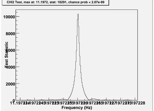
Frequency (Hz) 11.19721611.19721811.1972211.19722211.19722411.19722611.19722811.1972311.19723211.19723411.197236 Test Statistic 0 1000 2000 3000 4000 5000 6000 7000 8000
CHI2 Test, max at: 11.1972, stat: 7677.11, chance prob < 2.07e-99
Figure 6.5: χ2 applied to Vela pulsar by taking into account the frequency first deriva-tive.
starting value for the central frequency is 11.19722 Hz. This value has been chosen by approximating the radio frequency, in order to check if the periodicity search leads to the correct frequency of the signal. In order to better apply the χ2
-Test for periodicity I considered also the frequency derivatives. The frequencies are scanned at intervals
Frequency (Hz) 11.19722411.197224511.19722511.197225511.19722611.197226511.19722711.197227511.197228 Test Statistic 0 2000 4000 6000 8000 10000
CHI2 Test, max at: 11.1972, stat: 10291, chance prob < 2.07e-99
Figure 6.6: χ2 applied to Vela pulsar by taking into account the frequency first derivative and ”zooming” on the central frequency
of 0.5 IFS, i.e. 2×10⁻⁷ Hz, I assumed as error on the frequency estimate a value of
10−7 Hz. The results are very good and the peak corresponding to the frequency of the
pulsar is clearly visible in Fig. 6.5. A value of 11.1972259±(1×10⁻⁷) Hz is obtained.
This test has been performed with 200 trial frequencies centered at the approximated frequency 11.19722. The used bin number is 20. The statistics S is higher , S=7667.11, corresponding to a chance probability p<2×10−99, meaning that periodicity is very clear.
I then refined this value by a ”zoom” in frequency around the central peak, by choosing steps of 0.05 the frequency resolution centered on the previous value. The frequencies are scanned at intervals of 0.5 IFS, i.e. 2×10⁻⁸ Hz, I assumed as error on the frequency
estimate a value of 10−8 Hz.The result is remarkably better and the obtained frequency
is displayed in Fig. 6.6. A value of 11.19722601±(2×10⁻⁸) Hz is obtained. This test
has been performed with 200 trial frequencies centered at the frequency found with the previous test. The used bin number is 20. The statistics S is higher , S=10290.2, corresponding to a chance probability p< 2 ×10−99. This means that the periodicy have
been found with very high confidence level. In particular the found frequency agree within the error with the simulated frequency at epoch. At this point the identification with the Vela Pulsar could be confirmed.
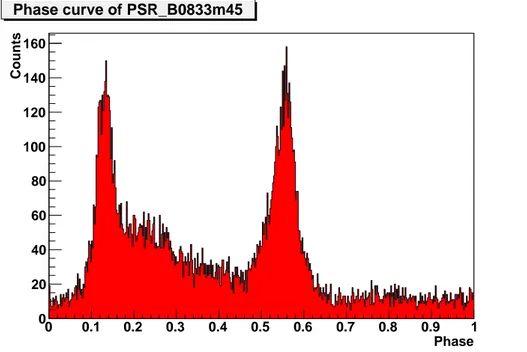
Once the periodicity has been confirmed, to each photon a rotational phase can be assigned using the Eq. 5.7 in Ch. 5 in order to obtain the reconstructed lightcurve. The photons arrival times have been phase-assigned in order to obtain the lightcurve, displayed in Fig. 6.7.
The TimeProfile used for this simulated has been obtained from EGRET observation (Fierro, 1995), then by comparing the reconstructed lightcurve with the Vela pulsar seen
Phase 0 0.1 0.2 0.3 0.4 0.5 0.6 0.7 0.8 0.9 1 Counts 0 20 40 60 80 100 120 140 160 Phase curve of PSR_B0833m45
Figure 6.7: Reconstructed lightcurve using 450 bins of Vela Pulsar after the steps de-scribed in text for periodicity test.
by EGRET, e.g. in (Kanbach et al., 1994) (Fig. 6.8), it is possible to see that they are very similar.
This is the expected result and confirms that all calculations and timing corrections in the simulation have been performed correctly by PulsarSpectrum.
6.4
The analysis of PSR B1706-44
The γ-ray emission from PSR B1706-44 was discovered by EGRET (Thompson et al., 1992). The 102 ms radio pulsar was discovered during a radio survey of the southern Galactic plane and this pulsar was coincident with the COS B source 2CG 342-02 (Fierro, 1995).
The unpulsed X-ray emission has ben discovered in 1995 by ROSAT and then the pulsations have been detected using Chandra telescope in 2002 (Gotthelf et al., 2002). The low statistics of COS B did not allow the discovery of this γ-ray pulsar, but the EGRET observations revealed pulsed γ-ray emission from this source.
Unlike the first three pulsar detected (Vela, Crab and Geminga), PSR B1706-44 shows a different pulse profile, consisting in a single broad peak spanning about 35% of the total period. Since this pulsar is much more weak than Vela, it is more difficult to resolve the lightcurve in detail. PSR B1706 shows a young age τc ∼ 1.7 × 10⁴years and a there are
some Supernova Remnants candidates for association with this pulsar (Fierro, 1995). Using radio data and a distance of 2.4 kpc the total rotational energy loss is about
˙
E = 3.4 × 1036
erg s−1. The γ-ray luminosity measured by EGRET is of about L ≈
5 ×1034
× 4πf erg s−1, where f is the beaming fraction in steradian. Unless the beaming fraction is extremely small, the γ-ray radiation represent about the 1% of the total
Figure 6.8: The EGRET lightcurve of Vela pulsar obtained by Kanbach et al. in (Kan-bach et al., 1994)
rotational energy loss.
6.4.1
Simulation of PSR B1706-44
The simulation model used for PSR B1706-44 has been created with PulsarSpectrum and PSRPhenom model described in Ch. 5. The source has been placed at the po-sition of the radio pulsar retrieved from the ATNF catalog at equatorial coordinates α2000=257.42403◦ and δ2000=-44.48562◦. The lightcurve is based on EGRET
observa-tion and have been smoothed using a boxcar smoothing algorithm with window of 2 phase bins, in order to remove statistical fluctuations in the original lightcurve. As the case of Vela pulsar, this appear to be a good compromise to reduce statistical fluctua-tions and mantain lightcurve structure. The period of 102 ms and the goal to have a small bin width (∼ 10µs, smaller than LAT dead time), lead to a large number of 10000 bins, obtained by interpolating the smoothed lightcurve. This results in a bin width of about 10 µs. The resulting lightcurve is displayed in Fig. 6.9. The original epoch for the epherides was MJD 49447 (Fierro, 1995), but it has been shifted to MJD 54847, because it is nearer the start date of the simulation, MJD 54832. The radio ephemerides used for the phase assignment are the following:
Figure 6.9: Simulated lightcurve for PSR B1706-44. The histogram represent the orig-inal EGRET data from (Fierro, 1995) where the lightcurve is binned in 50 phase bins. The dotted blue histogram is the smoothed lightcurve using boxcar algorithm, and the solid line is the resulting lightcurve of 10000 bins using after interpolating the dotted histogram. Energy[keV] 5 10 106 107 108 ] -1 s -2 Fv [ph m -10 10 -9 10 -8 10 -7 10 -6 10 -5 10 -4 10 -3 10 -2 10 -1 10 1 Fv [ph/m^2/s]
vFv [keV/m^2/s] Scaled by 1e6
-Fv Spectrum of the simulated pulsar
Figure 6.10: Simulated spectrum of PSR B1706-44 using a power law with exponential cutoff. The flux and νFν distributions are showed
. PSR B1706-44 Ephemerides (Fierro, 1995) Epoch (MJD) 54847 f (t0) (s−1) 9.7601985856255 ˙ f (t0) (s−2) -8.86669×10⁻¹² ¨ f (t0) (s−3) 2.19×10⁻²²
The spectrum is modeled in the basis of a power law with super exponential cutoff, with parameters retrevied from (Nel & de Jager, 1995; de Jager et al., 2002). The spectral index for the power law is g=2.1 and the cutoff energy E0 is set to 40 GeV. The cutoff
is super exponential, with a value of b=2.0. The resulting spectrum is shown in Fig. 6.10. According to the value reported by EGRET, the total flux of the pulsar has been set to (1.28×10⁻⁶ ph cm−2s−1). 0 5 10 15 20 25 16:00:00.0 17:20:00.0 18:40:00.0 -59:59:59.8 -39:59:59.9 -29:59:59.9
Figure 6.11: Sky map of the region within 20◦ around position of PSR B1706-44. The
position of the radio pulsar is marked by a cross.
6.4.2
Spatial Analysis
The count map of PSR B1706-44 is displayed in Fig.6.11, that comprises a region of 20◦
around the position of the source. This pulsar corresponds to the source 3EG J1710-4439 in the Third EGRET Catalog (Hartman et al., 1999). A similar radius for the region to be analyzed is useful to better have an estimate of the behaviour of the contribution of the diffuse background around the source.
Likelihood analysis estimation of flux above 100 MeV is of 1.22±0.07×10⁻⁶ ph cm−2s−1.
This computed statistics for this source is T1S/2=31.3, corresponding to 31.3σ and con-firming the spatial position with high confidence level.
6.4.3
Pulse profile
The steps followed in this example are the same as in the analysis of the Vela pulsar. However the determination of the pulsar properties has bigger uncertaines, because the
flux is much lower than the Vela flux, with a consequent smaller statistics.
The position of the pulsar PSR B1706-44 used for simulations is α2000=257.2842803◦,
δ2000=-44.48562◦. The region selected for the temporal analysis is of 3 degrees as for the
Vela pulsar. As remarked also for Vela pulsar, an energy-dependent radius is a better solution, because the Point Spread Function vary with energy of the incoming photon. In case of PSR B1706-44 the analysis show that selecting a region around pulsar smaller than 3◦ increase the significance of the periodicity test. Using photons above 100 MeV
around 3◦ from the pulsar the chance probability is of the order of 10−7, while cutting
selecting photons above 100 MeV and around 1.5◦ the chance probability increase to
about 10−19. The periodicity test using this second analysis cut will be explained here
with more detail.
In order to test periodicity I started with an approximated frequency of 9.76019 Hz and used the χ2
test. This approximated value was chosen in order to check if the periodicity test works fine and returns the correct frequency of pulsar.
If the periodicity test is performed using the frequency derivatives the result is better, as displayed in Fig. 6.12, using a frequency scan of 0.5 ISF. Since frequencies are scanned at intervals of 0.5 IFS, i.e. 2×10⁻⁷ Hz, I assumed as error on the frequency
estimate a value of 10−7 Hz. A value of 9.7601984± (1×10⁻⁷)Hz is obtained. This
test has been performed with 200 trial frequencies centered at the frequency found with the previous test. The statistics S is higher, S=115.556, corresponding to a chance probability p≈ 7.5 × 10⁻¹⁶. I then refined this value by a ”zoom” in frequency around
Frequency (Hz) 9.760189.7601859.760199.7601959.76029.7602059.760219.760215 Test Statistic 20 40 60 80 100 120
CHI2 Test, max at: 9.7602, stat: 115.556, chance prob: 7.47e-16
Figure 6.12: χ2 applied to PSR B1706-44 by taking into account the frequency first derivative.
the central peak, by choosing steps of 0.05 the frequency resolution centered on the previous value. Since the frequencies are scanned at intervals of 0.5 IFS, i.e. 2×10⁻⁸
Hz, I assumed as error on the frequency estimate a value of 10−8 Hz. The result is
remarkably better and the obtained frequency is displayed in Fig. 6.13. A value of 9.76019856±(2×10⁻⁸) Hz is obtained. This test has been performed with 200 trial
frequencies centered at the frequency found with the previous test. The statistics S is higher , S=137.59, corresponding to a chance probability p≃ 5.3 × 10⁻²⁰. This means
that the periodicity have been found with high confidence level. The identification with the pulsar PSR B1706-44 could then be confirmed. The dataset for PSR B1706-44 has
Frequency (Hz) 9.76019659.7601979.76019759.7601989.76019859.7601999.76019959.76029.7602005 Test Statistic 0 20 40 60 80 100 120 140
CHI2 Test, max at: 9.7602, stat: 137.59, chance prob: 5.27e-20
Figure 6.13: χ2 applied to pulsar B1706-44 by taking into account the frequency first derivative and ”zooming” on the central frequency
been then used to build the lightcurve, using LAT SAE tool gtpphase. Using the cuts of energies above 100 MeV and a radius around 1.5◦ a sample of 1860 photons have been
selected and the resulting lightcurve is shown in in Fig. 6.14. The case of PSR B1706-44 offer an opportunity to look at the number of photons at high energies. The original lightcurve is not phase dependent, then we expect that the shape of the lightcurve with energy is not dependent on the pulsar spectrum itself, but from the capability of the LAT to collect photons at high energies.
I examined 2 high-energy bands, obtained by selecting photons and displaying using the plotting features of a set of Python classes called pyPulsar, that will be presented in detail in the next Chapter. Since the PSF is energy-dependent, for photons above 5 GeV a selection radius of 1◦ has been applied. This results in 30 photons from 5 GeV to 10
GeV and 15 above 10 GeV. The lightcurves in these 2 energy bands are represented in Fig. 6.15 (5 Gev-10 GeV)and 6.16 (E> 10 GeV). Compared with 5 high-energy photons seen by EGRET above 10 GeV, this show how good can be LAT capabilities of detect high-energy γ-rays. In particular the lightcurve above 5 GeV agree with the lightcurve for photons above 5 GeV found with EGRET data in (Thompson et al., 2005).
Phase 0 0.1 0.2 0.3 0.4 0.5 0.6 0.7 0.8 0.9 1 Counts 90 100 110 120 130 140 150 160 Phase curve of PSR_B1706m44
Figure 6.14: Reconstructed lightcurve of PSR B1706-44 with the analyzed data set (photons above 100 MeV and around 1.5◦ from the radio position of the pulsar).
Phase 0 0.1 0.2 0.3 0.4 0.5 0.6 0.7 0.8 0.9 1 Counts 0 0.5 1 1.5 2 2.5 3 Phase curve of PSR_B1706m44
Figure 6.15: Reconstructed lightcurve of PSR B1706-44 with the analyzed data set within 1◦ from the radio pulsar and in the energy band 5 GeV - 10 GeV.
6.4.4
Spectral analysis
In this Section an example of spectral analysis is presented using both the maximum likelihood tool available in the LAT SAE and using XSpec package.
Phase 0 0.1 0.2 0.3 0.4 0.5 0.6 0.7 0.8 0.9 1 Counts 0 0.5 1 1.5 2 2.5 3 Phase curve of PSR_B1706m44
Figure 6.16: Reconstructed lightcurve of PSR B1706-44 with the analyzed data set within 1◦ from the radio pulsar and in the energy band above 10 GeV.
The spectral model used for maximizing the likelihood has been a simple power law, a broken power law and a power law with exponential cutoff as the original model described at the beginning of this Section. This last model has the goal to see if it is possible to reconstruct the spectral cutoff for this pulsar with 1 month of LAT observation.
The statistics is not sufficient for this study, while the spectrum appear to be better fit by a power law. The broken power law give similar results, providing two spectral indexes that coincide within the error and also in agreement with what has been found using a simple power law.
The results of maximum likelihood is displayed in Fig. 6.17, where the observed counts are compared with the sum of counts from the pulsar and the diffuse background on the sample of photons considered for likelihood analysis, i.e. about 20◦ around the pulsar.
I then used the power law model to retrieve the results. The maximum likelihood provide a spectral shape above 100 MeV as:
dN
dE = (6.0 ± 0.1) × 10
−4× (E/100MeV )−2.29±0.04ph cm−2s−1 MeV−1 (6.20)
The maximum likelihood give a total flux of F(E>100MeV)=
(1.23±0.07)×10−6 ph cm−2s−1. The flux distribution obtained integrating the Eq. 6.20
over energy is displayed in Fig. 6.18. An analog spectral analysis has been performed also using XSpec in order to show how this standard tool can be used also with LAT data. In order to increase signal to noise ratio, I selected a region around 1.5◦ around
the radio pulsar, resulting in a total of 1860 photons, since in the timing analysis this cut give an higher significance for periodicity testing, then it is reasonable that this cuts increase the S/N ratio.
Figure 6.17: Energy distribution of observed counts from a region of 20◦ around PSR
B1706-44 compared with the modeled counts using the maximum likelihood method.
Figure 6.18: Integral flux of PSR B1706-44 compared with the spectrum model fit obtained using the maximum likelihood method.
been produced using LAT SAE tools and in the spectrum channel with counts less than 20 have been grouped together.
105 106 107 10 −15 10 −14 10 −13 10 −12 10 −11 normalized counts s −1 keV −1 cm −2 Energy (keV) PSR B1706−44 spectrum
Figure 6.19: Differential spectrum of PSR B1706-44 compared with the spectrum model fit obtained using the maximum likelihood method. In the top paned the best-fit model spectrum (dashed line) is compared with data (triangles). In the bottom paned the contribution to the χ2
of each energy bin is displayed. This spectrum has been obtained using XSpec v12.
The resulting spectrum has been fitted with a power law, giving a resulting spectral index g=-2.27±0.04. This seem to be a reasonable fit, since the χ2
of the best-fit model provided by XSpec is of 1.3 for 10 degrees of freedom, meaning that this fit is good at a probability of 80%. The result of the fit is shown if Fig. 6.19, where the spectrum is compared with the model and with the contribution to the χ2
in each energy bin. Using this model it is possible to estimate the total fluix above 100 MeV, that results in an estimate of the flux of about 1.41×10⁻⁶ ph cm−2s−1, in agreement with the value
found by likelihood analysis.
6.5
The faintest of EGRET pulsars: PSR B1951+32
I this Section I will show an example of analysis of PSR B1951+31, the faintest among the γ-ray pulsars discovered by EGRET, in order to show LAT data can be analyzed in case of sources with low counts. The purpose of this analysis is to show how LAT
analysis tools can be used to optimize cut in order to extract more information from the source.
The simulated dataset cover an 1 month simulated LAT observation in scanning mode and contain a model of the pulsar and the Galactic and Extragalactic diffuse emission. PSR B1951+32 was discovered in 1988 in the radio synchrotron nebula CTB 80 as a radio pulsar with a period of 39.5 ms (Kulkarni et al., 1988). From radio observation it can be deduced that this pulsar has a characteristic age τc ≈ 1.1 × 10⁵ yr and an
inferred surface magnetic field BS ≈ 4.9 × 10¹¹G (Ramanamurthy et al., 1995). Located
at a distance of about 1.3-3 kpc this pulsar appear to have rotation energy loss of about ˙
E ≈ 3.7 × 1036
ergs−1 (Ramanamurthy et al., 1995). This pulsars have been also seen as
pulsed X-ray source in EXOSAT data and ROSAT data (Oegelman & Buccheri, 1987; Safi-Harb et al., 1995). A γ-ray emission was claimed in the COS B data (Li et al., 1987) but contradicted after by analyzing the same data (D’Amico et al., 1987).
Using EGRET telescope this pulsar was studied and eventually the γ-ray emission was found in 1995 (Ramanamurthy et al., 1995) using data from May 1991 to July 1994 in nine EGRET viewing periods and aspect angle θ less than 20◦ 8. Using EGRET data it
was recognized that γ-ray lightcurve have two peaks loated approximatively at φ ≈ 0.15 and φ ≈ 0.60 with respect to the single pulse visible in radio (Fierro, 1995).
The spectrum measured was a power law with a spectral index of g=-1.74±0.11 and the total measured flux using likelihood of about (6.0±1.6)×10−8 ph cm−2s−1above 300
MeV. Integrating the flux down to 100 MeV a value of (1.6±0.2)×10−7 ph cm−2s−1 was
found.
6.5.1
Simulated dataset
The parameters used for the simulations are based on EGRET observations and have been implemented in PulsarSpectrum using the PSRPhenom model presented in Ch. 5. The simulated source has been positioned at the location of the radio pulsar retrieved from ATNF catalog, at equatorial coordinates α2000=298.24252◦ and δ2000=+32.87793◦.
The lightcurve has been produced on the basis of the EGRET lightcurve but it have been smoothed using a box car smoothing algorithm with a smoothing window of 2 bin, and then the number of bin have been increased using linear interpolation in order to obtain a bin width of about 10 µs, smaller than LAT deadtime, with a total of 4000 phase bins. The resulting lightcurve is shown in Fig. 6.20 compared with the original EGRET lightcurve.
The ephemerides used for the simulations have been obtained from (Fierro, 1995) but the epoch to which they are referred have been shifted to MJD 54840. The values of frequency and its derivative is f0=25.29660916363, f1=-3.74277×10⁻¹²Hz s−1 and a null
second derivative of frequency.
The spectrum have been modeled using a power law with superexponential cutoff as descrived in Ch. 5. The value of spectral parameters have been taken from (Nel & de Jager, 1995) observations and have been set to be g=-1.74 (spectral index), E0=40 GeV
(energy cutoff) and b=2.0 (exponential index). The total flux above 100 MeV has been set according to EGRET results to (1.6×10⁻⁷ ph cm−2s−1). The simulated spectrum is
8
I use here the definition of aspect angle as the angle between the z-axis of the telescope and the arrival direction of the photon in the telescope coordinate frame
Figure 6.20: Simulated lightcurve for PSR B1951+32. The histogram represent the original EGRET data from (Fierro, 1995) where the lightcurve is binned in 50 phase bins. The dotted blue histogram is the smoothed lightcurve using boxcar algorithm, and the solid line is the resulting lightcurve of 4000 bins using after interpolating the dotted histogram. Energy[keV] 5 10 106 107 8 10 ] -1 s -2 Fv [ph m -10 10 -9 10 -8 10 -7 10 -6 10 -5 10 -4 10 -3 10 -2 10 -1 10 Fv [ph/m^2/s]
vFv [keV/m^2/s] Scaled by 1e6
-Fv Spectrum of the simulated pulsar
Figure 6.21: Simulated spectrum of PSR B1951+32 using a power law with exponential cutoff. The flux and νFν distributions are showed
presented in Fig. 6.21.
6.5.2
Spatial analysis
The analysis of the simulated dataset for PSR B1951+32 is complicated by the presence of the diffuse emission by the Galactic plane. The galactic coordinates of the source are l=68.77◦ and b=2.82◦, then this pulsar is located almost on the Galactic plane where a
huge emission is present.
Over a region of 6◦ around the position of the source, corresponding to about a couple
of PSF at 100 MeV, the simulations show that photons coming from the pulsar are 285 out of 9018 total, corresponding to a S/N ratio of about 3. A map of the region around 20◦ from the pulsar is shown in Fig. 6.22. The photons have been binned at 0.25◦ and
then the resulting map has been smoothd using Gaussian filter in order to better see the background structure. In this map the emission from the near Galactic plane is clearly visible.
The likelihood analysis of this pulsar give a resulting flux F(E>100MeV)= (0.9±0.2)
0 2 4 6 8 10 12 18:40:00.0 20:00:00.0 21:20:00.0 19:59:59.9 29:59:59.9 49:59:59.8
Figure 6.22: Map of the simulate photons in a region a round 20◦ from PSR B1951+32.
A Gaussian smothing filter with a radius of 2◦ has been used to improve the perception
of the structured background. The position of the radio pulsar is marked with a cross.
×10−7 ph cm−2s−1 and a TS1/2
value of about 10, with a maximum at a position within 5’ from the radio source.The spectrum used for maximizing the likelihood has been a
power law and the result of the fit will be discussed below in the section devoted to spectral analysis.
6.5.3
Pulse profile
The diffuse emission near the source impose that the selection of the sky region around pulsar in order to reduce as much as possible contamination from background. The strategy with EGRET data was to apply an energy-dependent cut on the acceptance angle around the pulsar position, but for PSR B1951+32 an energy independent cut was adopted for the analysis.
Some different cuts on energy, acceptance angle r and also galactic coordinates l,b have been tried and then periodicity tests have been applied to the selected photons. I also checked a cut on aspect angle θ to select photons coming from 20◦ from the z-axis of the
LAT but the resulting statistics was too poor for a good significativity of the periodicity test.
The best cut resulted by selecting photons around 3◦ from the radio pulsar position,
for energies above 100 MeV and with two additional cuts on galactic coordinates. In order to reduce the contamination from Galactic diffuse emission, only photons with b greater than 1.5◦ and l greater than 66◦ have been selected. With these cuts, the χ2
Frequency (Hz) 25.296604 25.296606 25.296608 25.29661 25.296612 25.296614 Test Statistic 10 20 30 40 50 60 70
CHI2 Test, max at: 25.2966, stat: 72.8409, chance prob: 3.08e-08
Figure 6.23: χ2 periodicity test applied to PSR B1951+32 and considering the phase shift due to frequency first derivative.
periodicity test was performed and gave a value of the statistic Sχ2=72.8 for 49 degrees
of freedom. This value correspond to a probability of pulsation occurring by chance at a level of about 3×10⁻⁸ for single trial. The frequency found is 25.2966092±1×10⁻⁷ Hz
at the epoch MJD 54844. The result of χ2
periodity test is displayed in Fig. 6.23. Also the H-test was performed giving a chance probability of 1.6×10⁻⁶. Since three
other cuts have been tested, these chance probabilities must be multiplied by a factor 3.
The resulting phase curve obtained after selecting the photons using these cuts is dis-played in Fig. 6.24, where a phase shift has been applied in order to have phase 0 corresponding to the radio pulse as in (Ramanamurthy et al., 1995).
6.23. Phase 0 0.1 0.2 0.3 0.4 0.5 0.6 0.7 0.8 0.9 1 Counts 20 30 40 50 60 Phase curve of PSR_B1951p32
Figure 6.24: Lightcurve obtained by selecting the photons as described in the text and using 50 phase bins. The phase 0 has been set to be coincident with radio pulse.
6.5.4
Spectral analysis
The spectral analysis of this pulsar has been carried using mainly the maximum like-lihood method. Three different spectral models have been used for this source, i.e. 1) a simple power law, 2) a broken power law and 3) a power law with superexponential cutoff in order to see if the spectral cutoff can be measured on the timescale of 1 month of LAT observation.
Good results have been obtained only in the case of power law, since the statistic was too poor to fit the spectrum with a broken power law or a super exponential cutoff. The results of maximum likelihood is displayed in Fig. 6.25, where the observed counts are compared with the sum of counts from the pulsar and the diffuse background on the sample of photons considered for likelihood analysis, i.e. about 20◦ around the pulsar.
The maximum likelihood give a total flux of F(E>100MeV)= (0.9±0.2) ×10−7 ph cm−2s−1 and a differential spectrum:
dN
dE = (3.33 ± 0.02) × 10
−6× (E/100MeV )−1.82±0.07ph cm−2s−1 MeV−1 (6.21)
The flux distribution obtained integrating the Eq. 6.21 over energy is displayed in Fig. 6.26.
Figure 6.25: Energy distribution of observed counts from a region of 20◦ around PSR
B1951+32 compared with the modeled counts using the maximum likelihood method.
Figure 6.26: Flux of PSR B1951+32 compared with the spectrum model fit obtained using the maximum likelihood method.
6.6
Summary
Analysis of simulated LAT data is an important task for some reasons. First of all thanks to simulated data one can gain pratice with manipulation of high-level data that
will be distributed to the community. Second it is possible to face some possible prob-lems and bugs in LAT analysis tools and notice them for corrections. The third aspect is the possibility to see what kind of analysis tools and techniques are needed for better extract information from data.
In this Chapter some examples of analysis of simulated data have been presented, using as analysis case smulated models of the EGRET pulsars. The example of Vela pulsar show how the periodicity can be tested in the ideal case of high number of photons and the basic steps to parform to analyze LAT data applied to it.
The example of PSR B1706-44 show a more complete analysis, where the temporal analysis show the lightcurve profile at some energies and the high statistic that can be achieved by the LAT at high energies. In particular spectral analysis has been per-formed using two parallel strategies and two different tools, i.e. maximum likelihood and XSpec analysis, that give results in agreement one with the other and with the original simulated model.
Finally an example of the analysis of PSR B1951+32 has been presented, as an analysis of faint pulsar where particular cuts on photons should be used to optimize the signal extraction, periodicity testing and spectral analysis. Apart from traditional cuts on energy and acceptance angle, also cuts on galactic position have been performed and they seem to work well to increase the significance of the detection of periodicity. From the use of simulations, as I have presented, it can be draws some possible recom-mendations to improve the analysis tool. The analsis of this Chapter have shown that for example a good improvement could be the possibility to apply an energy-dependent cut as it was done for EGRET data. In the next Chapter a simple case of energy-dependent cut will be presented with the related improvement. Another possible upgrade could be the possibility to apply phase selection on the data, and this will play an important role for the phase-resolved analysis and spectroscopy. Presently this task can be made using the tool f select that is part of the standard FTOOLS suite.
In this Chapter example of how simulated data can be applied to single source, while in the next Chapters there will be a discussion on analysis method that have been de-veloped to perform analysis on large sample of data in order to automatic process large number of pulsars.