Chapter 1

MICROFLUIDIC GRADIENT GENERATION

As previously introduced, the importance of biomolecular gradients in biological events such as directing the growth, differentiation and migration of various cell types in vivo has motivated researchers to develop numerous methods for generating chemical gradients in vitro. Among the simplest methods, they should be mentioned the deposition of soluble biomolecules on the surface of a hydrogel matrix [1] or the use of a glass micropipette filled with a biomolecule solution and its tip positioned at a set distance from cells using mechanical manipulators [2].

Although these methods led to some interesting experimental results, they are still not appropriate to generate highly reproducible or controllable gradients [3]. This limit can be overcome with microfluidic gradient generators which provide a way to create predictable, reproducible, and easily-quantified biomolecule gradients in vitro [3]. Microfluidic gradient generators allow the creation of multiple biomolecule gradients each with its own user-defined spatio-temporal distribution.

The ability to create complex, user-defined gradient environments would enable quantitative elucidation of multi-gradient signal integration and provide the specific recipes for engineering the growth, migration, and differentiation of a variety of cell types [3].

Recently, several microfluidic devices have been developed, many of them offering significant control over the shape and temporal characteristics of the gradient, as it is going to be described [25-27, 34]. A few of these devices were also coupled with patterned substrates in order to provide a physical stimulation [30-33]. Surface patterning can be obtained by standard photolithography or soft lithography techniques (microcontact

printing and fluidic patterning) or by photoreactive chemistry [4]. Microfabrication methods, combined with micropatterning techniques and advanced surface chemistry, enable the reproducibility of cell micro-environment at cellular resolution possible.

In this section a brief introduction to microfluidics is presented covering the aspect of the fluid behaviour at the nanolitre scale. The rest of chapter is focused on the state of the art regarding the gradient generation methods in biology. Particular attention is paid to a Microfluidic Multi-Injector generator.

1.1 INTRODUCTION TO MICROFLUIDIC SYSTEMS

Microfluidics refers to the science and technology of systems that

manipulate small amounts of fluids, generally on the nanoliter scale and below [5]. It is a multidisciplinary research field aiming to the precise control and manipulation of fluids that are geometrically constrained to small, typically sub-millimetre, length scale [5]. The small dimensions of microfluidic systems exploit the not obvious characteristic of fluids at small scale: the laminar flow. At the same time, the reduced dimensions of the microsystems enable a precise control of concentrations of molecules in space and time that cannot be realized in common millifluidic applications [6].

Microfluidics has emerged in the beginning of the 1980s and tremendous advances have been realized, for example, in revolutionizing of molecular biology procedures for enzymatic analysis (e.g., glucose and lactate assays), DNA analysis (e.g., polymerase chain reaction and high-throughput sequencing), and proteomics. The basic idea of microfluidic devices for biological applications is to integrate assay operations such as detection, sample pre-treatment and preparation on a single chip with the advantages of cheap device production, little reagents consumption and

high-throughput analysis. As microfabricated integrated-circuits revolutionized computation by dramatically reducing the space, labour, and time required for calculations, so microfluidic systems hold similar promise for the large-scale automation of chemistry and biology, suggesting the possibility of numerous experiments performed rapidly and in parallel [7].

Recently, microfluidic devices have found increasing applications in basic and applied biomedical research [8]. Novel designs that exploit the advantages of miniaturization have been proposed in devices for cell migration, drug screening and long-term culture of stem cells and neurons [9]. Therefore, microfluidic devices are starting to offer new capabilities for gaining biological insights owning to their ability to control and manipulate cellular microenvironments that have not been available in conventional macroscale methods [10].

1.2 FLUID PHYSICS AT THE NANOLITER SCALE

The mathematical description of the state of a moving fluid is

effected by means of functions which give the distribution of the fluid velocity vector v=v(x,y,z,t) and of any two thermodynamic quantities pertaining to the fluid, for instance the pressure p(x,y,z,t) and the density ρ(x,y,z,t). At small scales (channel diameters of around 100 nanometers to several hundred micrometers) some interesting fluids properties appear [11]. Fluids flowing in micrometer-scale conduits, or microchannels, are dominated by the viscous properties of the fluid at the expense of the inertial forces generated by the fluid. This flow regime, called laminar flow [12] allows the movement of momentum, heat, and chemical species inside a microfluidic device to be calculated with great accuracy [13].

The newtonian fluid behaviour is described by the Navier-Stokes equation (1.1) that, together with the equation of mass conservation (1.2) and well formulated boundary conditions, accurately models fluid motion:

f v p v v t v _{=−∇⋅ + ∇ +} ⎟ ⎠ ⎞ ⎜ ⎝ ⎛ _{+ ⋅∇} ∂ ∂ η 2 ρ (1.1) 0 ) ( = ⋅ ∇ + ∂ ∂ v t ρ ρ (1.2)

where ρ is the density, v the velocity, p the pressure, η the dynamic viscosity and f the external applied body forces. As previously stated, in microfluidic devices inertial forces are small compared to viscous ones thus the nonlinear term can be neglected, leading the Stokes equation:

f v p t v + ∇ + ⋅ −∇ = ∂ ∂ η 2 ρ (1.3)

Considering a constant density ρ, equation (1.2) becomes

0 = ⋅

∇ v (1.4) The relative importance between inertial and viscous forces is expressed with the dimensionless Reynolds number Re:

v i f f L U = ≡ η ρ _{0 0} Re (1.5)

with fi and fv being inertial and viscous stress density respectively, U0 velocity of the fluid and L0 typical length scale. For common microfluidic devices considering water as the working fluid, typical velocities in the range of 1 μm/s – 1 cm/s and channel radii of 1−100 μm, Reynolds number ranges between O(10−6_{) and O(10). Having these low Reynolds numbers}

presence of particular physical processes, such as capillary effects at free surfaces, viscoelasticity in polymer solution and electrokinetic effects, some nonlinearities can rise and generate peculiar microfluidic phenomena.

Another important physical characteristic in low Reynolds number flows is the absence of turbulent mixing. Laminar flows make mixing to occur only by diffusion, thus increasing mixing times. The dimensionless

Peclet number expresses the ratio between convection and diffusion:

D w U

Pe≡ 0 (1.6)

where D is the diffusivity, w the width of the channel [6].

Thus low Reynolds and Peclet numbers mean that the flow will remain

laminar, two joining fluids will not mix readily via turbulence, thus, finally, the diffusion must cause the two fluids to mingle. In this way gradients of concentration are produced only with diffusion. This phenomenon becomes tangible observing the mass continuity equation which describes the conservative transport of mass of a species a, in this case expressed in molar quantities [12] a a a a R J v c D t c + ∇ − ⋅ − = ∂ ∂ ) ( ) ( (1.7)

where ca is the molar concentration defined as the number of moles of a per unit volume of solution, Ja is the molecular molar flux of species defined as the number of moles of a flowing through a unit area per unit time, v is the molar average velocity, Ra is the molar rate of production of a per unit volume. If the convective term is negligible and no chemical reactions occur (this means all chemical production terms are zero) the equation is governed only by the diffusion term. In these conditions the equation 2.1 becomes equal to

a a c D t c = ∇2 ∂ ∂ (1.8)

which is called Fick’s second law of diffusion, or diffusion equation, where D is the diffusion coefficient of species a in the medium where diffuses.

1.3 STATE OF THE ART ON GRADIENT GENERATING SYSTEMS

The most common techniques, used in biology, to establish a biomolecule gradient around cells, can be classified in two major classes: the

traditional in vitro methods and the microfluidic gradient generators [3]. The former

provide simple solutions to produce biomolecular concentration gradients and enable a qualitative analysis of cellular behaviour. The latter provide a spatial and temporal gradient control in order to characterize how specific gradient features, such as concentration and gradient profile, influence the cell response.

1.3.1 The traditional in vitro methods

The first example of gradient-generating method dates back to 1962 when Stephen Boyden developed a gradient-generating method that, along with its modern form, the Transwell Assay, has greatly advanced the understanding of chemotaxis [15]. The method begins by placing a chemoattractant solution in the lower compartment of a culture well (figure 1.1).

Figure 1. 1 Boyden Chamber method. Figure taken from [3].

A second culture well with a porous membrane bottom is seeded with cells, and placed in the upper compartment, causing the chemoattractant to diffuse across the membrane from the lower compartment into the upper one. The resulting gradient induces cells seeded on the top side of the membrane to migrate through the transmembrane holes towards the lower compartment. Once adherent on the bottom of the membrane, cells are fixed, stained and counted to quantify the degree of chemotaxis induced by the gradient. Even if this system is relatively easy to realize and provides a quantitative measure of the level of transmembrane migration induced by chemotaxis, it is not able to directly visualize cells, and to quantify or control the biomolecule gradient. For this reason the method is unsuitable for correlating specific cell responses with particular gradient characteristics (i.e. slope, concentration, temporal evolution, etc.). Moreover, the inability to generate multiple independent gradients prevents the use of this type of system from studying multi-gradient signal integration.

Other similar systems such as the Zigmond chamber and the Dunn chemotaxis Chamber were designed in the next years. They were developed in 1977 and 1999 respectively. The Zigmond chamber allows the direct visualization of cell behaviour in the presence of a biomolecule gradient. It was used for characterizing the migration of individual neutrophils in response to well-defined gradients of various chemotactic factors [16]. The device consists of two parallel channels etched into a glass slide. Between the etched channels there is a glass ridge that lies below the top surface of the slide (figure 1.2).

Figure 1. 2 A cross section schematic of the device shows cells on the inverted coverslip migrating in response to the gradient established between the coverslip and the glass ridge [3].

Cells are seeded on a glass coverslip and the coverslip is inverted over the etched channels forming a 3–10 μm thin gap between the coverslip and the glass ridge. The addition of 100 μl of culture medium in the sink channel (on the right of glass ridge in figure 1.2) and 100 μl of the biomolecule solution in the source channel (on the left of glass ridge in figure 1.2) causes a gradient to form in the thin gap over the glass ridge. Changes in cell growth, differentiation, or migration of individual cells can be viewed with a microscope in the glass ridge region. The Zigmond Chamber is a very effective method for exposing cells to reproducible, predictable, and quantifiable biomolecule gradients over time scales of up to 1 h. The gradient is nearly steady-state for much of the time and can be indirectly estimated using fluorimetric dyes, allowing correlation of observed cell responses with specific gradient characteristics. However, the system inability to maintain steady gradients over longer periods of time, the susceptibility to evaporation and the inability to generate complex multi-factor gradients prevent its use in understanding cell responses to specific gradient characteristics and elucidating how cells integrate multiple biomolecule gradient signals to bring about a particular biological response.

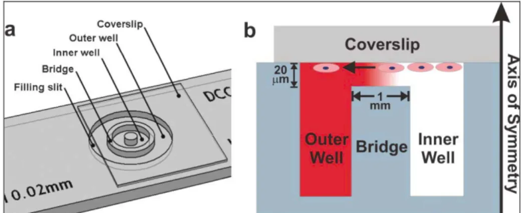
The Dunn Chamber device is very similar to the Zigmond Chamber, but is much less susceptible to evaporation [16]. In the Dunn chemotaxis Chamber (figure 1.3) the source and sink chambers are arranged as

concentric rings that can be filled with the appropriate solutions prior to affixing the glass coverslip seeded with cells.

Figure 1. 3 Dunn Chamber. (a) Structure of the device; (b) a gradient is formed in the 20 mm gap between the cell-seeded inverted coverslip and the glass bridge. Cell responses can be directly visualized in the bridge region [3].

When the coverslip is inverted and clamped, it seals both chambers and eliminates the air–liquid interfaces that contribute to evaporative losses. Although the gradient generated in the Dunn Chamber is less susceptible to evaporation, its advantages and disadvantages are similar from those of the Zigmond Chamber. The gradient is pseudo-steady state for periods of time up to 1–2 h, and it can be calculated for all time points and biomolecule concentrations. Like the previous chamber, the Dunn Chamber also has a ridge region that allows cell responses to be imaged directly and correlated with specific gradient characteristics. The gradients are short-lived and time-evolving, and cannot be modified once solutions are loaded and the coverslip is secured. Like the Boyden Chamber/Transwell Assay and the Zigmond Chamber, the Dunn Chamber is only capable of generating multi-factor combinatorial gradients along a single axis. The only major difference among these system is their geometric symmetries: from a practical point of view, evaluating the cell response from a radially symmetric design is slightly more difficult since cells must be tracked using polar instead of Cartesian coordinates. Tracking cells along a single axis, as in the Zigmond Chamber, is more straightforward.

In later times different solutions to produce a biomolecular gradient were proposed. In some applications related to tissue engineering, as found in Boland et al. works [17], the simplest method to produce a biomolecule gradient is the use of a hydrogel matrix: generally it is made of biological substances such as collagen, fibrin or agarose where cells can be seeded. The biomolecule is deposited on the matrix surface and then it diffuses inside it, generating a concentration gradient over the cells. The gradient evolves in both space and time (figure 1.4).

Figure 1. 4 Error-function solution of the concentration profiles generated at 5 min intervals for a biomolecule diffusing away from a constant concentration source using an assumed diffusivity of D = 6.4 x 10-7 _cm2_s-1 _[3].

This method is very popular because hydrogels are easy to make and provide cells with an environment that is quite similar to in vivo tissue. Moreover, the high network density of the gels allows the movement of chemical species to occur only via free diffusion, unaffected by the bulk fluid movement around the gel. Unfortunately the biological hydrogel method offers reduced control over the spatiotemporal evolution of the gradient and generates gradients with poor reproducibility. Moreover, lack of spatial and temporal gradient control is caused by the fact that the diffusion of chemical species in hydrogel is determined strictly by the chemistry of the polymer chains and the network porosity of the gel. An additional series of problems is related to the optical properties of some gels that make it difficult to distinguish the cell from the hydrogel

background. An example is given by collagen gels, which have ordered fibrils that refract incident light and interfere with phase contrast microscopy.

Some of the mentioned problems are overcome by the use of glass micropipettes, most commonly associated with the work of Mu-Ming Poo’s group [18]. In this method, a capillary glass is heated and pulled axially, forming a fine glass tip with an internal diameter of approximately 1 μm. This micropipette is filled with a biomolecule solution which can be pneumatically ejected out into the extracellular environment (figure 1.5).

Figure 1. 5 Typical micropipettes for electrophysiology loaded with soluble molecules mounted in micromanipulators, arranged around the cell culture dish [3].

The frequency of the puffs and the volume ejected with each puff are determined by the pneumatic pump frequency and driving pressure. The puffs combine to form a diffusive gradient that diffuses in radial direction from the micropipette tip. The second difference of the micropipette method is that, instead of being pneumatically ejected, the biomolecule solution is simply allowed to passively diffuse from the micropipette tip [19]. The micropipette method readily generates gradients and elicits responses from a variety of cell types including neutrophils [19] and primary neurons [18].

Figure 1. 6 Attractive turning response of an axon toward the gradient of netrin-1. The gradient was produced by the pulsatile application of a solution, containing netrin-1, from a micropipette [10].

Unlike biological hydrogels, the micropipette method is well suited for characterizing single cell responses since cells are cultured in standard cell culture dishes and can be observed with traditional optical microscope. The gradient can be oriented at a specific angle and distance relative to the cell to provide a more quantitative assessment of the response of the cell to the gradient. Multiple micropipettes can be placed around cells [20] and, in principle, could be used to generate multifactor combinatorial gradients. Like the biological hydrogel method, micropipettes can not generate highly reproducible or controllable gradients. As the biomolecule gradient is formed in free solution small vibrations, thermal imbalances, or evaporation can cause convective currents, distorting the gradient during the course of an experiment.

1.3.2 The microfluidic methods

The microfluidic researches are focused on the need of better gradient-generating methods in order to have a quantitative gradient characterization and an experimental reproducibility. Generally, microfluidic methods use microfabrication tools to fabricate cell culture environments with micrometer precision.

One of the easiest ways to create quantified gradients is the selective absorption of biomolecule on the cell culture substrate, and different

Delamarche and colleagues [21], and modified by Fosser and Nuzzo [22], employs a microfluidic channel with a reservoir at one or both ends. A biomolecule solution is dispensed into the reservoir at one end of an empty or liquid-filled channel. The solution is drawn into an empty channel via capillarity [21], or diffuses into a pre-filled channel [22] and adsorbs non-specifically to the internal surfaces. Philipsborn and colleagues [23] used micro contact printing to deposit proteins. By controlling the spacing and density of high-resolution protein patterns, they were able to closely approximate continuous gradients with different slopes and concentration ranges. These patterns were used to study the response of chick temporal retinal axons to gradients of ephrin-A5 [24]. In each of these methods the gradient stability is always affected by the biomolecule’s binding to the substrate and the chemical reactions that occur between patterned biomolecules and chemical components of the cell culture medium. Among the advantages of producing a gradient with the adsorbed molecules, there are: the possibility to have quite stable gradient, no complex labor-intensive fabrication step, a greater control over the gradient geometry. Some drawbacks of these methods rely on the denaturation of adsorbed biomolecules due to the interaction with cell culture medium during the whole experiment.

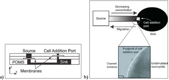
Other microfabrication methods allow the creation of gradient generators which can actively control the chemical species within the device: the time evolving and the steady state gradient generators. In the former type of generators, the gradient has a limited lifetime and it is determined solely by the diffusion coefficient of biomolecule and by the geometry of the device. Abhyankar and colleagues [25], for example, developed a device that generates quantifiable gradients capable of eliciting chemotactic responses from cells. It consists of three layers in a lollipop configuration (figure 1.7 a). The inlet for the biomolecule source solution near the stem of the lollipop is separated from the gradient chamber in the bottom layer by a

polyester membrane perforated with 200 nm-diameter holes (figure 1.7 b). The cell addition inlet, located near the elliptical gradient sink, is separated from the gradient-forming region by a similar membrane, but one containing 10 mm diameter holes.

a) b)

Figure 1. 7 a) A cross-section schematic of the device shows the polyester track

etch membranes encapsulated in three layers of PDMS; b) Cells loaded into the

cell addition port attached to the floor of the sink region and migrated towards the source region in response to a gradient of the bacterial peptide f-met-leu-phe (fMLF) (adapted from [25]).

Since the source and sink concentration are not actively maintained, the device is limited to time-evolving gradients and can not control the gradient’s spatiotemporal evolution once the gradient fluids have been loaded. Although it was not demonstrated by Abhyankar and colleagues, the design of the system could be extrapolated to generate multiple independent gradients with various orientations and positions. However, this system is not suitable for all gradient studies, especially those requiring long-term gradient exposure.

The time evolving gradient generators [25], [26] are easy to characterize mathematically and quantitatively but they are suited only in short term gradient studies of cells, excluding experiments such as: cell/progenitor cell differentiation, cell growth and proliferation. On the contrary the steady state gradient generators create and maintain a wide

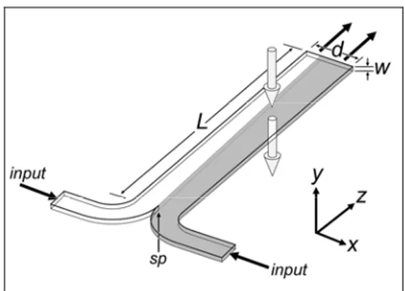
variety of steady state gradients for periods of time limited only by the supply of reagents. These systems can create complex geometries of gradients, but high reagent consumption and high shear stresses are avoiding their widespread use. The simplest system of this group is the so-called T-sensor [27] (figure 1.8).

Figure 1. 8 Conceptual rendering of the operation of the T-sensor. Two fluids enter through input channels, merging at the stagnation point (sp). As depicted in this figure, the fluid on the right contains a diffusible analyte (gray) that spreads across the d-dimension as flow proceeds along the channel length. Typical measurements are made by fluorescence detection along the optical axis, denoted with large arrows in the y-direction.

The system generates steady-state gradients that are reproducible and can be characterized quantitatively. Cells growth within the device can be visualized using standard microscopy and their development, differentiation, or migration can be correlated with specific gradient characteristics due to the temporal stability of the gradient. Constant perfusion prevents depletion of nutrients and accumulation of cell waste, allowing cells to be maintained for long periods of time in culture. The position and shape of the gradient can be modulated dynamically by adjusting the inlet flow rates and solution concentrations, respectively. Disadvantages of continuous fluid flow include high reagent consumption, exposure of cells to confounding and potentially damaging mechanical forces, all characterized by T-sensor devices. In addition, T-sensor devices

can only generate single-solute, sigmoid-shaped gradients or multi-factor gradients in which each biomolecule solution acts as the sink for the other. The gradients are also confined to a single axis perpendicular to the direction of fluid flow, precluding more complex gradient environments. This limit is overcome by the device developed by Jeon and colleagues [28] which is based to the T-sensor concept but forms more complex gradients. The complexity is achieved by the recombination of the inlet fluids in an upstream microfluidic mixer (figure 1.9).

Figure 1. 9 2D schematic of the device with 3D exploded view of the gradient generated downstream of the microfluidic mixer [3].

Flow rates of steady state gradient generators are about 1 μl min-1and this

can represent a drawback for those experiments that do not require any mechanical forces imparted on cells. In order to overcome problems of shear stress caused by fluid, some gradients generators use different solutions to the detriment of complex form of gradient, as in example proposed by Wu and colleagues [29] where a hydrogel matrix divides the fluid reservoir from the cells seeding area. Moreover, current generators are mono directional and can not generate more complex chemical environments containing gradients with various positions and orientations. The great advantage of these systems relays on the fact that they can be integrated with patterned substrate to give cells topological stimuli, in order to make the experiments more similar to the in vivo conditions, or to

Tourovskaia and colleagues [30] designed a microfluidic device integrated with a micropatterned surface and used it to mimic spatial cues in myoblasts differentiation process for muscle cell assembly. It allowed to confine the fusion of myoblasts into aligned, isolated multinucleated myotubes. Wang and colleague realised a microfluidic system where the substrate is modified in order to obtain surface-bound guidance cues that mimic the conditions of the growth cones realistically [31]. Ree and colleagues [32] used the patterning of surface to expose cells to a specific well-controlled fluidic microenvironment. Makiko Goto and colleagues [33] integrated a microchip with micro and nanometer scale patterned surface to investigate and observe the behaviour of fibroblasts.

1.4 THE MICROFLUIDIC MULTI-INJECTOR (MMI)

The microfluidic system, developed by Chung and colleagues [34] belongs to the time evolving gradient generators group. It is a system that replicates the micropipette method [10], [18] in a microfluidic platform but which is able to produce stable gradients.

In the MMI gradient generator (figure 1.10) a biomolecule solution is pneumatically ejected out of a microchannel orifice that is 10 μm wide. Pneumatic fluid ejection is controlled by a pneumatically-operated on-chip diaphragm valve, fabricated in PDMS using the Multilayer Softlithography.

Figure 1. 10 Schematic design of the Microfluidic Multi-Injector (MMI). Control channel and fluidic channel crossings make up the on-chip barrier valves (V1, V2, V3). These valves were actuated by pressurizing the control channel and deforming the membrane between the channels to close the fluidic channel.

These valves controlled the pulsatile release of solution into the reservoir to

generate a gradient. The micrograph shows the region around the barrier valve and the microfluidic orifice [33].

Stacked pulses of biomolecule solution diffuse away from the orifice, forming a gradient in the cell culture chamber. This gradient reaches the steady state, being the volume delivered at every ejection very low respect to the volume of the whole reservoir. Valve opening times and frequency can be optimized to avoid any rippling fluctuations in gradients. Figure 1.11 shows the development of a stable gradient as a function of time for valve actuation at 0.67 Hz with 1 s opening.

Figure 1. 11 The 2D fluorescence intensity profiles at various times after the start of pulsatile release [33].

The gradients are formed within 10 min and lasted as long as 2–3 h, making the MMI best suited for fast responding cell types. The measured fluorescence intensity profiles after 10 and 30 min fit well with the diffusion profile predicted by simulation (figure 1.12).

Figure 1. 12 1D normalized fluorescence intensity profile along a horizontal line of figure 1.11 [33].

The primary advantage the MMI device offers over the traditional methods, like the micropipette, is better reproducibility and quantification due to the precise dimensions of the device. Moreover, like the other microfluidic devices discussed so far, the MMI is also optically transparent, allowing observation of single cell responses, indirect gradient quantification using fluorimetric dyes, and the opportunity to establish correlations between the two. This device is also capable of producing two identical gradients, or two different competing gradients, simultaneously through a multiple injector geometry. However, like the micropipette method, the MMI gradient generator offers little control of the gradient during operation.

Compared to the steady-state gradient generators, the system does not generate such complex gradient form. In addition, the precise dimensions and the fixed position of the orifice relative to the cell culture chamber may improve the reproducibility of the generated gradient, but it comes at the expense of lost flexibility in positioning the source relative to the cell.

REFERENCES

[1] W. J. Rosoff, J. S. Urbach, M. A. Esrick, R. G. McAllister, L. J. Richards and G. J. Goodhill, A new chemotaxis assay shows the extreme sensitivity of axons to molecular gradients, Nat. Neurosci., 7: 678–682, 2004.

[2] R. W. Gundersen and J. N. Barrett, Neuronal chemotaxis: chick dorsal-root axons turn toward high concentrations of nerve growth factor, Science, 206(4422): 1079–1080, 1979.

[3] Thomas M. Keenan and Albert Folch, Biomolecular gradients in cell culture systems Folch, Lab Chip, 8: 34 – 57, 2008.

[4] A. Folch and M. Toner, Microengineering of cellular interactions, Annu.

Rev. Biomed. Eng., 2: 227–256, 2000.

[5] G. M. Whitesides, The origins and the future of microfluidics, Nature 442: 368-373, 2006.

[6] P. Castrataro, Microfluidic systems: AC electro-hydrodynamics of binary electrolytes and DNA microfluidic synthesizer, Doctoral Thesis, 2007. [7] T. M. Squires and S. R. Quake, Microfluidics: fluid physics at the nanoliter scale, Reviews of modern physics, 77: 977-1026, 2005.

[8] J. C. McDonald and G. M. Whitesides, Poly(dimethylsiloxane) as a material for fabricating microfluidic devices, Accounts Chem. Res., 35: 491– 499, 2002.

[9] T. M. Pearce, J. C. Williams, Microtechnology: Meet neurobiology, Lab

Chip, 7: 30-40, 2007.

[10]J.l El-Ali, P. K. Sorger and K. F. Jensen, Cell on chip, Nature, 442: 403-411, 2006.

[11] L. D. Landau and E. M. Lifshitz, Fluid Mechanics, Vol. 6, Pergamon Press, 1959.

[12] R. B. Bird, W. E. Stewart and E. N. Lightfoot, Transport phenomena, Wiley, New York, 1960, p. 780.

[13] T. M. Keenan, C. H. Hsu and A. Folch, Microfluidic ‘‘jets’’ for generating steady-state gradients of soluble molecules on open surfaces,

Appl. Phys. Lett, 89(11), 2006

[14] S. Boyden, The chemotactic effect of mixtures of antibody and antigen on polymorphonuclear leucocytes, J. Exp. Med, 115: 453–466,1962.

[15] S. H. Zigmond, Ability of polymorphonuclear leukocytes to orient in gradients of chemotactic factors, J. Cell Biol., 75(2 Pt 1): 606–616, 1997. [16] D. Zicha, G. Dunn and G. Jones, Analyzing chemotaxis using the Dunn direct-viewing chamber, Methods Mol. Biol., 75: 449–45, 1997.

[17] T. Boland, T. Xu, B. Damon and X. Cui, Application of inkjet printing to tissue engineering, Biotechnol. J., 1(9): 910–917, 2006.

[18] G. L. Ming, S. T. Wong, J. Henley, X. B. Yuan, H. J. Song, N. C. Spitzer and M. M. Poo, Adaptation in the chemotactic guidance of nerve growth cones, Nature, 417(6887): 411–418, 2002.

[19] G. Servant, O. D. Weiner, P. Herzmark, T. Balla, J. W. Sedat, H. R. Bourne, Polarization of chemoattractant receptor signaling during neutrophil chemotaxis, Science, 287(5455): 1037–1040, 2000.

[20] R. M. Fitzsimonds, H. J. Song and M. M. Poo, Propagation of activity-dependent synaptic depression in simple neural networks, Nature, 388(6641): 439–448, 1997.

[21] E. Delamarche, A. Bernard, H. Schmid, A. Bietsch, B. Michel and H. Biebuyck, Microfluidic networks for chemical patterning of substrate: Design and application to bioassays, J. Am. Chem. Soc., 120(3): 500–508, 1998.

[22] K. A. Fosser and R. G. Nuzzo, Fabrication of patterned multicomponent protein gradients and gradient arrays using microfluidic depletion, Anal. Chem, , 75(21): 5775–5782, 2003.

[23] A. C. von Philipsborn, S. Lang, A. Bernard, J. Loeschinger, C. David and D. Leh, Microcontact printing of axon guidance molecules for generation of graded patterns, Nat. Protoc., 1(3) 1322–1328, 2006.

[24] A. C. von Philipsborn, S. Lang, J. Loeschinger, A. Bernard, C. David, D. Lehnert, F. Bonhoeffer and M. Bastmeyer, Growth cone navigation in substrate-bound ephrin gradients, Development, 133(13): 2487–2495, 2006. [25] V. V. Abhyankar, M. A. Lokuta, A. Huttenlocher and D. J. Beebe, Characterization of a membrane-based gradient generator for use in cell-signaling studies, Lab Chip, 6(3): 389–393, 2006.

[26] C. W. Frevert, G. Boggy, T. M. Keenan and A. Folch, Measurement of cell migration in response to an evolving radial chemokine gradient triggered by a microvalve, Lab Chip, 6(7): 849–856, 2006.

[27] A. E. Kamholz, B. H. Weigl, B. A. Finlayson and P. Yager, Quantitative analysis of molecular interaction in a microfluidic channel: the T-sensor, Anal. Chem., 71(23): 5340–5347, 1999.

[28] N. L. Jeon, S. K. W. Dertinger, D. T. Chiu, I. S. Choi, A. D. Stroock, and G. M. Whitesides, Generation of solution and surface gradients using microfluidic systems, Langmuir, 16(22): 8311–8316, 2000.

[29] H. Wu, B. Huang and R. N. Zare, Generation of complex, static solution gradients in microfluidic channels, J. Am. Chem. Soc., 128(13) 4194– 4195, 2006.

[30] A. Tourovskaia, X. Figueroa-Masot and A. Folch, Differentiation-on-a-chip: A microluidic platform for long-term cell studies, Lab Chip, 5: 14-19, 2005.

[31] C. J.Wang, X. Li, B. Lin, S. Shim, G-L Ming and A. Levchenko, A microfluidic-based turning assay reveals complex growth cone responses to integrated gradients of substrate-bound ECM molecules and diffusible guidance cues, Lab Chip, 8: 227-237, 2008.

[32] S. W. Rheea, A. M. Taylora, C. H. Tub, D. H. Cribbsb, C. W. Cotmanb and N. L. Jeon, Patterned cell culture inside microfluidic devices, Lab Chip, 4: 2004.

[33] M. Goto, T. Tsukahara, K. Sato and T. Kitamori, Micro- and nanometer-scale patterned surface in a microchannel for cell culture in microfluidic devices, Anal Bioanal Chem 390: 817-823, 2008.

[34] B. G. Chung, F. Lin and N. L. Jeon, A microfluidic multi-injector for gradient generation, Lab Chip, 6(6): 764–768, 2006.