UNIVERSITY of PISA
PhD COURSE in
Molecular, metabolic and functional exploration of the nervous system and the sense organs
(SSD BIO/12)
A COMPARISON OF META-ANALYSIS METHODS FOR DETECTING
DIFFERENTIALLY EXPRESSED GENES IN MICROARRAY EXPERIMENTS:
AN APPLICATION TO MALIGNANT PLEURAL MESOTHELIOMA DATA
Candidate
Supervisor
Dr. Manuela Di Russo
Dr. Silvia Pellegrini
ABSTRACT
The proliferation of microarray experiments and the increasing availability of relevant amount of data in public repositories have created a need for meta-analysis methods to efficiently integrate and validate microarray results from independent but related studies.
Despite its increasing popularity, meta-analysis of microarray data is not without problems. In fact, although it shares many features with traditional meta-analysis, most classical meta-analysis methods cannot be directly applied to microarray experiments because of their unique issues.
Several meta-analysis techniques have been proposed in the context of microarrays. However, only recently a comprehensive framework to carry out microarray data meta-analysis has been proposed. Moreover very few software packages for microarray meta-analysis implementation exist and most of them either have unclear manuals or are not easy to apply.
We applied four meta-analysis methods, the Stouffer’s method, the moderated effect size combination approach, the t-based hierarchical
studies on malignant pleural mesothelioma. We focused on differential expression analysis between normal and malignant mesothelioma pleural tissues. Both unfiltered and filtered data were analyzed. The lists of differentially expressed genes provided by each method for either kind of data were compared, also by pathway analysis. These comparisons highlighted a poor overlap between the lists of differentially expressed genes and the related pathways obtained using the unfiltered data. Conversely, a higher concordance of the results, both at the gene and the pathway level, was observed when filtered data were considered. The fact that a significant number of genes were identified by only one of the tested methods shows that the gene ranking is based on different perspectives. In fact, the analyzed methods are based on different assumptions and focus on diverse aspects in selecting significant genes. Since so far there is no consensus on what is (are) the ‘best’ meta-analysis method(s), it may be useful to select candidate genes for further analysis using a combination of different meta-analysis methods. In particular, differentially expressed genes detected by more than one method may be considered as the most reliable ones while genes identified by only a single method may be further explored to expand the knowledge of the biological phenomenon of interest.
1 INTRODUCTION
Microarray technology simultaneously measures the mRNA of tens of thousands of genes in biological samples in a high-throughput and cost-effective manner. Since its introduction in 1995 [1], microarray technology has improved dramatically and became a widely used tool to study the whole transcriptome of many organisms. It has been adopted to explore the molecular basis of fundamental biological processes and complex diseases [2, 3], to improve the disease taxonomy [4, 5], to classify patients into known disease subclasses [6], to analyze the response to drug administration [7], and to predict disease outcomes [8, 9].
Enhancements in microarray technology and its widespread use have led to the generation of a relevant amount of data and resulted in several large public data repositories such as Gene Expression Omnibus (GEO) [10] (http://www.ncbi.nlm.nih.gov/geo/) from NCBI, ArrayExpress [11] (http://www.ebi.ac.uk/arrayexpress/) from EBI and CIBEX (Center for Information Biology gene EXpression database) [12] (http://cibex.nig.ac.jp/).
same or similar biological questions. Hence there has been a growing interest in developing methods to efficiently integrate microarray data from independent studies with the aim of fully exploiting the rich information produced. Meta-analysis appears to be an effective solution to this pressing issue [13].
As stated by Hedges, “meta-analysis consists of statistical methods for combining results from independent but related studies” [14]. However the term meta-analysis is also widely used in a broader sense, as we do here, to indicate the whole process of identification, selection, assessment and quantitative synthesis of several studies concerning a well-defined research question [15]. Many people use the term meta-analysis interchangeably with systematic review, however not all the systematic reviews are meta-analyses. In fact a meta-analysis is a systematic review which provides a statistical synthesis of the results and produces an overall estimate of the effect of interest.
Meta-analysis offers several practical advantages.
First of all, meta-analysis represents an inexpensive solution to overcome the problem of reduced statistical power of microarray experiments and to reveal true effects of interest [16]. Typically, in microarray experiments many probes are investigated in few samples due to the high cost of this technology or the lack of biological replicates available. The straight consequence is that studies with small sample sizes are less likely to detect true effects and more prone to false positive and false negative results. Putting results together, therefore, increases the sample size and the statistical power of the study. It also allows a more accurate estimation of the effect, even if derived from small but consistent variations.
Moreover, meta-analysis has the potential to strengthen and extend the results obtained by individual studies and to increase their reliability. Indeed, it has been shown that microarray studies are poorly reproducible across platforms and/or laboratories [17, 18]. Technological differences among different microarray platforms [19], large variations in biological and experimental settings, small sample sizes and inappropriate statistical methods [20, 21] have been pointed out as the major sources that contribute to the inconsistency of microarray results. Many of these can be assessed and controlled or overcome by the use of standard reporting methods and the careful application of large-scale meta-analysis techniques with an appropriate statistical modeling of the inter-study variation [16].
Meta-analysis has been widely used in the area of medical and epidemiological research as well as in the sociological and behavioral sciences [22]. The applicability of meta-analysis methods to microarray datasets was demonstrated for the first time in 2002 by Rhodes who combined four datasets on prostate cancer to determine genes that were differentially expressed between clinically localized prostate tumor and benign prostate tissue samples [23]. Since then, several applications of meta-analysis to microarray data appeared in the literature [24-26].
Through a systematic search on PubMed, Tseng and colleagues [27] found that 333 microarray meta-analysis papers (including reviews, biological applications, methodological articles and database/software description papers) were published until December 2010, thus confirming the relevant interest of the scientific community in this challenging task. In more than half of the above mentioned publications, meta-analysis was
combined for classification analysis [31], to identify co-expressed genes or to build gene networks [32-34], to evaluate reproducibility and bias across studies [35-37]. Figure 1.1 illustrates a microarray meta-analyses summary performed by Tseng and colleagues [27].
Figure 1.1: Classification of the 333 microarray meta-analysis papers reviewed by
Tseng based on the type of paper (A) and the purpose of meta-analysis (B) (image modified from [27])
Despite its increasing popularity, however, meta-analysis of microarray data is not without problems. In fact, although it shares many features with traditional meta-analysis, most classical meta-analysis methods cannot be directly applied to microarray experiments because of their unique issues such as the large number of variables involved and the technical complexities of combining data across different experimental platforms (e.g. gene nomenclatures, species and analytical methods) [38].
1.1 AIM OF THE STUDY
In this study, we focused on the application of meta-analysis to the two-class comparison microarray experiments. The objective of this kind of studies is to identify DEGs between two well-defined conditions, namely cases and controls. Four statistical approaches were comparatively evaluated: the weighted version of the inverse normal method by Marot
proposed by Marot [40], both implemented in the R ( http://www.r-project.org/) package metaMA, the t-based hierarchical modeling described in Choi et al. [16] and implemented in the Bioconductor (http://www.bioconductor.org/) package GeneMeta [41] and the rank product method with the RankProd Bioconductor package [42]. These methods were applied to a set of three publicly available microarray studies on malignant pleural mesothelioma to identify DEGs between normal and malignant mesothelioma pleural tissues. Since it is not yet clear if filtering is beneficial from a meta-analysis perspective, both unfiltered and filtered data were analyzed to evaluate the impact of a common filtering strategy on meta-analysis results.
2 BACKGROUND
A considerable literature has been published to guide the whole review process and the meta-analysis for medical and epidemiological studies [43-45]. Moreover, some guidelines for the reporting of systematic reviews and meta-analyses, outlined in the Quality of Reporting of Meta-Analyses statement for randomized trials by QUORUM group [46] and its evolution into PRISMA (Preferred Reporting Items for Systematic Reviews and Meta-Analyses) [47], are universally accepted.
On the contrary, there is little guidance to carry out a meta-analysis of microarray datasets. The first attempt in this direction was represented by the paper of Ramasamy and colleagues who proposed a seven-step practical approach to conduct a meta-analysis of microarray datasets: “(1) Identify suitable microarray studies; (2) Extract the data from studies; (3) Prepare the individual datasets; (4) Annotate the individual datasets; (5) Resolve the many-to-many relationship between probes and genes; (6) Combine the study-specific estimates; (7) Analyze, present, and interpret results” [48]. Steps from 2 to 5 apply separately to the individual datasets.
Each step, in turn, consists of several critical points that will be highlighted and examined in detail in the following paragraphs.
2.1 IDENTIFICATION OF SUITABLE MICROARRAY STUDIES
A meta-analysis begins with a well-formulated objective. As highlighted in the introduction, meta-analysis of microarray studies can be used for several purposes, for example to identify DEGs between two or more groups, to identify co-expressed genes, to build gene networks or to evaluate reproducibility and bias across studies. In the following we will focus on meta-analysis for DEGs detection, however most of the considerations apply regardless of the specific topic.
The study selection process is guided by the definition of the inclusion/exclusion criteria. These criteria should be a priori established and should derive immediately from the objective(s) of the study. They can be based on biological (e.g. specific disease, type of outcome, type of tissues, organism) or technical issues (e.g., density of array, minimum number of arrays). A clear, detailed and unambiguous formulation of inclusion/exclusion criteria, possibly in the form of a real protocol, is essential to avoid the most frequent criticism of the meta-analysis, that is “mixing apples and oranges” [49].
Locating the studies is by far the most difficult and the most frustrating aspect of any meta-analysis but it is the most important and critical step. Many meta-analyses begin with a systematic literature search. Keywords concerning the research question and their synonyms are typically used to identify studies for inclusion in the review. In order to retrieve all the relevant studies on a given topic, the search should be as
main electronic databases of abstracts listed in Table 2.1. Reading the latest review articles and contacting specific investigators that are known to be active in the area can help to identify additional studies missed by automated search and ongoing research efforts with unpublished data.
Database Web site
Online repositories of abstracts
PubMed http://www.pubmed.gov/
Google Scholar http://scholar.google.com/
Web of Science (requires subscription) http://wos.mimas.ac.uk/
SCOPUS (requires subscription) http://www.scopus.com/
Microarray repositories recommended by MIAME for mandatory data deposition
Array Express http://www.ebi.ac.uk/arrayexpress/
CIBEX http://cibex.nig.ac.jp/
Gene Expression Omnibus (GEO) http://www.ncbi.nlm.nih.gov/geo/ Other useful sites for data identification
ONCOMINE http://www.oncomine.org/
Stanford Microarray Database (SMD) http://smd.stanford.edu/
Table 2.1: Useful web resources to identify suitable studies for microarray
meta-analysis (modified from [48])
Concerning microarrays, it is appropriate to extend the search to public microarray data repositories, as well as to a few more specialized databases, listed in Table 2.1. A quick review of the abstracts and experiments description is essential to eliminate those studies that are clearly not relevant to the meta-analysis or do not meet the specified selection criteria.
After the identification of candidate studies from abstracts, the articles or inherent information from authors, where available, have to be retrieved to confirm their eligibility. To limit the risk of compromising the quality of meta-analysis results, the included studies should undergo a quality assessment, that is an accurate evaluation of the study characteristics in terms of the study design, implementation and analysis [49]. In fact, if a meta-analysis includes many low-quality studies, then the
errors in the primary studies will be carried over to the meta-analysis, where they may be harder to identify, and the obtained result will be biased (“garbage in, garbage out“). Regarding microarray studies, the quality assessment should be performed at the study-level as well as at the data-level, as will be extensively described in the following paragraphs.
2.2 EXTRACTION OF THE DATA FROM STUDIES
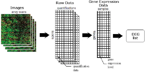
As illustrated in Figure 2.1, there are four levels of data arising from microarray analysis: (1) the scanned images, (2) the raw data or FLEO (Feature-Level Extraction Output) files [48], such as Affymetrix CEL and GenePix GPR files, that is the quantitative outputs from the image analysis software, (3) the Gene Expression Data Matrix (GEDM) arising from the application to raw data of preprocessing algorithms, which represents the gene expression summary for every probe and sample and (4) the list of genes that are declared as differentially expressed in the study.
According to the conclusions of the study of Suarez-Farinas [51] and the recommendations of Ramasamy [48], raw data represent the ideal input for meta-analysis because they are independent of the specific preprocessing algorithms used and can be converted to GEDMs in a consistent manner thus producing more comparable data. By contrast, using GEDMs as input for meta-analysis is unsuitable because they considerably depend on the choice of the preprocessing algorithms, which may produce non-combinable results. The same considerations apply to the lists of DEGs. In fact, even if DEGs lists are easier to obtain since they are often included in the main text or supplementary data of published microarray studies, they heavily depend on the preprocessing algorithms, the statistical methods and cutoffs, and the annotation system adopted in the original study.
In relation to the data retrieval phase there are three major problems: (1) the efficient access to microarray data, (2) their standardization, and (3) the comparability across platforms.
2.2.1 MICROARRAY STANDARDS AND REPOSITORIES
In the past years, most of the publicly available microarray data produced by different research groups worldwide were scattered in the web both as supplementary data of a published article and as links to the authors web pages. Consequently it was very difficult for the researchers to locate and systematically collect the relevant data available. This problem has been addressed and partially solved through the development of several public repositories. Today, many web databases exist. ArrayExpress from EBI and GEO from NCBI are the two largest ones: on 24 January 2013, GEO contained 35618 experiments and 870318
ArrayExpress. Several other microarray databases are housed in specific universities or groups, including Stanford Microarray Database (SMD) and RNA Abundance Database (RAD; http://www.cbil.upenn.edu/RAD [52]) from University of Pennsylvania, or are focused on particular organisms (e.g. yeast Microarray Global Viewer; http://www.trans criptome.ens.fr/ymgv/ [53]) or diseases (e.g. ONCOMINE and Cancer Genome Workbench (CGWB) [54]) [27, 55].
At the beginning the effectiveness and the use of these public databases were severely limited by two factors: (1) the incompleteness or the lack of experimental information needed to assess the quality of the data, to repeat a study or to reanalyze the data, and (2) the lack of standards for presenting and exchanging such data. A considerable improvement occurred with the publication of the Minimum Information About a Microarray Experiment (MIAME) [50] standard by the Microarray Gene Expression Data Society (MGED) (http://www.mged.org). MIAME guidelines describe the minimum information that has to be provided to enable the comprehension of the results of a microarray experiment and their validation by independent researchers. The information required by MIAME standard includes the experimental design, array design (e.g. platform type and provider, gene identifiers, probe oligonucleotides), details on samples and treatments applied (e.g. laboratory protocols for sample treatments, extraction and labeling), hybridization conditions, measurements and normalization controls (e.g., normalization techniques applied and control elements used to obtain the final processed data). The current MIAME standard requires the submission to public databases of both the FLEO and GEDM files [56].
journals have adopted MIAME guidelines as a requirement for the paper publication [57]. The availability of standardized microarray gene expression data in these public repositories: (1) greatly enhanced the accessibility, the retrieval and the sharing of the data; (2) increased the reliability of the data quality and (3) improved the comparability and integration of data from different laboratories in a meta-analysis perspective.
Despite the wide adoption of MIAME standard by public microarray repositories and scientific journals, only about one-third of published studies have their raw data deposited in public databases [58]. Moreover, even when data are available, the incomplete annotation and/or the lack of data processing and analysis description limit their usefulness for further analyses [59].
2.2.2 CROSS-PLATFORM COMPARABILITY
One major issue in meta-analysis of microarray datasets concerns the possibility of combining raw measurements from different microarray technologies.
Although all DNA microarrays are based on the hybridization of complementary nucleic acid strands, the available platforms differ in the manufacturing process, hybridization protocols, image and data analysis, making comparison of the data across platforms very difficult.
Based on the length of the probes, microarrays can be classified as: (a) cDNA arrays, using probes constructed with PCR products of up to a few thousands base pairs, (b) short oligonucleotide arrays, using short probes (25-30 mer), such as Affymetrix GeneChip
®
arrays (Santa Clara, CA, USA), and (c) long oligonucleotide arrays, such as those produced byvaries among microarrays. Long oligonucleotides are thought to mimic the properties of cDNA probes offering high sensitivity and good specificity, while giving better probe homogeneity. For both cDNA and long oligonucleotide arrays, typically one probe is designed for each gene that is to be probed [60]. In Affymetrix arrays, for each gene, a unique region is identified, then a set of 11–20 complementary probes spanning this region is synthesized. These complementary probes are referred to as ‘Perfect Match’ probes (PM). Each PM probe is then paired with a ‘Mismatch’ probe (MM), which has the same sequence as the PM except the central base replaced with a mismatched nucleotide. The complete set of PM and MM probe pairs for each gene is referred to as a ‘probe set’ [61].
Short oligonucleotides showed a higher specificity in target identification compared to long cDNA clones that were more prone to cross-hybridization [62].
Gene annotation can also contribute to platform differences. Gene expression values can be compared effectively across platforms only if genes are accurately identified on all platforms. Unfortunately, the lack of standardized annotation methods and of a regular update of annotations severely affect the cross-platform comparability. Moreover, the presence of poorly annotated and/or not specific probes on some arrays contribute to increase misalignments among platforms [63]. In any case, even if an accurate translation between different nomenclatures is achieved, the differences in how different platforms measure specific transcripts still remain and could have important impact on any attempt to conduct effective microarray data meta-analysis by increasing the false negative rate [38].
color or two-channel. In one-color microarrays, such as Affymetrix arrays, a single labeled RNA sample is hybridized on a chip thus providing an absolute measurement of expression in the given sample (absolute quantification). By contrast, expression levels measured by cDNA microarrays and long oligonucleotide platforms, using two-channel detection, are usually reported as a ratio of the signal from a target RNA sample relative to one from a co-hybridized sample (relative quantification) [1]. These different measurement strategies result in diverse experimental designs which complicate the direct comparison and integration of the data. The use of a common reference design for the two-channel platforms, where each experimental RNA sample is co-hybridized with a reference RNA sample, represents a valid solution as it closely reproduces the single-channel approach.
Finally, different preprocessing steps, such as quality filtering, background correction and normalization, adopted to transform the raw data into the corresponding gene expression values, have substantial influence on the data [64].
All these differences produce qualitatively different data whose comparability has been widely debated. See for references [19, 65-71].
2.3 PREPARATION OF THE INDIVIDUAL DATASETS
Once the raw data from individual studies have been collected, they have to be converted into GEDMs, which can then be used as input for the meta-analysis.
Before the preprocessing or transformation steps, Ramasamy [48] suggests to check the quality of the arrays in the individual studies to identify and remove those of poor quality. Microarray quality is assessed
by comparing suitable numerical summaries (e.g. average background, scale factors, percentage of present calls,) across microarrays, so that outliers and trends can be visualized and poor-quality arrays can be identified. There are many Bioconductor packages for quality assessment including arrayMagic [72] for the two-color technology platform, Simpleaffy [73] and affyPLM [74] for the Affymetrix platform and ArrayQualityMetrics [75] which manages many microarray technologies. Only the arrays that pass the quality check should be included in the meta-analysis.
At this point the data undergo different levels of transformation or preprocessing that are: background or mismatch subtraction, probe set summarization which combines multiple measures of the same transcript, normalization within and between arrays. As it is now widely known [76], using different raw data transformation methods leads to disagreements in the resulting DEGs even within one experiment on a single platform.
It is thus evident the need to consistently process the data to remove any systematic differences. The simplest case is when data from multiple studies the same platform have to be combined. In this case it is, in fact, sufficient to apply the same algorithm to all datasets. Much more often, however, researchers are faced with the problem of combining datasets from different platforms, which may have different designs and thus different preprocessing methods options. In this case, comparable preprocessing algorithms should be applied to the individual datasets. There are very few universally applicable preprocessing algorithms, such as the variance stabilizing normalization [77]. By contrast, it is more common to use different preprocessing methods for each platform.
different platforms [48]. However, it has been found that while the default procedures suggested by microarray manufacturers result in general slightly better accuracy, the results provided by alternative approaches, like those proposed by Bioconductor packages, are far more precise [70].
The identification and adjustment of any batch effects, especially in large microarray datasets, are also of great importance. Many different experimental features can cause biases including different sources of RNA, different microarrays print batches or platforms, as shown in Figure 2.2. Unsupervised visualization techniques such as Support Vector Machines (SVM) [78], Singular Value Decomposition (SVD) [79], Principal Component Analysis (PCA) [80] and the Distance Weighted Discrimination (DWD) method proposed by Benito and colleagues [81] can help to identify any grouping caused by experimental factors within microarray datasets.
Figure 2.2: A visualization of batch effect sources at each stage of a microarray
gene expression experiment (image from [82])
In single-study analysis it is common practice to filter out probes based on different criteria. Probes showing severe manufacturing or hybridization problems or a signal-to-noise ratio below a fixed threshold,
probes marked as ‘absent’ or showing little variation among experimental conditions are usually excluded or under-weighted from the successive analysis. To date, it has been demonstrated that filtering improves cross-platform reproducibility [21, 64, 67, 83] but it is not yet clear whether filtering is beneficial to meta-analysis.
Another problem that may occur in this phase deals with the management of possible within studies technical replicates. In fact, technical replicates cannot be considered as independent observations and should be aggregated taking, for example, the mean or median of the corresponding gene expression measurements.
Finally, one could check that the processed expression values from multiple platforms are comparable. Concerning this topic, one may use visualization techniques such as multidimensional scaling [84] to investigate for any clustering of arrays by studies.
2.4 ANNOTATION OF THE INDIVIDUAL DATASETS
The first step to combine different microarrays datasets is to find genes common to all arrays. The annotation of the individual datasets is a non trivial task because of the lack of a uniform nomenclature system and the many-to-many relationship between probes and genes.
Microarray manufacturers use specific probe-level identifiers (probe IDs) (e.g. Affymetrix probe ID) to identify the probes present on their own arrays. Moreover, different manufacturing techniques lead to the creation of multiple probes for the same gene. Therefore, one needs to identify which probes represent a given gene within and across platforms. In fact, even if the datasets share the same platform, the combination of different
conserved from version to version. In conclusion, to combine microarray datasets across studies a unique nomenclature must be adopted and all the different platform-specific IDs must be translated to a common identifier. There are many different options that could be used to this end. Genbank or RefSeq [63] accession number, Unigene ID [85] and Entrez ID [86] are the most common. Accession numbers are associated with specific transcripts, then there may be multiple per gene. Mapping between platforms on the basis of the accession number could produce an accurate result, as one can be confident that the probes are truly measuring the same entity; however, such an approach would be problematic as there would be many accession numbers for which probes only exist on one platform, greatly diminishing the ability to map between platforms. For this reason, mapping on the gene level is the most common choice. This allows to incorporate the information from many more probes, as it is much more likely to be able to find some probes associated with a gene for each platform than to find a probe associated with a specific accession number. Unigene and Entrez Gene have different strengths and weaknesses. While Unigene IDs may incorporate more information, it is very dynamic and is constantly being revised. Entrez IDs, on the other hand, are very stable and have been well-curated [87].
The problem of matching platform-specific probe IDs can be tackled in three ways. The traditional method is to use the annotation files provided by the manufacturers. The accuracy of these files was long criticized as the knowledge of the transcriptome is constantly growing. However, in recent years more and more manufacturers provide to release updated annotation files with varying degrees of regularity in an attempt to keep these annotations current.
Another option is to align the probe sequences provided by the vendors to a recent revision of either the Genome or the Transcriptome using the BLAST algorithm [88], trying to obtain more up-to-date gene-to-probe associations. It has been shown that cross-platform correlations improved using stringent sequence matching of the probes on the different platforms [89]. However, the probe sequences are not always available and this procedure can be computationally intensive and time-consuming for very large numbers of probes.
Alternatively, one can simply map probe IDs to a gene-level identifier (gene ID) such as Entrez ID or UniGene ID. Many published microarray meta-analyses [24, 26, 51, 90] have relied on UniGene ID to unify the different datasets, across platforms and array versions. The translation of the probe IDs to the corresponding gene IDs can be performed using either some Bioconductor annotation packages (e.g. annotate [Gentleman R. annotate: Annotation for microarrays. R package version 1.36.0.], annotationTools [91]) that aggregate the information from various platform-specific Bioconductor packages, or Web tools such as SOURCE [92] and RESOURCERER [93], MADGene [94], DAVID converter [95] and Onto-Translate [96]. The same mapping build, ideally the most recent, should be used for all datasets to avoid inconsistencies between releases [48].
Allen and colleagues [87] found that a BLAST alignment of the probes to the Transcriptome was more accurate than using the vendor’s annotation or Bioconductor packages. They also proposed a combination of all three methods (the “Consensus Annotation”) showing that it yielded the most consistent expression measurements across platforms.
some cases a probe could report to more than one gene and vice versa. Many probes can map to the same gene ID because of the clustering nature of the UniGene, RefSeq, and BLAST systems involved, or because the microarrays used contain duplicated probes. Vice versa, a probe may map to more than one gene ID if the probe sequence is not specific enough. Sometimes, a probe has insufficient information to be mapped to any gene ID. These probes should be removed from further analysis.
The simplest and even most stringent approach to solve these confounding situations is to use only the probes with one-to-one mapping for further analysis, thus excluding probes without a gene ID, probes mapping to multiple gene IDs and probes mapping to the same gene ID. Alternatively, probes with multiple gene IDs may be considered as independent gene expression measurements and be replaced by a new record for each gene, while multiple probes mapping to the same gene ID can be summarized using one of the following options: (1) selecting a probe at random, (2) taking the average of expression values across multiple probe IDs to represent the corresponding gene, (3) choosing the probe ID with the largest Inter Quartile Range (IQR) (or other similar statistics, such as standard deviation or coefficient of variation) of expression values among all multiple probe IDs to represent the gene. Although the option number 2 has been widely used due to its simplicity, IQR method is biologically more reasonable and robust and is highly recommended [97].
Recently, the MicroArray Quality Control (MAQC) project proposed another alternative. A single RefSeq ID was selected for each probe mapping to multiple RefSeq IDs, primarily the one annotated by TaqMan assays, or secondarily the one present in the majority of platforms. When
only the probe closest to the 3’ end of the RNA sequence was included [71].
The multiple gene expression datasets may not be very well aligned by genes and the number of genes in each study may be different. Therefore the common genes across multiple studies have to be identified and extracted. When a large number of studies were included in the meta-analysis, the number of genes common to all studies may be very small. At this point there are two possibilities: using only genes appearing in all datasets, or including also genes appearing in at least a pre-specified number of studies.
Having solved the many-to-many relationship by expanding and summarizing probes, one summary statistic per gene ID per study is available. The next step will be to combine the summary statistic for each gene ID across the studies using a meta-analysis technique.
3 STATISTICAL METHODS FOR
MICROARRAY DATA META-ANALYSIS
This chapter deals with the sixth step of Ramasamy’s guidelines for microarray meta-analysis. The choice of a meta-analysis method depends on the type of outcome (e.g. binary, continuous, survival), the objective of the study and the type of available data. As previously illustrated, we focused on the two-class comparison, the most commonly encountered application of meta-analysis to microarray data, whose aim is the detection of DEGs between two experimental groups or conditions.
There are two principal approaches to perform a meta-analysis, the relative and the absolute approach [98]. The relative meta-analysis is the most common one and is based on the calculation of a relative score expressing how each gene correlates to the experimental condition or phenotype of interest in each dataset. These scores are used to quantify the differences or similarities among studies and are integrated to find overall results (see Figure 3.1).
Figure 3.1: Stages of relative meta-analysis of microarray data (image from [13]) In contrast, in the absolute meta-analysis raw data from various microarray studies are integrated after transforming the expression values to numerically comparable measures. The derived data from the individual studies are normalized across studies and subsequently merged, thus enlarging the sample size and increasing the power of statistical tests. Traditional microarray data analysis is then carried out on the new merged dataset (see Figure 3.2) [13, 99].
Figure 3.2: Stages of absolute meta-analysis of microarray data (image from [13]) Although merging data can be attractive for its intuitiveness and convenience, cautions have to be taken since normalizations do not guarantee to remove all cross-study differences. There are few examples of studies where the absolute meta-analysis has been applied [31, 100, 101]. Contrary to relative meta-analysis, which is always possible for cross lab, platform and even species comparisons, absolute meta-analysis usually considers studies from the same or similar array platform [102, 103]. The collection of datasets from only one platform allows to pre-process and normalize data using the same method on all samples simultaneously.
In recent years several relative meta-analysis methods have been proposed using different approaches. There are four generic ways of combining information for DEGs detection:
1. Vote counting 2. Combine p-values 3. Combine effect sizes 4. Combine ranks.
They differ in the type of statistics measures proposed to summarize the study results.
3.1 VOTE COUNTING
Vote-counting is the simplest of the above approaches. For each gene, vote counting simply counts the number of studies in which a gene has been claimed significant [104]. To provide a statistical basis to vote counting techniques results, one can either calculate the significance of the overlaps using the normal approximation to binomial as described in Smid and colleagues [105] or calculate the null distribution of votes using random permutations [24]. For very small numbers of studies (usually 2– 4), the results can be summarized using a Venn diagram which displays the intersection and union distribution of DEGs lists detected by each individual study. In literature, it is well known that vote counting is statistically inefficient [14]. Moreover, vote counting does not yield an estimate of differential expression extent and the results highly depend on the statistical methods used in individual analyses. On the other hand, vote counting is useful when raw data and/or p-values for all genes are not accessible while only the lists of DEGs are available for each study.
Vote counting in the context of microarrays has been used successfully by Rhodes and colleagues [24], who applied it to identify a shared gene expression signature across cancer subtypes. First t-tests were calculated by comparing the treatment and control group in each study. Then, a binary score was assigned to each gene in each study based on whether its p-value passed a threshold (vote = 1) or not (vote = 0). Finally, a simulation of the likelihood of obtaining k or fewer votes (where k is the number of studies included) was done to estimate a significance level.
3.2 COMBINING P-VALUES
Combining p-values from multiple studies for information integration has long history in statistical science. Methods based on the combination of p-values are easy to use and provide more precise estimates of significance. However these methods do not indicate the direction (e.g. up or down regulation) nor the extent of differential expression. Moreover the results highly depend on the statistical methods used in individual analyses. Nevertheless, integration of p-values does not require that different studies use the same measurement scales therefore it is possible to combine results from studies realized by completely different technologies.
Several methods exist for combining p-values from independent tests; below, four p-value combination methods used in the context of microarray meta-analysis are briefly described.
3.2.1 FISHER’S METHOD
Fisher’s method [106] computes a combined statistics from the log-transformed p-values obtained from the analysis of the individual datasets:
(1) (∏ )
where pgi is the unadjusted p-value from one-sided hypothesis testing for gene g and study i and k being the number of individual combined studies. The meta-analysis null hypothesis is that all the separate null hypotheses, are true, whereas the alternative hypothesis is that at least one of the separate alternative hypotheses is true. Assuming independence among studies and p-values calculated from correct null distributions in each study, Sg follows a chi-square distribution with 2k degrees of freedom under the joint null hypothesis of no differential expression, thus p-values of the combined statistics can be calculated for each Sg. Alternatively, statistical inference can be done non-parametrically using a permutation approach. As there are many genes, p-values of the summary statistics must be corrected for multiple testing using one of the available procedures such as the Bonferroni correction, the false discovery rate (FDR) proposed by Benjamini and Hochberg [107] or its modified version proposed by Storey [108]. Finally, a threshold is chosen and two meta-lists, that are the lists of DEGs resulting from the meta-analysis, of over and under-expressed genes are reported. It is worth pointing out that Fisher’s product should be applied to p-values for up and down regulation separately. Using p-values from two-sided testing means ignoring the direction of the significance and may lead one to select genes that are
Rhodes and colleagues [23] were the first who applied Fisher’s method to microarray data. They identified a meta-signature of prostate cancer combining the results of four studies performed on different platforms.
Some variations to Fisher’s method have been proposed that give different weights to p-values from each dataset. Weight assignment can depend on the reliability of each p-value based on the data quality. Recently, Li and Tseng [110] introduced an adaptively weighted Fisher’s method (AW) where the weights are calculated according to whether or not a study contributes to the statistical significance of a gene. Li and Tseng showed the superior performance, in terms of power, of their AW statistics compared to Fisher’s equally weighted and other p-values combination methods, like Tippett’s minimum p-value [111] and Pearson’s (PR) statistics.
3.2.2 STOUFFER’S METHOD
Instead of log-transformation, Stouffer’s method [112] uses the inverse normal transformation. Unlike the Fisher’s method, which requires to treat over and under-expressed genes separately, the inverse normal method is symmetric in the sense that p-values near zero are accumulated in the same way as p-values near one [14]. In the Stouffer’s method, the one-sided p-values for each gene g from k individual studies are transformed into z scores and then combined using the following expression:
(2) ∑ ⁄√
where φ-1( ) is the inverse cumulative distribution function of standard normal distribution. Under the null hypothesis, the z statistic follows a normal N(0,1) distribution and therefore a p-value for each Z
can be calculated from the theoretical normal distribution. Finally, to take into account multiple comparisons, the FDR or other multiple testing correction methods can be applied. An alternative to (2) is to use the weighted method proposed by Marot and Mayer [39] which is implemented in the R package metaMA. Here:
(3) ∑ ⁄√ and
(4) √ ⁄ ∑ being ni the sample size of study i.
3.2.3 MINP AND MAXP METHODS
In the minP [111] and maxP [113] methods, for each gene, the minimum or maximum p-values over different datasets are taken as the test statistics. Smaller minP or maxP statistics reflects stronger differential expression evidence, however while minP declares a gene as differentially expressed if it is in any of the studies, maxP tends to be more conservative considering as differentially expressed only genes that have small p-values in all studies combined.
Combining p-values are techniques that in theory could use the published lists of DEGs, but may not be able to do so in practice. For example, most publications report the significant genes based on two-sided values, while the aforementioned methods require one-two-sided p-values. So it is preferable to use the raw data to minimize the influence of different methods across datasets.
3.3 COMBINING EFFECT SIZES
Methods based on the combination of effect sizes have been the most common approach to the meta-analysis of microarray studies. In statistics, an effect size is a measure of the strength of a phenomenon [114] (e.g. the relationship between two variables in a statistical population) or a sample-based estimate of that quantity. In general, effect sizes can be measured in two ways:
1. as the standardized difference between two means, or 2. as the correlation between the two variables [115].
Standardized Mean Difference (SMD) is the difference between two means, divided by the variability of the measures. Effect sizes based on SMD include Cohen’s d [116], Hedges’ g [14], and Glass’s delta. All three employ the same numerator (i.e. the difference between group means) but different estimates of the variability at the denominator [117].
An effect size approach is effective for microarray data application. First it provides a standardized index. At present, the measure of expression levels is not interchangeable in particular between oligonucleotide arrays and cDNA arrays. cDNA microarrays report only the relative change compared to a reference, which is rarely standardized. Obtaining effect sizes facilitates the combining of signals from one-color and expression ratios from two-color technology platforms. Second, it is based on a well-established statistical framework for the combination of different results. Third, it is superior to other meta-analytic methods in that it has the ability to manage the variability between studies. Moreover, in comparison to the p-values summary approaches, combining effect sizes gives information about the magnitude and direction of the effect.
In meta-analysis, the basic principle is to calculate the effect sizes in individual studies, convert them to a common metric, and then combine them to obtain an average effect size. Once the mean effect size has been calculated it can be expressed in terms of standard normal deviates (Z score) by dividing the mean difference by its standard error. A significance p-value of obtaining the Z score of such magnitude by chance can them be computed.
Without loss of generality, we can assume that we are comparing two groups of samples, such as treatment (t) and control (c) groups, in each study i=1,2,..k. For each study i, let and denote the number of samples in treatment and control group, respectively, with . Let and represent the raw expression values for gene g in conditions t and c for study i and replicate r and and be the corresponding log-transformed values. The data are assumed to be normally distributed as and ( ) In a microarray experiment with two groups, the effect size refers to the magnitude of difference between the two groups’ means. There are many ways to measure effect size for gene g in any individual study [118]. The SMD proposed by Cohen is defined as:
(5) ( ̅ ) ⁄
where ̅ and are the sample means of logged expression values for gene g in treatment (t) and control (c) group, in the ith study, respectively and is the pooled standard deviation:
where and denote the sample variances of gene g's expression level in the treatment and control groups, respectively.
Alternatively the SMD proposed by Hedges and Olkin [14] may be used. Hedges and Olkin showed that the classical Hedges'g overestimates the effect size for studies with small sample sizes. They proposed a small correction factor to calculate an unbiased estimate of the effect size which is known as the Hedges’ adjusted g and is given by:
(7) ( )
The estimated variance of the unbiased effect size is given by: (8) ( ) ( )
Then the effect size index (or its unbiased version) across studies is modeled by a hierarchical model:
(9) {
where is the average measure of differential expression across datasets for each gene g, which is typically the parameter of interest, is the between-study variance, which represents the variability between studies, and is within-study variance, which represents the sampling error conditioned on the ith study. The model has two forms: a fixed effect model (FEM) and a random effect model (REM), and the choice depends on whether between-study variation is ignorable. A FEM assumes that there is one true effect common to all studies included in a meta-analysis and that all differences in observed effect sizes are due to
contrast, in REM each study further contains a random effect that can incorporate unknown cross-study heterogeneity in the model. Thus ∼
N( , ) and ∼ N( , ).
To determine whether FEM or REM is most appropriate, the Cochran’s Q statistic [119] may be used to test homogeneity of study effect, which is assessing the hypothesis that is zero. Q statistic is defined as:
(10) ∑ ̂
where is the statistical weight and
(11) ̂ ∑
∑
is the weighted least squares estimator of the average effect size under the FEM which ignore the between-study variance. Under the null hypothesis of homogeneity (i.e. = 0), Q follows a chi-square distribution with k-1 degree of freedom. A large observed value of the Q statistics relative to this distribution suggests the rejection of the hypothesis of homogeneity, which should indicate the appropriateness of the REM. It must be noted that this homogeneity test has low power [120] and non-significant results do not imply that true homogeneity exists. If the null hypothesis of = 0 is rejected, one method for estimating is the method of moments developed by DerSimonian and Laird [121]:
(12)
̂
{
(13)
̂
∑ ∑ and (14)
(
̂
)
∑where ̂ is the statistical weight under REM.
The z statistic to test for DEGs under REM is then constructed as follows:
(15) ̂ √ (⁄ ̂ )
The z statistic for FEM is the same as that for REM except that = 0. To evaluate the statistical significance of the combined results, the p-values can be obtained from a standard normal distribution N(0,1) using these Z scores. For a two-tailed test, the p-value for each gene is given by:
(16) ( )
where is the standard normal cumulative distribution. To assess the statistical significance not assuming normal distribution, empirical distributions may be generated by random permutations. In both cases, the p-values obtained are unadjusted values which should be corrected to take into account the multiple comparisons.
Choi and colleagues [16] were among the first who applied these models to microarray meta-analysis. To estimate the effect size they considered the unbiased estimator of the SMD defined in equation (7) where was obtained from the standard t statistics for each gene from each individual dataset via the relationship:
(17) ⁄√ ̃
with ̃ ⁄ .
To estimate the statistical significance simultaneously addressing the multiple testing problem, Choi and colleagues adapted the core algorithm of Significance Analysis of Microarrays by Tusher and colleagues [122]. Column-wise permutations were performed within each dataset to create randomized data and z scores under the null distribution, for permutation b = 1, 2, …B. The ordered statistics ( ) and ( ) were obtained and the FDR was estimated for a
given gene by:
(18)
⁄ ∑ ∑ (
)
∑ ( )
where I(·) is the indicator function equal to 1 if the condition in parentheses is true, and 0 otherwise. The denominator represents the number of genes called significant in real data. The numerator is the expected number of falsely significant genes and given by the mean number across B permuted data. Integration of data using this meta-analysis method facilitated the discovery of small but consistent expression changes and increased the sensitivity and reliability of analysis. Later, Hong and Breitling [109] found that this t-based meta-analysis method greatly improved over the individual analysis, however it suffered from potentially large amount of false positives when p-values served as threshold.
version 1.30.1] where both alternatives to evaluate the statistical significance of the combined results are available.
Different variations of effect size models have also been developed by other research groups. Hu and colleagues [123] presented a measure to quantify data quality for each gene in each study where the quality index measured the performance of each probe set in detecting its intended target. As they used Affymetrix microarrays they exploited the detection p-values provided by Affymetrix MAS 5.0 algorithm [Affymetrix Microarray Suite User's Guide Version 5.0 Affymetrix, Santa Clara, CA; 2001] to define a measure of quality for each gene in each study and incorporated these quality scores as weights into a classical random-effects meta-analysis model. They demonstrated that the proposed quality-weighted strategy produced more meaningful results then the unweighted analysis. In a later paper, Hu and colleagues [124] proposed a re-parameterization of the traditional mean difference based effect size by using the log ratio of means, that is, the log fold-change, as an effect size measure for each gene in each study. They replaced the effect size defined in equation (5) with the following expression:
(19) ( ̅ ⁄ ̅ )
where ̅ and ̅ are the sample means of the unlog-transformed gene expression values for gene g in treatment and control group in a given study. The estimated variance of this new effect size can be estimated as follows: (20) ̅ ̅
Redefined and were then placed into the classical hierarchical model (9) using both the quality-weighted and quality-unweighted frameworks. Hu and colleagues’ idea comes from two well-known evidences. On the one hand the fact that, with small sample sizes, the traditional standard mean difference estimates are prone to unpredictable changes, since gene-specific variability can easily be underestimated resulting in large statistics values. Many efforts have been made to overcome this problem by estimating a penalty parameter for smoothing the estimates using information from all genes rather than relying solely on the estimates from an individual gene [122]. On the other hand the evidence that DEGs may be best identified using fold-change measures rather than t-like statistics [125]. Hu and colleagues applied their method to simulated datasets and real datasets focusing on the identification of differentially expressed biomarkers and their ability to predict cancer outcome. Their results showed that the proposed effect size measure had better power to identify DEGs and that the detected genes had better performance in predicting cancer outcomes than the commonly used standardized mean difference.
Stevens and Doerge [126] proposed an alternative for the SMD as estimator for differential expression specific for Affymetrix data. It is represented by the signal log ratio (SLR) automatically reported by MAS 5.0 [Affymetrix Microarray Suite User's Guide Version 5.0 Affymetrix, Santa Clara, CA; 2001], defined as the signed log2 of the signed
fold-chance (FC), that is, FC=2SLR if SLR≥0 and FC=(-1)2-SLR if SLR<0. The meta-analytic framework is described in Choi and colleagues [16].
p-account for moderated t-tests. In the last few years, several authors such as Smyth [127] or Jaffrézic and colleagues [128] showed that, in single study analyses, shrinkage approaches leading to moderated t-tests were more powerful to detect DEGs than gene-by-gene methods when small numbers of biological replicates are available. Indeed, shrinkage consists in estimating each individual gene value borrowing information from all the genes involved in the experiment. By decreasing the total number of parameters to estimate, the sensitivity is increased. Marot and colleagues considered two popular shrinkage approaches: that proposed by Smyth [127] and implemented in the Bioconductor package limma and that developed by Jaffrézic and colleagues [128] implemented in the R package SMVar. In the first approach, as the same variance is assumed for both experimental conditions in limma, the moderated effect size for a given gene in a given study can be estimated as in (17) where is the limma moderated t-statistics. SMVar assumes different variances for treatment and control groups thus the moderated effect size for a given gene in a given study can be estimated as in(17) where is Welch t-statistics [129] and ̃ . Moreover, the degrees of freedom gained using shrinkage approaches allowed Marot and colleagues to calculate the exact form of the variance for moderated effect sizes instead of the asymptotic estimator used by Choi and colleagues (see Equation (8)). Using the distribution of effect sizes provided by Hedges [130], it can be shown that: (21)
̃
(
̃
)
with(22) ( ) (√⁄ ( ))
where ̃ ⁄ in limma and ̃ in SMVar and m is the number of degrees of freedom. In limma, m equals to the sum of prior degrees of freedom and residual degrees of freedom for the linear model of gene g. In SMVar, degrees of freedom are calculated by Satterthwaite’s approach [131]. Then the unbiased estimators can be obtained from the moderated effect sizes as:
(23)
This equation can be seen as an extension of Equation (7) with ⁄ and . Assuming that ( ) , which holds exactly for standard effect sizes and works quite well in practice for moderated effect sizes, the variance of the unbiased effect sizes is computed as . Since c(m)<1, unbiased estimators have a smaller variance than biased ones. The Marot and colleagues’ approach has been implemented in the R package metaMA which offers three variants of effect sizes (classical and moderated t-test) and uses explicitly the random effect model. Only the Benjamini and Hochberg [107] multiple testing correction is available.
Recently, Bayesian meta-analysis models have also been developed. Choi and colleagues [16] introduced the first Bayesian meta-analysis model for microarray data which integrated standardized gene effects in individual studies into an overall mean effect. Inter-study variability was included as a parameter in the model with an associated uninformative inverse gamma prior distribution. Markov Chain Monte Carlo simulation
[132] introduced two Bayesian meta-analysis models for microarray data: the standardized expression integration model and the probability integration model. The first model is similar in approach to that described in Choi and colleagues' study [16], except that standardized gene expression values (i.e. log-expression ratios standardized so that each array within a study has zero mean and unit standard deviation) were combined instead of effect sizes since the analyzed data are assumed to be from the same platform and comparable across studies. Conversely, the second model combines the probabilities of differential expression calculated for each gene in each study. Both models produce the gene-specific posterior probability of differential expression, which is the basis for inference. Since the standardized expression integration model includes inter-study variability, it may improve accuracy of results versus the probability integration model. However, due to the typical small number of studies included in microarray meta-analyses, the variability between studies is difficult to estimate. The probability integration model eliminates the need to specify inter-study variability since each study is modeled separately, and thus its implementation is more straightforward. Conlon and colleagues found that their probability integration model identified more true DEGs and fewer true omitted genes (i.e. genes declared as differentially expressed in individual studies but not in meta-analysis) than combining expression values.
Another meta-analysis method based on the modeling of the effect size within a Bayesian framework is that described by Wang and colleagues [25] and termed posterior mean differential expression. The main idea of their method is that one can use data from one study to construct a prior distribution of differential expression for each gene,
providing the posterior mean differential expression. The z statistics obtained weighting the posterior mean differential expression by individual studies’ variances, has a standard normal distribution due to classic Bayesian probability calculation and may be used to test the differential expression. Alternatively random permutations can be used to estimate the distribution of the z scores under the null hypothesis and to determine the significance of the observed statistics.
3.4 COMBINING RANKS
Methods combining robust rank statistics are used to contain the problem of outliers which affect the results obtained using methods combining p-values or effect sizes. This can be a significant problem when thousands of genes are analyzed simultaneously in the noisy nature of microarray experiments. Instead of p-values or effect sizes, the ranks of differentially expressed evidence are calculated for each gene in each study. The product [42], mean [133] or sum [134] of ranks from all studies is then calculated as the test statistics. Permutation analysis can be performed to assess the statistical significance and to control FDR.
Zintzaras and Ioannidis [133] proposed METa-analysis of RAnked DISCovery datasets (METRADISC), which is based on the average of the standardized rank. METRADISC is the only rank-based method that incorporates and estimates the between-study heterogeneity. In addition the method can deal with genes which are measured in only some of the studies. The tested genes in each study are ranked based on the direction in expression change and the level of statistical significance or some other metrics. If there are G genes being tested, the highest rank G is given to
treatment group (t) vs control group (c). The lowest rank 1 is given to the gene that shows the lowest p-value and is down-regulated in treatment group vs control group. Genes with equal p-values are assigned tied ranks. The average rank R* and the heterogeneity metric Q* for each gene g across studies are defined as:
(24) ∑ ⁄
and
(25) ∑ ( )
where Rgi is the rank of the gene g for study i (i=1 to k studies). The statistical significance for R* and Q* for each gene is assessed against the distributions of the average ranks and heterogeneity metrics under the null hypothesis that ranks are randomly assigned. Null distributions are calculated using non-parametric Monte Carlo permutation method. In this method, in a run, the ranks of each study are randomly permutated and the simulated metrics are calculated. The procedure is repeated a number of times, depending on the required accuracy of the final p-values.
Four statistical significance values are provided for each gene: statistical significance for high average rank, for low average rank, for high heterogeneity and for low heterogeneity. The statistical significance for high average rank is defined as the percentage of simulated metrics that exceed or are equal to the observed R*. The statistical significance for low average rank is the percentage of simulated metrics that are below or equal to the observed R*. Significance of heterogeneity is defined analogously. Interesting genes are those with significant average rank (either low or high) and low heterogeneity which indicates that the results
are consistent among different studies. The desired threshold of statistical significance for the R* and Q* testing should be selected on a case-by-case basis, depending on the desired trade-off between false negatives and false discovery rate. As a default, Zintzaras and Ioannidis recommend a level of 0.05/G, where G is the total number of genes shared by all the datasets, for average rank testing, and a less stringent p-value for heterogeneity-testing.
The original version of METRADISC performs an unweighted analysis giving equal weight to all studies. Alternatively, one may weight each study by its total sample size or other weight functions depending on the type of data to be combined. For two-class comparisons a very common weight function is given by:
(26) ⁄
where nit and nic are the number of samples in groups t and c in study i, respectively. Then the weighted average rank for each gene across studies is defined as:
(27) ∑ ⁄∑
Heterogeneity testing should instead be performed with unweighted analyses, so as small studies are allowed to show their differences against larger ones [135].
Hong and colleagues [42] proposed a modification and extension of the rank product method, which was initially introduced by Breitling and colleagues [136] to detect DEGs between two experimental conditions in a single study. The Fold-Change (FC) is chosen as a selection method to
![Figure 1.1: Classification of the 333 microarray meta-analysis papers reviewed by Tseng based on the type of paper (A) and the purpose of meta-analysis (B) (image modified from [27])](https://thumb-eu.123doks.com/thumbv2/123dokorg/7629041.117054/7.892.143.807.252.459/figure-classification-microarray-analysis-reviewed-purpose-analysis-modified.webp)
![Table 2.1: Useful web resources to identify suitable studies for microarray meta- meta-analysis (modified from [48])](https://thumb-eu.123doks.com/thumbv2/123dokorg/7629041.117054/11.892.140.794.247.559/useful-resources-identify-suitable-studies-microarray-analysis-modified.webp)
![Figure 2.2: A visualization of batch effect sources at each stage of a microarray gene expression experiment (image from [82])](https://thumb-eu.123doks.com/thumbv2/123dokorg/7629041.117054/19.892.153.781.590.925/figure-visualization-batch-effect-sources-microarray-expression-experiment.webp)
![Figure 3.1: Stages of relative meta-analysis of microarray data (image from [13])](https://thumb-eu.123doks.com/thumbv2/123dokorg/7629041.117054/26.892.177.770.89.671/figure-stages-relative-meta-analysis-microarray-data-image.webp)
![Figure 3.2: Stages of absolute meta-analysis of microarray data (image from [13])](https://thumb-eu.123doks.com/thumbv2/123dokorg/7629041.117054/27.892.202.740.79.684/figure-stages-absolute-meta-analysis-microarray-data-image.webp)