V – MODEL OF THE CENTRAL MEMBRANE

V – MODEL OF THE CENTRAL MEMBRANE

V.1 – General assumptions; V.2 – Mass and charge balances; V.3 – Boundary conditions; V.4 – Working conditions and estimation of parameters; V.5 – Energy balance; V.6 – Performance indexes; V.7 – How to obtain impedance curves from dynamic simulations; V.8 – The solver; V.9 – References.

V.1 – General assumptions

The model of the central membrane is based on several assumptions connected with the mathematical description of the morphology, of the elementary phenomena (i.e. submodels) and their combination to build the global model. We resume here all the main assumptions with a brief explanation where required (see also chap. II-IV for accurate descriptions):

1. the CM is modeled as a continuum, i.e. we do not treat the porous composite structure by separating each domain but we refer all quantities to apparent properties;

2. the morphology of the CM is assimilated to a random packing of polydisperse spherical particles partly overlapped with additional porosity created by using pore formers. Percolation theory is used to estimate morphological parameters1 except apparent conductivity, estimated by 3D computer simulations of ordered structures;

3. according to point 2, all morphological parameters (e.g. λvTPB) are constant

throughout the CM, i.e. morphological properties are assumed homogeneous; 4. temperature is uniform throughout the CM, i.e. we neglect heat effects relative to

water recombination reaction or adsorption and transports;

5. the reaction of water recombination is assumed to occur at the TPB with an electrochemical kinetics (in particular, a Butler and Volmer law); a capacitive behaviour of the ACP-PCP interface is assumed;

6. mixed conduction of both ionic species is neglected in both solid phases, i.e. PCP conducts only protons and ACP only oxygen ions;

7. transport of protons in PCP and of oxygen ions in ACP is due to migration;

1 _{Remember that we assume that correlations used for the estimation of coordination numbers for random}

packing of rigid spheres are still valid when particles are partly overlapped (par. III.3 and par. III.8). The other main assumption is that pore formers leave holes of the same shape and dimension of the pore former particle that occupied that position before sintering. We neglect also that sintering procedures could create non homogeneous properties in the structure (par. III.8).

8. gas transport is described by using the Dusty Gas model in transition region (i.e. 0.1 < Kn < 10), surface diffusion is neglected and we assume ideal gas behaviour; 9. water transport in PCP is due to diffusion, water adsorption in PCP follows a kinetics coherent with equilibrium condition (par. IV.3); we assume that the passage of current does not affect their transport and kinetic parameters.

V.2 – Mass and charge balances

The heart of the model consists in the system of balance equations in generic dynamic conditions for the CM. In particular, all conservation equations are molar balances according to the fact that all fluxes and concentrations are in molar base.

The balances are relative to the conservation of the species involved in the CM, i.e. protons in PCP, oxygen ions in ACP, water adsorbed in PCP, water in gas phase and nitrogen in gas phase; this means that we will write 5 equations of conservation. In particular, the dependent variables used are the electric potential of PCP (VPCP), the

electric potential of ACP (VACP), the concentration of water adsorbed in PCP (Cw,PCP),

the molar fraction of water in gas phase (xw) and the total pressure of gas phase (P);

these variables are function of spatial position and time. The balances of the 5 species are:

t F a c F i N 0 v dl dl v TPB s H ∂ ∂ − − ⋅ −∇ = +

η

λ

λ

η

( )

(

)

(

)

PCP app PCP H V F N + =−σ ∇ (eq. V.2.6) ACP app ACP O V F 2 N −2 = ∇ σ (eq. V.2.7) PCP , w app PCP , w PCP , w D C N =− ∇ (eq. V.2.8) P x Nw,g =αw∇ w −βw∇ (eq. V.2.9) P x N_B,g =−α_B∇ _w −β_B∇ (eq. V.2.10)

with αw, αB, βw and βB as in (eq. IV.2.9-12); kinetic equations that close the system are:

(

)

(

)

∆

In the equations above, φPCP represents the volume fraction of PCP referred to the

whole volume (voids included), so it is calculated as:

(

)

ψ

φ

φ

Obviously, pw is the partial pressure of water in gas phase, so it is the product of the

total pressure P and the molar fraction xw; the same relationship is applied for pwex.

Some explanations about the balances (eq. V.2.1-5) are needed:

• in (eq. V.2.1-2) there is not any term of accumulation on the first member; this is due because the transports of protons and oxygen ions by migration, the electrochemical reaction and the capacitive term2 do not affect their bulk concentrations;

2

Note that the capacitance effect is a surface phenomenon, so it does not affect the concentrations of protons and oxygen ions in the bulks.

• the capacitive term in (eq. V.2.1-2) is representative of the density of current related to the charge/discharge of the double layer for the variation of overpotential η, as in fig. II.2. The sign is negative because when overpotential increases during the time it means that protons and oxygen ions are moving towards the ACP-PCP interface, so it is a term of disappearance such as the electrochemical reaction;

• note that in (eq. V.2.3-4) the rate of water adsorption vads is positive when water is

adsorbed from gas phase to PCP and negative in the opposite case.

In steady-state conditions accumulations terms and capacitive effects (i.e. time derivatives) are zero. In general, the solution of the system (eq. V.2.1-5) is represented by the dependence of the 5 scalar variables (i.e. VPCP, VACP, Cw,PCP, xw and P) by spatial

coordinates and time; with the knowledge of these dependences we can calculate what we want (e.g. fluxes, kinetic rates, etc.) in each point of the domain for each time.

V.3 – Boundary conditions

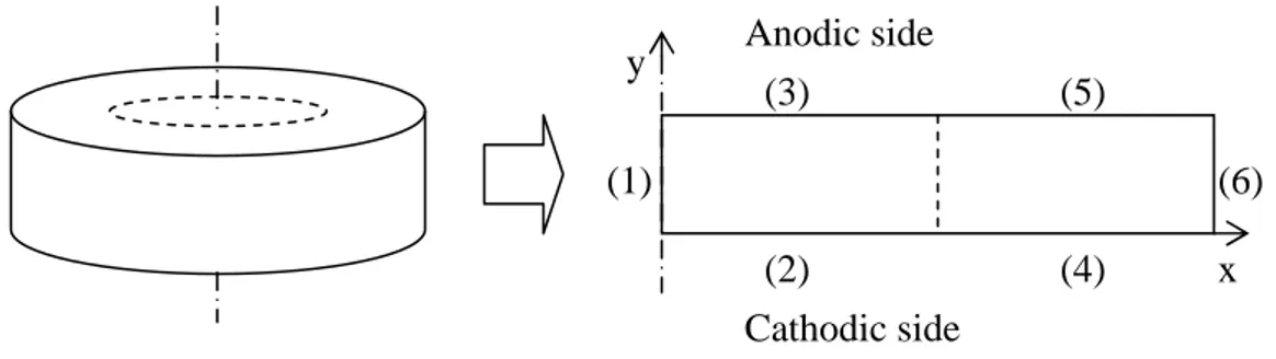
The system described in the previous paragraph can not be solved without consistent boundary conditions. In particular, according to the fact that the geometry of the CM is cylindrical, we use the axial symmetry of the domain to simplify the resolution of the system. It means that we reduce the problem in two spatial dimensions instead of three, i.e. spatial coordinates will be only the radial coordinate x and the axial one y (fig. V.1; note that dotted lines represent the projection of the electrodes).

fig. V.1 – Reduction of the model of the CM from 3D to axial symmetric 2D.

The modelling in axial symmetric 2D implies that the divergence of fluxes must take into account the increase or radius, for example, (eq. V.2.1) becomes in explicit form:

(1) (2) (3) (4) (5) (6) x y Anodic side Cathodic side

t F a c F i y N x N x N 0 v dl dl v TPB s y H x H x H ∂ ∂ − −         ∂ ∂ + + ∂ ∂ − = + + + λ η (eq. V.3.1) ∇⋅N_H+

in which NxH+ and NyH+ represent the first and the second component of the flux of

protons, i.e. by using (eq. V.2.6):

y V F x V F N N N PCP app PCP PCP app PCP y H x H H ∂ ∂ − ∂ ∂ − = = + + + σ σ (eq. V.3.2)

Thus, according to fig. V.1, boundary conditions are expressed for the 2D model (but they are easily convertible in 3D) for dynamic conditions as:

( )

(

)

( )

(

)

( )

(

)

( )

( )

( )

φ

We impose either values of variables (e.g. in (sys. V.3.2) VACP = 0) or normal fluxes

(e.g. in (sys. V.3.1) nˆ N 0

H =

⋅ + ); with nˆ we mean the normal unitary vector that exits

from the face (for example, for boundary (1) the direction of nˆ is from right to left).

Some explanations concerning (sys. V.3.1-6) are needed:

• in (sys. V.3.2) the condition VACP = 0 is a reference for electric potential in ACP;

electric potentials are always based on a reference, we choose 0V for ACP at the interface with anionic electrolyte;

• in (sys. V.3.3) we set the electric potential of PCP at the interface with protonic electrolyte. In dynamic conditions, i.e. when we simulate a measurement of impedance, a sinusoidal input is assigned; f is the frequency of the oscillation3. In steady-state simulations the applied overpotential is a constant value. In both cases the overpotential of the whole CM

η

(

)

∆

η

i.e. the difference between the equilibrium potential referred to external condition and the difference of potential between ACP at the interface with anionic electrolyte and PCP at the interface with protonic electrolyte (see also (eq. I.3.8) in par. I.3). According to the reference VACP = 0 and to (eq. V.2.13) that yields ∆Veq,ex = 0, VPCP at boundary (3) is equal to the whole overpotential applied

η

(that can be constant or variable with time).

Note that (eq. V.3.3) is consistent with equilibrium condition and kinetics of water recombination: when

η

pw = pwex (equilibrium into gas phase), in each point

η

occur. We could say that (eq. V.3.3) as it is written is a direct consequence of the way that we use to calculate ∆Veq as described in par. IV.1, i.e. referring all electric potentials to external conditions.

Concluding: we said in par. II.1 that ACP and PCP at equilibrium have different absolute potentials, then in par. IV.1 we demonstrated that we could work with relative (i.e. not absolute) potentials; we can say that we set an arbitrary reference for VACP in (sys. V.3.2) and a reference for VPCP as regards the water

recombination reaction when we define equilibrium potential as in (eq. V.2.13). All these relative quantities are coherent one other and with the whole cell;

• in (sys. V.3.3) for adsorbed water in PCP a flux from CM to anode is considered if there is a difference of concentration of water in PCP between the CM-protonic electrolyte interface and protonic electrolyte-anode interface. In particular, we consider as a simplified condition that the concentration of water at the anodic side is in equilibrium with partial pressure of water of the gas supplied at the anode, i.e.:

(

)

δ

by using (eq. IV.3.15) and remembering the relationship between cOH and Cw,PCP,

i.e. combining (eq. IV.3.1) with (eq. IV.3.10). Under this assumption, the flux is expressed with the Fick law with a mean diffusion coefficient calculated as:

2 D D D an PCP , w PCP , w PCP , w + = (eq. V.3.5)

where Danw,PCP is the diffusion coefficient for water transport in PCP calculated at

the anodic side with concentration of water adsorbed (i.e. protonic defects) equal to the result of (eq. V.3.4). Dw,PCP is the diffusion coefficient inside the CM,

calculated in the same manner in each point of the boundary (3) according to the local concentration of water adsorbed (see sec. V.4.5, in particular (eq. V.4.6));

• in (sys. V.3.5) we do not consider a flux of adsorbed water as in (sys. V.3.3) because the pipe that supplies wet hydrogen at the anode covers the upper surface of the protonic electrolyte (see par. II.8). Note that, if the pipe had a very little thickness, if it was of the same diameter of the CM we should consider a flux proportional to the difference Cw,PCP – Canw,PCP as done before, if it was of the

same diameter of the electrode the flux would be proportional to Cw,PCP – Cexw,PCP

(with Cexw,PCP calculated by using (eq. V.3.4) but with pwex instead of pwan)

because the upper surface of the protonic electrolyte would be in contact with external atmosphere4. Anyway, we neglect the flow of adsorbed water between protonic electrolyte and external atmosphere in the radial direction because the thickness of protonic electrolyte tPCE is very small if compared with its radius. So,

the boundary condition used in our simulation for water adsorbed in PCP is a simplified but reasonable condition. Fig. V.2. schematizes the last two boundary conditions for a generic case. We repeat that in our simulations, only the flux towards and through the anode (i.e. the first on the left) is considered because the thickness of the pipe is enough to cover the external upper surface of protonic electrolyte and we neglect the flux in radial direction;

fig. V.2 – Schematization of boundary conditions in (3) and (5) for water adsorbed in PCP for a generic case.

4 _{These are the two limit cases, we could also consider a pipe with a radius between the radius of the CM}

rCM and the radius of electrodes rE. In this generic case boundary (5) should be separated into two parts:

the more internal one would be connected with anode, the other one with external atmosphere. pwan

pwex

always neglected

• it is important to note that, because the thickness of protonic electrolyte tPCE is

very small if compared with radii of CM rCM and electrodes rE, we use the

projection of electrodes to impose boundary conditions to the CM. It means that we neglect the possibility that flows (of charges or of water adsorbed) exit in the radial direction from the ideal cylinder with the base equal to the base of electrodes. In particular, we are saying that the radial extension of boundaries (2) and (3) could be bigger in spite of the extension of (4) and (5) but we are neglecting this effect5;

• in (sys. V.3.6) we are considering constant conditions for the outer atmosphere (i.e. xwex and Pex are constants), so we are assuming that the production of water

in the CM does not affect external conditions because negligible if compared with the flow of wet nitrogen out of the CM. This is a reasonable assumption if compared with experimental conditions. We could repeat the same thing for the partial pressure of water at the anode.

Only for dynamic simulations initial conditions (i.e. at t = 0) are needed too. We set in the whole domain:

(

)

(

)

(

)

(

)

(

)

It is important to note that initial condition is coincident with an equilibrium condition only if the partial pressure of water at the anode pwan is equal to the partial pressure of

water in the outer atmosphere pwex. If no overpotential

η

driving force for the transport of water in PCP through the protonic electrolyte, the CM is characterized by uniform conditions. If pwan ≠ pwex, a net flow of water goes from CM

to anode or vice versa, so initial condition is not representative of equilibrium. Anyway, steady-state condition will be reached but in that situation variables as Cw,PCP, xw and P

will not be uniform in the CM; for example, if pwan < pwex in steady-state conditions

there is a flow of water from CM to anode through the protonic electrolyte: in this

5 _{If we modeled the whole cell this problem would not exist, it is a limit of the fact that we are modelling}

only the CM. However, the assumption that we are doing should be reasonable because tPCE/rE << 1. This

situation it is reasonable that P < Pex and xw < xwex inside the CM (in order to create the

flow of water) and also that Cw,PCP < Cexw,PCP. Some consequences of this effect will be

treated in par. V.7.

V.4 – Working conditions and estimation of parameters

In this paragraph we will show all the parameters (physical, geometrical, etc.), working conditions and design variables that the model of the CM needs. So, this paragraph is the “input” for the resolution of the system of equations as described in par. V.2.

V.4.1 – Geometric variables

They are the thickness of the central membrane (tCM) and of electrolytes (tACE and tPCE

for anionic and protonic electrolytes), the radius of the electrodes (rE) and of the CM

and electrolytes (rCM) that are the same (see par. II.8). They are design variables. In

details:

• thickness of the CM (tCM): we set 400µm by default because close to the

thickness normally used now in the preparation of IDEAL-Cells (about 500µm, Thorel et al., 2009). It can vary in design analysis (sec. VI.5.4) within a reasonable range (40-650µm);

• thicknesses of electrolytes (tACE and tPCE): only the thickness of protonic

electrolyte tPCE affects the results of the model of the CM because it is linked with

the flow of adsorbed water through the protonic electrolyte from anode to CM or vice versa. By default 50µm is used but a design analysis will be performed in the range 50-500µm (sec. VI.5.5);

• radius of electrodes (rE): we use 5mm according to some existing samples of

IDEAL-Cell. Other values are used in validation (par. VI.2) to match the exact geometry of the cell which we refer;

• radius of CM (rCM): by default 10mm is used according to some existing samples

of IDEAL-Cell; in validation (par. VI.2) rCM will be equal to the exact radius of

the cell analyzed. A design analysis will be performed in sec. VI.5.3 in the range 7.5-10mm.

V.4.2 – Morphological parameters

Morphological parameters such as the length of TPB per unit volume (λvTPB), the

contact area between connected particles (adlv), the total surface area exposed by PCP to

gas phase per unit volume (avPCP) and the mean diameter of pores (dp) enter in the

model of the CM or in submodels. They are functions of the granulometric distributions of particles for each phase (proton-conducting, anion-conducting and pore formers) and of compositions; their estimation is made by using chap. III.

We reproduce the granulometric distribution of particles in order to achieve a good agreement with suppliers data (Marion Technologies for BCY15, i.e. the PCP, and YDC15, i.e. the ACP)6, in particular we use:

m 126 . 0 r m 108 . 0 r m 09 . 0 r m 072 . 0 r m 054 . 0 r 5 PCP 4 PCP 3 PCP 2 PCP 1 PCP

µ

µ

µ

µ

µ

ψ

ψ

ψ

ψ

ψ

ψ

ψ

ψ

ψ

ψ

µ

µ

µ

µ

µ

ψ

ψ

ψ

ψ

ψ

ψ

ψ

ψ

ψ

ψ

in which ψPCP, ψACP and ψf are the volume fractions of PCP, ACP and pore formers

before sintering (voids excluded).

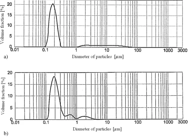
Thus, we approximate the real granulometric distribution of powders, as reported in fig. V.3 for PCP and ACP, as better as possible. The granulometric distribution of pore

6

We remember here that BCY15 means BaCeO3 doped with 15% of Y (i.e. BaCe0.85Y0.15O2.925), YDC15

formers in (sys. V.4.3) is a guess based on images of the central membrane after sintering made with the electronic microscope, there is not a size distribution of pore formers (polyvinyl butiral)7.

fig. V.3 – Particle size distributions of a) PCP and b) ACP as given by the supplier (Marion Technologies).

It is important to emphasize that because the mean particle size of powders is the same (i.e. rPCP3 = rACP3 = rf3) it implies that:

1. it is reasonable to assume an initial porosity before sintering φg = 0.36 equal to a

random mixture of monosized particles (see sec. III.5.1);

2. it is possible to use our model of estimation of apparent conductivity as described in sec. III.4.5.

In particular, we never change the parameters φg = 0.36 (i.e. porosity before sintering)

and θ = 15° (mean angle of contact). We will do a design analysis on the final porosity

7 _{It s important to remember that polyvinyl butiral has a quite spherical shape before sintering and leaves}

hollow sites of the same form: this feature allows us to use the percolation theory in par. III.2 and par. III.5. Remember also that this kind of pore formers creates a fine and homogeneous porosity that is useful for the global performance of the CM (on the other hand, a few big pores are useless for gas transport).

a)

of the CM φgfin that will vary from 40 to 50%8 in sec. VI.5.1; by default, φgfin = 0.4 is

used. Then, we always use ψPCPas = 0.5, i.e. whatever is the final porosity the

composition after sintering is 50% PCP and 50% ACP in volume fraction for solid phase, according to some existing samples of IDEAL-Cell.

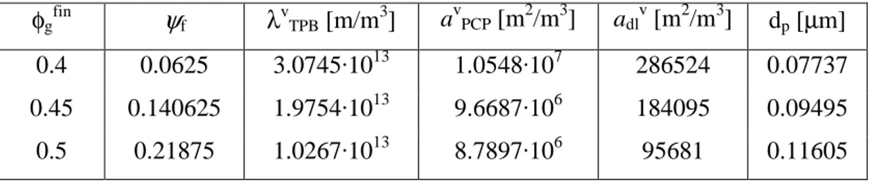
Tab. V.1 resumes all the morphological parameters (that we directly use in the model) at several final porosities for ψPCPas = 0.5.

φgfin ψf λvTPB [m/m3] a v PCP [m2/m3] adlv [m2/m3] dp [µm] 0.4 0.0625 3.0745·1013 1.0548·107 286524 0.07737 0.45 0.140625 1.9754·1013 9.6687·106 184095 0.09495 0.5 0.21875 1.0267·1013 8.7897·106 95681 0.11605

tab. V.1 – Morphological parameters at several porosities.

V.4.3 – Physical parameters for gas phase

They are the molar weights of gaseous substances (Mw and MB), the dynamic viscosity

of gas mixture (µ) and of gases (µw and µB), the ordinary diffusion coefficient (DwB) and

the mean diameters of gaseous substances (dm,w and dm,B); they are all referred to gas

phase. In all our simulations the second component in gas phase is nitrogen (i.e. B means nitrogen) as in experimental conditions (par. II.8). In details:

• molar weights (Mw and MB): we use for water Mw = 18·10-3kg/mol and for

nitrogen MB = 28·10-3kg/mol;

• viscosities: we use the Herning and Zipperer method (Shan et al., 2001) to estimate the viscosity of the gas mixture starting from the viscosities of pure gases and composition:

(

)

(

)

8 _{As explained in par. III.5, higher values of porosity could invalidate the assumption that pore formers}

leave holes of the same shape and dimension of original particles without distortion of the structure. It is a limit of our model of description of morphology.

According to Todd and Young (2002) this method gives mean deviations in the order of -2% between predictions and measurements for gas mixtures and conditions normally used in SOFCs9.

For the estimation of dynamic viscosities of pure substances µw and µB we use the

relationship suggested by Todd and Young (2002):

[

]

in which t = T·10-3K and parameters bj,j are reported in tab. V.2; µi are in SI. Note

that we neglect any dependence of viscosity on pressure because for water and nitrogen in our working conditions (i.e. pressure less that 5atm and temperature above 873K) dynamic viscosity is independent on pressure (Bird et al., 1960).

b0,i b1,i b2,i b3,i b4,i b5,i b6,i

w -6.7541 244.93 419.50 -522.38 348.12 -126.96 19.591

B 1.2719 771.45 -809.20 832.47 -553.93 206.15 -32.430

tab. V.2 – Parameters of water and nitrogen for (eq. V.4.2).

• ordinary diffusion coefficient (DwB): Todd and Young (2002) suggest to use

Fuller correlation: 2 3 1 3 1 5 . 0 B 3 w 3 75 . 1 wB 7 . 12 9 . 17 P M 10 M 10 T 01013 . 0 D     ₊ ⋅       + ⋅ = − − (eq. V.4.3)

as in Perry and Green (1997)10; all the quantities are in SI (T in K in particular);

• mean diameters of gaseous molecules (dm,w and dm,B): they are used only in (eq.

IV.2.13) to check the region of flow, their role is really marginal (they are not key

9 _{According to Todd and Young (2002), Reichenberg method is the best one; we have chosen Herning}

and Zipperer method because it has a simple expression and its accuracy is enough for our purposes.

10 _{Note that there is a mistake in equation (2-152) of Perry and Green (1997): the coefficient that shall be}

used is 0.01013 instead of 0.1013, just compare the formula with one reported in Todd and Young (2002). Anyway, (eq. V.4.3) is correct.

parameters). We use for water dm,w = 0.282nm (Franks, 2000) and for nitrogen

dm,B = 0.368nm (Bird et al., 1960)11.

V.4.4 – Ohmic parameters

They are the conductivities of pure compact solid phases (σACP and σPCPsat) and the

way that we use to estimate apparent conductivities. We have already said (sec. III.4.3 and par. III.8) that we use as conductivity of pure material the conductivity of the sintered dense material in order to consider in one parameter both intra-particles and inter-particles contributions; this is in agreement with our method to estimate apparent conductivity (par. III.4).

We assume no-mixed conduction (par. II.1), so the conductivity of ACP (i.e. YDC15) is referred to the transport of only oxygen ions and of PCP (i.e. BCY15) to only protons12. Under these considerations, we use values of conductivity as reported in tab. V.3, i.e. taken from Van herle et al. (1996) for YDC15 and from Katahira et al. (2000) for BCY1513; these values are quite in agreement with internal measurements of conductivity (Vladikova, 2009), especially for ACP. It shall be noted that Katahira et al. (2000) report measurements at partial pressure of water equal to 1700Pa; we extrapolate

σPCPsat by using (eq. IV.4.4) and (eq. IV.3.15).

T [°C] σACP [S/m] σPCPsat [S/m]

600 1.5488 1.9844

650 2.5704 3.3970

700 3.0819 5.8272

tab. V.3 – Conductivities of ACP (i.e. YDC15) and PCP (i.e. BCY15) as reported by Van herle et al. (1996) and Katahira et al. (2000).

Remember that conductivity of ACP is constant (it is dependent only on temperature) while the conductivity of PCP depends also on the local concentration of protonic defects as in (eq. IV.4.4).

11 _{Actually, d}

m,B is taken equal to Lennard-Jones diameter: it is not the same thing but it is a reasonable

approximation.

12

In particular, BCY15 and other PCPs are mixed conductors of protons and oxygen ions (Coors, 2007; Suksamai and Metcalfe, 2007). When partial pressure of oxygen approaches zero, as it happens at the anode and in the CM of the IDEAL-Cell where there is not molecular oxygen, the anionic conductivity of PCP seems to disappear; so, it is reasonable to neglect the anionic conductivity of PCP in our case.

13

Actually, Katahira et al. (2000) give values for BCY10, but according with Kreuer (2003) the conductivity of BCY15 is very close to the conductivity of BCY10.

The values of apparent conductivities in the CM are calculated as:       ⋅ = iCP app iCP iCP app iCP

σ

σ

σ

σ

in which the correction factor is estimated according to (eq. III.4.12). In particular, when the composition after sintering is 50% ACP and 50% PCP, we get correction factors equal to 2.265·10-2, 1.375·10-2 and 7.323·10-3 respectively for final porosity of 0.4, 0.45 and 0.5. It is possible to use (eq. III.4.12) because particles are quite monosized as mentioned in sec. V.4.2. A sensitivity analysis will be done on these correctors due to the uncertainties of their estimation (sec. VI.4.3).

V.4.5 – Parameters of transport and adsorption of water in PCP

They are the density of perovskite-cells per unit volume (δ), the diffusion coefficient for water in PCP (Dw,PCP) and the thermodynamic constant of adsorption (K). In details:

• density of perovskite-cells per unit volume (δ): it is a property of PCP and allows us to convert concentration of protonic defects (i.e. of water adsorbed) COH

expressed in mol/m3 into concentration per unit of cell cOH as mol/mol cell. δ

represents the number of moles of perovskite-cells per cubic meter, i.e. it is possible to estimate it as:

PCP PCP M d =

δ

in which dPCP is the density of pure compact PCP, equal to 6210kg/m3 for BCY15

in the range 600-700°C (Presto, 2009), and MPCP is the molar weight of the

perovskite-cell that constitutes the material, equal to 0.316934kg/mol14 according to the supplier (i.e. Marion Technologies). So, in our case δ = 19594mol/m3;

• diffusion coefficient for water in PCP (Dw,PCP): according to Coors (2007), it is

not constant but it depends on the concentration of protonic defects as:

14

It is the molar weight of BCY15 that is represented by the chemical formula Ba0.98Ce0.87Y0.15O2.945 as

s VO OH s OH OH s VO s OH OH PCP , w D S c 1 2 D S c D D S c 2 D       − +       − = (eq. V.4.6)

in which DsOH and DsVO are the self-diffusivities of protonic defects and oxygen

ion vacancies, i.e. a measure of the rate of exchange of a protonic defect (or of a vacancy) with another one. The self-diffusivities are quite independent from cOH,

so they are properties of the material estimated as (Coors, 2007):

        − ⋅ = − T R 33765 exp 10 74 . 7 D g 8 s OH (eq. V.4.7)         − ⋅ = − T R 53060 exp 10 63 . 3 D g 7 s VO (eq. V.4.8)

These values (in SI) are for BCY10, we assume that they are valid also for BCY15.

Suksamai and Metcalfe (2007) found values of Dw,PCP about 10 times higher: we

use (eq. V.4.6-8) by default, then we will do a sensitivity analysis on this parameter as self-diffusivities were up to 10 times higher (sec. VI.4.4).

In the model of CM we must use an apparent diffusivity for water in PCP; it is possible to estimate it as:

      ⋅ = PCP app PCP PCP , w app PCP , w D D

σ

σ

We use the same correction factor used for conductivity because Ohm law of conduction and Fick law of diffusion follow the same relationship in which flux (current or mass flux) is proportional to a gradient of driving force (electric potential or concentration) by a conduction factor (conductivity or diffusivity). So, because the relationship and the phase (i.e. the domain) are the same, also the way to correct conduction factors is the same;

• thermodynamic constant of adsorption (K): according to Kreuer (2003) it is equal to:

        ₋ − = − T R S T H exp 10 K g 0 ads 0 ads 5 ∆ ∆ (eq. V.4.10)

in which ∆H0ads = -163’000J/mol and ∆S0ads = -167.9J/(mol·K). These values (in

SI) are for BCY10, we assume the same values for BCY15.

V.4.6 – Kinetic parameters

They are the exchange current per unit of length of TPB (i0), the kinetic constant of

water adsorption (kd) and the capacitance of the double layer (cdl)15. They are unknown

parameters for our system, specific experiments must be performed for their evaluation. For our simulations we use:

• exchange current per unit of length of TPB (i0): from validation (par. VI.2) we

estimate 8·10-9A/m at 873K from the best fitting of experimental polarization curves made on existing samples. As explained in sec. VI.4.1, i0 could be

reasonably higher. A sensitivity analysis will be performed because it is a key parameter;

• kinetic constant of water adsorption (kd): it is an unknown parameter. We set by

default 5·10-13mol/(m2·Pa·s) at 873K (it is a guess) and a sensitivity analysis on a wide range will be performed (sec. VI.4.2);

• capacitance of the double layer (cdl): it is an unknown parameter that has a role in

dynamic simulations. It can be estimated from impedance curves. We use by default cdl = 5·10-2C/(m2·V) at 873K, it is a guess16.

V.4.7 – Working conditions

They are the temperature (T), the total pressure out of the CM (Pex), the molar fraction of water out of the CM (xwex), the partial pressure of water at the anode (pwan) and the

overpotential applied to the CM (ηCM). In details:

• temperature (T): we assume isothermal conditions inside and outside the cell neglecting in this way the heat fluxes related to reaction, adsorption and transports; so T is the temperature of gas and solid phases in the CM. By default

15 _{We consider c}

dl as a kinetic parameter because it affects the rate of charge/discharge of double layer at

ACP-PCP interface.

16

In particular, we set this value to have the maximum of the first arc in the impedance curve of the base-case corresponding to 50Hz, it is an arbitrary choice (see also par. VI.6).

873K (600°C) is used because it is the temperature normally used in experiments on samples of the cell;

• total pressure out of the CM (Pex): we set by default 1.013·105Pa (1atm) because it is the pressure used in experiments;

• molar fraction of water out of the CM (xwex): by default we use xwex = 0.05. At the

moment, in experiments the molar fraction of water is very low, in the order of hundreds of ppmV. So, xwex = 0.05 is our suggestion in order to reach stable

results (e.g. a stable OCV or polarization curves): if xwex is very low the

production of water due to the passage of current through the cell affects the molar fraction of water out of the CM, i.e. results from experiments will be unstable due to this reason. Therefore if we use wet nitrogen in the third chamber (see par. II.8) the amount of water produced by the cell is negligible if the flow of nitrogen is high, so it is reasonable to assume xwex constant and equal to the

humidity of nitrogen (i.e. it is a stable boundary condition).

When the cell will be used as an energy supplier, the molar fraction of water out of the CM will be due to a balance between the electrochemical production and the evacuation from the third chamber, in this condition xwex could be very high.

Anyway, this working configuration is still far, so we have chosen to perform simulations close to actual and future experimental conditions. The effects of the variation of xwex will be shown in sec. VI.4.5;

• partial pressure of water at the anode (pwan): as explained in par. II.2 and par. II.8,

at the anode wet hydrogen is fed to increase the conductivity of the proton-conducting material used in anode, electrolyte and CM. We set pwan = 3039Pa as

the result of 3% of water in a flow of hydrogen at 1atm as used in experimental conditions. This parameter, despite not strictly associated at the CM, plays a role (as also the thickness of protonic electrolyte) because connected with the exchange of water between CM and anode through the transport in PCP;

• overpotential applied to the CM (ηCM): it is the input17 that generates the passage

of current through the CM, when no overpotential is applied there is not a passage of current and the cell is in equilibrium. By default ηCM = 0.3V is used as

boundary condition in (sys. V.3.3) but in several simulations (e.g. in polarization curves) it is a working variable.

17 _{Generally speaking, in experiments and in the model we can impose an overpotential and}

measure/calculate the current passed or it is possible to impose a flow of current and measure/calculate the overpotential generated to allow this passage.

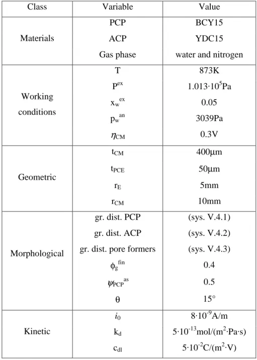
We resume in tab. V.4 all the conditions and kinetic parameters (that are guesses except i0) of the base-case (i.e. when in chap. VI we will say base-case we will refer to

these conditions that are the real starting input parameters of the model).

Class Variable Value

PCP BCY15

ACP YDC15

Materials

Gas phase water and nitrogen

T 873K Pex 1.013·105Pa xwex 0.05 pwan 3039Pa Working conditions ηCM 0.3V tCM 400µm tPCE 50µm rE 5mm Geometric rCM 10mm gr. dist. PCP (sys. V.4.1)

gr. dist. ACP (sys. V.4.2)

gr. dist. pore formers (sys. V.4.3)

φgfin 0.4 ψPCPas 0.5 Morphological θ 15° i0 8·10-9A/m kd 5·10-13mol/(m2·Pa·s) Kinetic cdl 5·10-2C/(m2·V)

tab. V.4 – Conditions and kinetic parameters used in base-case.

V.5 – Energy balance

The energy balance of the CM is an equation of conservation that we do not need to solve the problem. The system (eq. V.2.1-5) is closed (i.e. it is possible to solve it

because there are 5 variables and 5 balances); the energy balance will be an identity. This happens because we assume uniform temperature in the whole cell (see par. V.1), i.e. we are neglecting heat effects due to transports or reactions. The energy balance would be an equation that we should consider coupled with the system (eq. V.2.1-5) if we considered heat effects. In such case temperature would be a dependent scalar variable, function of spatial position (i.e. x and y) and time, so we would have 6 variables and 6 equations of conservation18.

Despite the energy balance is an identity, it is interesting to show it. In particular, we apply the energy balance in steady-state conditions when a positive overpotential ηCM is

applied to the central membrane. We use an approach that we could call the “energy luggage”: protons and oxygen ions are considered as charges, so the balance is made per unit of charge (i.e. in terms of electric potential).

The energy applied to a unit charge at the protonic electrolyte-CM interface is equal to

ηCM. The charge spends its luggage across the CM to win ohmic resistances in PCP till

the reaction site (wherever it is), the activation resistances to react, the ohmic resistances in ACP to go from reaction site to anionic electrolyte and then to evacuate water produced. For simplicity, we assume that water is evacuated only towards the outer atmosphere, i.e. we are neglecting the transport of adsorbed water in PCP and considering only the evacuation by gas phase. So, this means that the energy equation (that is a balance of energy lost across the CM), expressed per unit of charge is equal to:

evac , g ohm , ACP ohm , PCP CM η η η η η = + + + (eq. V.5.1)

Each term, according to the explanation and the representation in fig. V.4, is calculated as:

( )

(

)

η

( )

18 _{We are talking about a simplified situation in which temperature is the same for ACP, PCP and gas}

phase; a more general model should consider three different temperatures (i.e. one for each phase) and so an energy balance for each phase.

      = _ex w w g evac , g p p ln F 2 T R

η

fig. V.4 – Energy luggage: schematic representation of the losses of energy in CM.

Some explanations are needed:

• (eq. V.5.2) represents the loss of electric potential due to the transport of the charge in PCP, i.e. it is the difference between the potential at the CM-protonic electrolyte interface and the electric potential in PCP at the reaction site (i.e. the final point); (eq. V.5.4) is the same for ohmic losses in ACP from reaction site to anionic electrolyte;

• (eq. V.5.3) is the definition of the overpotential as (eq. V.2.12) in which (eq. V.2.13) is substituted; remember that activation overpotential is the energy lost so that the electrochemical reaction can proceed at a finite rate (see par. I.3);

• (eq. V.5.5) can be explained by using the concept of exergy: exergy is the maximum work that a system can give. In our case, water at pressure pw goes in

an ambient with a lower pressure pwex: the maximum work that water could do is

equal to the physical exergy Exph, equal to (Douvartzides et al., 2003):

(

)

(

)

_∫

_∫

in which h is the enthalpy, s the entropy and cp the specific heat at constant

pressure19. With the assumption of uniform temperature (T = Tex) and remembering that a molecule of water is related with 2 charges, (eq. V.5.6) gives (eq. V.5.5) if referred per unit of charge. So, ηg,evac represents the maximum work

19 _{Note that the calculation of h and s is for an ideal gas, i.e. according to point 8 in par. V.1.} ηCM ηPCP,ohm ηACP,ohm ηg,evac η 0 tCM

that water inside CM could do but it is lost in the resistances of the transport through the porous structure of the CM20.

If we put (eq. V.5.2-5) into (eq. V.5.1) we obtain the definition of overpotential applied to the central membrane ηCM as expressed in (eq. V.3.3), i.e. we obtain an

identity (not useful for the resolution of the problem).

Thus, we have shown by a simple approach21 that we do not need an energy balance to solve the problem, so the solution relative to the resolution of (eq. V.2.1-5) has itself the information of the energy balance. It is interesting to note that only η is the contribution of the energy luggage that the system spends for the reaction, the other 3 terms are losses. In other words, activation overpotential η is the energy that the system must necessarily spend so that the electrochemical reaction proceeds with a finite rate. For the design of the CM it is important that in each point η approaches ηCM, i.e.

minimizing ohmic losses and losses relative to water evacuation, in order to achieve the maximum energetic efficiency. On the other hand, in a not optimized CM the difference between ηCM and η represents in each point the contribution of energy that is lost and it

is useless for the reaction.

The last consideration is important because it is useful to define some limit cases: 1. when in the whole CM the ratio η/ηCM is close to 1 the energy is spent principally

for the occurring of the reaction: we call this situation kinetic regime. In this case, the kinetics of water recombination reaction is the rate determining step of the process;

2. when in the whole CM the ratio (ηPCP,ohm+ηACP,ohm)/ηCM is close to 1 the energy is

spent principally in the charge transport: we call this situation ohmic regime. In this case, the transport of charges inside the CM is the rate determining step of the process;

3. when in the whole CM the ratio (ηg,evac)/ηCM is close to 1 the energy is spent

principally in the transport of water in gas phase: we call this situation gas transport regime. In this case, the transport of water in gas phase through the CM is the rate determining step of the process.

20

Note that we have used the exergy because the luggage ηCM is a “coherent” form of energy as the other

quantities in (eq. V.5.2-4), so a “coherent” form of energy is needed also to express ηg,evac.

21 _{It is possible to write an energy balance with the classic thermodynamic approach, i.e. considering a}

volume of control inside the CM and applying the conservation of energy considering energetic contributions of mass fluxes, current (i.e. electric power) and heat fluxes (equal to zero if temperature is uniform): conclusions and results would be the same.

Also a combination of regimes is possible, for example an ohmic-gas transport regime is representative of a situation in which kinetics of water recombination is easy but charge and gas transports meet high and comparable resistances. The knowledge of the regime is very important in the design and to predict and explain the behaviour of the CM when one or more parameters vary.

V.6 – Performance indexes

The solution of the system (eq. V.2.1-5) gives the dependence of the 5 variables as a function of spatial coordinates and time (e.g. VACP(x,y,t)). In order to characterize the

global performance of the CM, we calculate from the solution some performance indexes.

The first performance index is the density of current that passes through the CM (that is linked to the production of water); it is straightforward to understand that it is important to reach the highest values of density of current as possible because it means that the cell is able to supply high current.

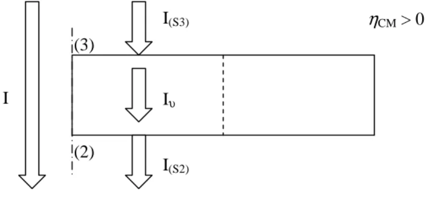
The density of current i is defined as the ratio of the current that flows through the CM and the nominal section of the electrodes, i.e. it means that the current I is normalized at the section of electrodes equal to πrE2. Under steady-state conditions with ηCM > 0, the

current exchanged in water recombination reaction Iυ is equal to the current that enters in the CM from protonic electrolyte IS(3) (as flow of protons) and to the current that exits

from the CM towards the anionic electrolyte IS(2) (as flow of oxygen ions):

state steady in I I I I = _υ = _S(3) = _S(2) − (eq. V.6.1) in which:

∫

∫

(

)

∫

Thus, Iυ is calculated as integral of the current exchanged in the water recombination reaction in the volume of the CM υ, I(S3) is calculated as surface integral on boundary

(3) of the normal flux of protons multiplied by F (i.e. the charge of 1mol of protons), I(S2) is calculated as surface integral on boundary (2) of the normal flux of oxygen ions

multiplied by –2F (i.e. the charge of 1mol of oxygen ions). Note that is, NH+ and NO-2

are calculated by (eq. V.2.11), (eq. V.2.6) and (eq. V.2.7). Obviously, (eq. V.6.1-4) are still valid for ηCM < 0, in such case currents are negative (i.e. current flows in the

opposite direction). Fig. V.5 schematizes the concepts explained above.

fig. V.5 – Schematic representation of the calculus of currents.

In steady-state conditions the density of current i is calculated as:

state steady in r I r I r I i r I i ₂ E ) 2 ( S 2 E ) 3 ( S 2 E 2 E − = = = ⇒ =

π

π

π

π

In dynamic conditions (i.e. in impedance measurements), I_υ as in (eq. V.6.2) is not representative of the current I that passes through the CM because a fraction of I is reserved to capacitive effects, i.e. to charge/discharge of the double layers represented by ACP-PCP interfaces (see par. II.2). So, the density of current must be calculated as:

conditions dynamic in r I r I i r I i ₂ E ) 2 ( S 2 E ) 3 ( S 2 E

π

π

π

that is the generalization of (eq. V.6.5). It is important to note that i is an incomplete information without the knowledge of the overpotential applied to the CM.

22 _{In general, in steady-state conditions we calculate i by using I}

υ because it is more accurate. (2) (3) I(S3) I_υ I(S2) I ηCM > 0

Another important index is the polarization resistance Rp, defined as: i R CM p η = (eq. V.6.7)

where i is the density of current as explained before and ηCM is the overpotential applied

to the CM in steady-state conditions or the amplitude of the overpotential imposed in impedance measurements (see (sys. V.3.3)). Polarization resistance is an indirect measurement of the efficiency of the CM, the aim of the design is to reduce Rp as much

as possible (i.e. to obtain high density of current at low overpotential).

Concerning the gas phase, it is important to know if water evacuation is simple or not, in particular, in several conditions it is interesting to know if water is mainly evacuated by convection or diffusion23. According to Bird et al. (1960), fluxes into gas phase can be expressed as: g , w m g w g , w v J T R P x N = + (eq. V.6.8)

(

)

in which vm is the molar average velocity, Jw,g and JB,g are respectively the diffusive

fluxes of water and nitrogen and P/(RgT) is the molar concentration into gas phase

according to the ideal gas model. In particular, diffusive fluxes are equal and opposite:

g , B g , w J J =− (eq. V.6.10)

so, by combining (eq. V.6.8-10), the molar average velocity is calculated as:

(

)

23 _{This information is important during the optimization of the central membrane because we will put into}

effect modifications on the geometry and morphology of the CM in order to maximize water evacuation; this is possible only if we know the kind of transport that characterizes gas phase.

in which Nw,g and NB,g are calculated by using (eq. V.2.9-10). In this way, with (eq.

V.6.8) the diffusive flux of water in gas phase is determined as:

m g w g , w g , w v T R P x N J = − (eq. V.6.12)

In steady-state conditions, the ratio between the module of diffusive and total flux of water, i.e. |Jw,g|/|Nw,g|, is a way to discriminate if the transport of water is mainly

diffusive or convective. Note that when ηCM > 0 water exits from the CM in radial

direction, so Nw,g is a vector oriented from the center of the membrane to the outside;

then, also the diffusive term Jw,g has the same direction while nitrogen is stagnant: this

means that the module of Jw,g is lesser than the module of Nw,g and the direction is quite

the same, so the comparison is possible. In a similar way, it could be possible to compare only the radial components of the fluxes, i.e. Jxw,g and Nxw,g. For ηCM < 0 the

considerations are the same, only the direction of flows changes. Fig. V.6 represents a schematization of these concepts for ηCM > 0 when a) the molar fraction of water xw is

low or b) close to 1 (for simplicity, only radial components of fluxes are represented).

fig. V.6 – Schematization of fluxes of water and nitrogen in gas phase for ηCM > 0 for:

a) xw ≈ 0; b) xw ≈ 1.

In steady-state conditions, assuming that the overpotential applied to the CM is positive (but the same considerations could be done also for ηCM < 0), water produced

Nw,g m g w v T R P x Jw,g JB,g

(

)

(

)

by the reaction Fw(r) must be equal to the sum of water desorbed into outer atmosphere

through boundary (6) Fw(des), water evacuated into the outer atmosphere by gas phase

through boundary (6) Fw(g) and towards the anode across the protonic electrolyte

through boundary (3) Fw(PCE) (see fig. V.1 to visualize the boundaries):

) PCE ( w ) g ( w ) des ( w ) r ( w F F F F = + + (eq. V.6.13)

The first member of (eq. V.6.13) represents the global amount of water that enters in the CM, the second member the global amount that exits from the CM. Each term is calculated as:

∫

υ

λ

∫

∫

∫

Note that the quantities described above have a sign, for example Fw(des) is positive if

water exits from the CM to the outer atmosphere and vice versa or Fw(PCE) is positive if

water goes from CM to the anode and vice versa.

These quantities are interesting because they say how water is evacuated from the CM. In particular, in the base-case (tab. V.4) partial pressure of water inside the CM is bigger than partial pressure of water at the anodic side, so Fw(PCE) is positive. Thus, the

ratio (Fw(PCE)+Fw(des))/Fw(r) is representative of the fraction of water evacuated in

adsorbed form (i.e. by using protonic electrolyte or PCP), its complement will be the fraction of water evacuated by the gas phase. Note that usually Fw(des) is negligible if

V.7 – How to obtain impedance curves from dynamic simulations

Dynamic simulations are performed in order to obtain impedance curves in which real and imaginary components of impedance are reported for different frequencies (see also par. II.8).

We set as boundary condition for overpotential an oscillating input as in (sys. V.3.3), i.e. ηCM(t) = ηCM·sin(ωt), in which the pulsation ω = 2πf is a known constant value, and

we solve the problem in time domain; at each time t, density of current is calculated as (eq. V.6.6), so we obtain the function i(t). After a few oscillations (initial transitory), the density of current reach a stable signal equal to:

( )

(

ω

ϕ

)

i (eq. V.7.1)

with the same pulsation of the input, an amplitude i and a phase ϕ. It is possible to calculate the phase and the amplitude of the current from i(t) in order to calculate the phasor of the density of current as (Bessler, 2005):

∫

n i(t) sin( t)dt i cos( )₂ (eq. V.7.2)

∫

n i(t) cos( t)dt i sin( )₂ (eq. V.7.3)

Thus, by integration of the product i(t)·sin(ωt) or i(t)·cos(ωt) between nτ and (n+1)τ, where τ is the period of the oscillation (i.e. τ = 1/f, f is the frequency) and n a positive integer number big enough to be out of the initial transitory24, we obtain by using (eq. V.7.2-3) two numerical values: the ratio between the result of (eq. V.7.3) and the result of (eq. V.7.2) yields tag(ϕ), so we obtain the phase; then by substitution of the phase in (eq. V.7.2) or (eq. V.7.3) we obtain the amplitude i:

          ⋅ ⋅ =

∫

∫

ω

ω

ϕ

24 _{We could say that n is the progressive number of the oscillation at which we calculate the integrals; in}

particular, that oscillation must be a stable oscillation, i.e. representative of the stable response of the system and not of the initial transitory.

) sin( dt ) t cos( ) t ( i 2 ) cos( dt ) t sin( ) t ( i 2 i ) 1 n ( n ) 1 n ( n

ϕ

τ

ω

ϕ

τ

ω

∫

∫

As explained in par. II.8, with the knowledge of amplitude and phase of a signal (i.e.

η

II.8.1): CM CM

η

η

The impedance z (normalized at the section of electrodes) is defined as the ratio of the phasor of overpotential and the phasor of density of current25, so it is a complex number with a real component z’ and an imaginary component z’’:

(

)

ϕ

η

ϕ

η

ϕ

ϕ

η

η

η

This procedure produces a couple of values (z’,z’’) associated at the frequency f, to build an impedance curve the procedure must be repeated for different frequencies. It is important to note that this way to determine the impedance curve by simulations is the same that is used actually on the cell to obtain experimental impedance curve. The only difference is that in simulations we apply an oscillating input only to the CM, so contributions of electrolytes and electrodes are not considered: in this way, simulations produce impedance curves for the CM only while actually it is impossible to separate the response of the CM from the impedance curve of the whole cell.

In simulations we use a time stepping equal to

τ

25 _{Note the analogy with the definition of polarization resistance as in (eq. V.6.7).} 26

Note that a small time stepping yields more accurate results but long computational time and vice versa.