RICERCA DI SISTEMA ELETTRICO
A numerical thecnique for treating complex geometries in
compressible staggered cartesian code
D. Cecere, E. Giacomazzi, F.R. Picchia, N.M.S. Arcidiacono, F. Donato
Report RdS/2012/197 Agenzia nazionale per le nuove tecnologie,
D. Cecere, E. Giacomazzi, F.R.Picchia, N.M.S. Arcidiacono, F. Donato (ENEA) Settembre 2012
Report Ricerca di Sistema Elettrico
Accordo di Programma MSE-ENEA sulla Ricerca di Sistema Elettrico Area: Produzione di energia elettrica e protezione dell’ambiente
Progetto: Studi sull’utilizzo pulito dei combustibili fossili, la cattura ed il sequestro della CO2
Index
Abstract ……….4 Introduction ………..5 Governing Equations ………7 IVM Method ……….9Cut cell geometric properties evaluation ………..10
Small cell treatment ……….13
IVM method discretization ………..14
Least-‐Squares interface reconstruction ……….15
Application of boundary conditions ………..17
Fluxes calculation ………..20
Numerical results and validation ………..23
Conclusions ………..26 Bibliography ………27
Abstract
In the present report, within the program agreement MSE-‐ENEA, an efficient Immersed Volume Method (IVM) for the computation of compressible viscous flows with complex stationary geometries in a staggered non-‐uniform cartesian finite difference code (HeaRT code) is presented.
A background Cartesian mesh is generated for each staggered variable and a finite volume approach is adopted in the layer near the immersed boundaries by means of cut cell method. Accurate description of the real three-‐dimensional geometry inside the cut cell volume is preserved by means of triangulated surface description instead of approximating it by a plane. The overall accuracy of the base solver (2nd order in this article) is preserved by means of high order flux reconstruction in the cut cells.
The Large Eddy Simulation (LES) solver is parallelized using domain decomposition and message passing interface. The robustness and accuracy of the method is proved simulating a laminar flow past a cube at Re= 215, a turbulent flow past a sphere with a sting at Re = 51500 and a turbulent premixed, stoichiometric CH4/Air bluff body flame at Re = 3200, both adopting the LES approach.
Introduction
The development and diffusion of LES as a more and more common methodology applied to a wide variety of turbulent flows has been possible due to the rapid increase in computational power. In particular, accuracy, robustness, efficiency and handling of complex three-dimensional geometries are key requirements for LES engineering applications. Numerical codes based on structured grids and finite difference scheme with a staggered formulation of the transported variables fulfill all these requirements. While complex geometries are more naturally treated with unstructured grids, structured grids let a more simplified management of data coding and thus higher computational efficiency. Finite difference schemes, both explicit ([1],[2]) and compact [3], are characterized by an aliasing error lower than other methods due to their enhanced damping at high wavenumbers ([4],[5]) and thanks to the possible modified forms of the non-linear advection terms, e.g., the skew-symmetric form [4]. The dispersive properties (and robustness) of finite difference schemes are improved with respect to collocated schemes by adopting a staggered formulation of variables ([3],[6]). Besides, staggering naturally provides a fully conservative form of equations, and in particular guarantees the conservation of total energy. Hence, within this outlined framework, an efficient, robust and accurate technique to simulate complex geometries in structured grids is required, especially for compressible and reacting turbulent flows.
Many flow physical problems involve geometrical complexities with irregular boundaries that usually are not aligned with the grid. If that is the case, the solid boundary will cut through this grid. Because the grid does not conform to the solid boundary, imposing the boundary conditions will require to modify the governing equations in the vicinity of the boundary.
Two major classes of methods are suitable for treating arbitrarily complex geometries with cartesian grids. They distinguish on the basis of their approach to impose boundary conditions in the cells cut by the solid interface. The first includes the classical Immersed Bounday (IB) methods where governing equations are modified adding forcing terms to account for the embedded complex surface ([9],[10]). These methods are attractive because of their simplicity, but their major drowbacks are the occurrence of non-divergence free velocities in incompressible flows and spurious unphysical pressure oscillations in compressible ones due to not satisfying strictly conservation of mass, momentum and kinetic energy near the irregular boundaries ([11],[12]). The second class includes methods based on the so called cut-cell method (also called Cartesian grid methods) introduced first by Clarke [13]. This approach requires truncating the Cartesian cells at the immersed boundary to create new cells which conform to the shape of the complex surface. In this way, the advantage of a Cartesian grid is retained for the standard, non-boundary cells and a more complex treatment is necessary only for the boundary cells.
The cut-cell method is based on a finite-volume discretization of the flow equations in the cells cut by the immersed boundary surface; the local mass and momentum conservation are satisfied. On a non-staggered grid, the velocity and density (or equivalently pressure, energy or scalars) are collocated at the same nodes and the geometry of the associated control volumes is also identical. With a staggered grid, the scalars’ cell and the cells associated to each of the three velocity components are at different locations and have different shapes when they are cut by an embedded boundary. A cut cell scheme for a staggered grid must deal with this extra complexity in a consistent manner. Another complication of the staggered approach involves the calculation of convective fluxes, because different interpolation stencils are used for
velocities and scalars.
For sharp-interface cartesian grid methods, the so called "small cell problem" causing nu-merical instability [14] arises when finite difference or finite volume methods are applied to small-sized irregular cut grid cells. The new volume elements created by the cutting procedure can be many times smaller than the original uncut cartesian cells. Their small volume can se-riously increase the stiffness of the governing equations and can lead to problems of numerical stability. Johansen and Colella [15] adopted a flux redistribution procedure. Most notable is the cell merging technique used by Chung ([16],[17],[18]) that links small cells and adjacent fluid cells to form master-slave pair.
Very few cut cell methods for staggered grids have been reported in literature and imple-mentations of cut-cell based Cartesian grid methods for the compressible 3D Navier-Stokes equations on staggered grid have never been presented to the best of authors’ knowledge. Kirk-patrick et al. [17] proposed a method for representing curved boundaries as quadratic surfaces for the solution of the incompressible Navier-Stokes equations on non-uniform staggered, three-dimensional cartesian grid. In the same article, it was also developed a cell-linkig method to overcome problems associated with the creation of small cells without adding the complexities of cell-merging techniques. Meyer et al. [19] proposed a conservative, second-order accurate Cartesian cut-cell method for incompressible Navier-Stokes equations in three-dimensional non uniform staggered grids suitable for finite-volume discretization. To ensure numerical stability for small cells they followed the conservative mixing procedure by Hu et al. [20]. Cheny et al. [21] proposed a new IB method for incompressible viscous flows, based on the MAC method [23] for staggered not-uniform Cartesian grids where the irregular boundary is sharply represented by its level-set function and flow variables are computed in the cut cells and not interpolated. Their method, called the LS-STAG method, is based on the symmetry preserving finite-volume method by Verstappen and Veldman [24], which has the ability to preserve the conservation properties (for total mass, momentum and kinetic energy). Seo et al. [22] proposed a method for reducing spurious pressure oscillations in simulations of moving boundary problems with sharp-interface immersed boundary methods, applying a cut-cell method to the solution of the Poisson equation.
The purpose of this work is to present a new efficient, conservative, high-order accurate (up to third order) Cartesian cut-cell method, called Immersed Volume Method (IVM) for the compressible Navier-Stokes equations solved by finite difference method on three-dimensional non-uniform staggered grids. This method is suitable for the extension to solid/fluid heat conduction and to moving boundaries. The immersed boundary is represented by means of triangulated surfaces (STL representation). In literature, the arbitrary curved or irregular boundary is approximated (except for some cases in collocated grids ([25],[26]) by means of a plane in each cut cell. Unfortunately for LES, unless a very fine grid is employed, the representation of an irregular boundary (or shape) using a planar approximation is too crude, with the deleterious result that additional errors are introduced into the flow solution in the vicinity of the irregular boundary. The full geometrical characteristics of the cut cells, with the intersecting surface described by polygons with different normals, are identified in a preprocessor procedure and retained in flow solver calculations.
The IVM method solves exactly, by means of finite volume method, the flow variables in the cut cells and links the velocities and energy fluxes to the thermodynamic variable changes overcoming in this way the drawbacks of classical IB methods. The high-order fluxes calculated
at the cut cells’ faces are also adopted in the finite difference Navier-Stokes discretization of the Cartesian adjacent cells layer (with at least one face in contact with a cut cell) to match IVM method with the general finite difference code. In fact, since the values ââof the fluid dynamic variables are stored at the centroid of the cut cell volume of fluid, by directly applying a finite difference method to this second layer, would lead to an incorrect fluxes evaluation (different from that calculated by IVM method) and thendue to disagreement with the conservativity property to numerical instabilities.
The flow variables are stored at the cut-cell volume centroid and, to ensure numerical stability for small cells, a cell-merging/cell-linking method is adopted to form a master/slaves pair. The basic idea is to combine several neighbouring cells together and to shift the original cut cells volume centroids to that of the merged new cut cell [18, 27, 28].
The authors are currently working on an extension of the method to finite difference codes with order of accuracy higher than two (explicit or implicit compact scheme) and heat con-duction inside solid boundaries. A general formulation to impose boundary conditions and calculate viscous and diffusive fluxes on the complex cutting surface is presented without in-troducing ghost cells.
The paper is organized as follows. In Section 2 the governing equations within the LES framework are presented. In section 3 the procedures adopted for determining the geometrical characteristics of the cut cells are prescribed. Section 4 presents the IVM discretization for the calculation of continuity, momentum and energy convective and diffusive fluxes. Section 5 is devoted to some numerical tests on non-reactive/reactive flows at low and high Reynolds numbers for assessing the accuracy and robustness of the IVM method.
Governing Equations
In LES each turbulent field variable is decomposed into a resolved and a subgrid-scale part. In this work, the spatial filtering operation is implicitly defined by the local grid cell size. Variables per unit volume are treated using Reynolds decomposition, while Favre (density weighted) decomposition is used to describe quantities per mass unit. The instantaneous small-scale fluctuations are removed by the filter, but their statistical effects remain inside the unclosed terms representing the influence of the subgrid scales on the resolved ones. In this article, a test deals with combustion to show the robustness of the suggested technique. Gaseous combustion is governed by a set of transport equations expressing the conservation of mass, momentum and energy, and by a thermodynamic equation of state describing the gas behaviour. For a
mixture of Nsideal gases in local thermodynamic equilibrium but chemical nonequilibrium, the
corresponding filtered field equations (extended Navier−Stokes equations) are: • Transport Equation of Mass
∂ρ
∂t +
∂ρuei
∂xi
= 0. (1)
∂(ρuej) ∂t + ∂(ρueiuej + pδij) ∂xi = ∂eτij ∂xi + ∂τ sgs ij ∂xi (2) • Transport Equation of Total Energy (internal + mechanical, E + K)
∂(ρ eU) ∂t + ∂(ρeuiU + pee ui) ∂xi = − ∂(qi− eujτij + Hisgs+ q sgs i ) ∂xi (3)
• Transport Equation of the Ns Species Mass Fractions
∂(ρ eYn) ∂t + ∂(ρeujYen) ∂xi = ∂ ∂xi
( eJn,i+ eJn,isgs) + ρe˙ωn (4)
• Thermodynamic Equation of State p = ρ Ns X n=1 f Yn WnRu e T (5)
These equations must be coupled with the constitutive equations which describe the molecular transport. In the above equations, t is the time variable, ρ the density, uj the velocities, τij the
viscous stress tensor, eU the total filtered energy per unit of mass, that is the sum of the filtered internal energy, ee, and the resolved kinetic energy, 1/2 euiuei, qi is the heat flux, p the pressure,
T the temperature, Ru is the universal gas constant, Wn the nth-species molecular weight,
˙ωn is the production/destruction rate of species n, diffusing at velocity Vi,n and resulting in a
diffusive mass flux Jn= ρYnVn. The stress tensor and the heat flux are respectively:
τij = 2µ ( fSij − 1 3Sfkkδij) (6) qi = −k ∂ eT ∂xi + ρ Ns X n=1 f hnfYngVi,n. (7)
In Eqn. 7, the first term is the heat transfer by conduction, modeled by Fourier’s law, the second is the heat transport due to molecular diffusion acting in multicomponent mixtures and driven by concentration gradients. The Hirschfelder and Curtiss approximate formula for mass diffusion Vn in a multicomponent mixture is adopted, i.e.,
Jn= ρYnVn= −ρYnDn∇Xn
Xn = −ρ
Wn
Wmix
Dn∇Xn . (8)
where Xn = YnWmix/Wn and the Dn is
Dn= PN1 − Ys n j=1, j6=n
Xj
Djn
, (9)
Djn being the binary diffusion coefficient. When inexact expressions for diffusion velocities
are considered, the constrain PNs
i=1Ji =
PNs
i=1ρYiVi = 0 is not necessarily satisfied. In this
paper, to impose mass conservation, an artificial diffusion velocity Vc is subtracted from the
flow velocity in the species transport equations [31]. This velocity, assuming Hirschfelder’s law holds, becomes : Vc= − Ns X n=1 Wn Wmix Dn∇Xn . (10)
In Eqn. 2, the subgrid stress tensor, τsgs
ij , is expressed through a Smagorinsky model:
τijsgs = −ρ¡ugiuj− euiuej ¢ ≃ 2CR(x, t)ρ∆2Π 1 2¡ eS ij − 1 3ρq 2δ ij ¢ , (11)
where 1/3 ρq2 is the subgrid kinetic energy, eS
ij = 1/2 (∂eui/∂xj + ∂euj/∂xi) is the filtered strain
rate tensor, Π1/2 =q2 eS
ijSeij is its module, ∆ =
3
√
V olume is the grid filter width, and CR is
the "constant" of the subgrid stress model, here dynamically computed. The unclosed subgrid reaction rates in the Eqn. (4), are modeled using the Fractal Model F M, details of which
can be found in previous works [32]. In Eqn. 3, the subgrid energy flux Hsgs is modelled as
µt/P rt∂ exHi , P rt being the turbulent Prandtl number here assumed 0.9, while the subgrid heat
transfer qsgs
i as −µt/(µt+ µl)k ∂ eT /∂xi.
In the transport equation of the Ns Species Mass Fraction (Eqn. 4), the subgrid mass flux
e
Jn,isgs is modelled using a gradient assumption as µt/Sct∂fYn/∂xi, Sctbeing the turbulent Schmidt
number, here assumed 0.7. Kinetic theory is used to calculate dynamic viscosity and thermal conductivity of individual species [33]. The mixture-average properties are estimated by means of Wilke’s formula with Bird’s correction for viscosity ([34],[35]), and Mathur’s expression for thermal conductivity [36].
The finite difference code is second-order accurate. In the case of premixed reactive flows the convective species and energy fluxes are computed adopting a third-order modified version of the advection upstream splitting method (AUSM) to reduce spurious oscillations due to strong unresolved density gradients in the flame front. Time-integration of Navier-Stokes equations (1-4) is performed by means of the fully explicit third-order accurate TVD Runge-Kutta scheme of Shu and Osher [38].
IVM method
Because of the staggering arrangement, momenta are located half a cell width from thermody-namic variables and consequently four control volumes are defined and associated to the three momenta and scalars (density, pressure, total energy, chemical species). Rather than storing the flow variables at the original Cartesian cell center, the variables are collocated at the true cut-cell volume centroid (that not always lies inside the fluid region) and the fluxes of these variables are estimated at the area’s centroids of the fluid faces bounding the cut-cell. For each of the four field variable type, the relevant geometric characteristics of the resulting cut volume of fluid polyhedron, resulting from the difference of the original structured cell and the intersecting volume of the solid, has to be derived. The mass fluid volume centroid, the fluid volume fraction, the wetted surface areas and centroids are then used to interpolate variables
and to calculate the fluxes required to solve the Navier-Stokes equations in the general finite volume approach.
Cut cell geometric properties evaluation
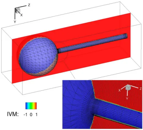
A triangulated surface mesh is used to represent the solid boundary surface for three dimensional problems (see Fig. 1). The vertices and the positive normals (towards the fluid region) of these triangles are stored in a StereoLithography file (STL). Computational cells are divided in three types: solid cells that are inside the solid volume, fluid cells that lie completely in the fluid and cut cells that are intersected by the immersed boundary surface (see Fig. 1).
Figure 1: Top: A three-dimensional Cartesian grid illustrating the three types of cells in the cut-cell approach. The red region (IV M = 1) denotes the fluid cells which lie entirely outside the solid boundary, whereas the blue cells (IV M = −1) denote the solid cells which lie entirely inside the solid boundary. The green cells (IV M = 0) correspond to the cut-cells which are intersected by the internal boundary. Bottom: zoomed-in-view of the part of the immersed boundary region showing the computational cartesian grid.
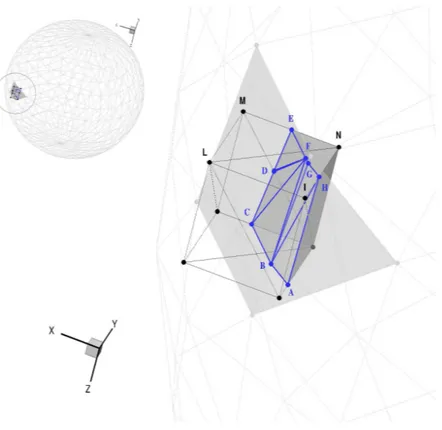
In a first stage, after the production of the cartesian structured computational grid, a marker is assigned to each vertex of the cartesian cell (the grid may not be uniform) that determines whether the vertex is inside or outside the solid. A ray tracing procedure is applied in order to do this [29]. Referring to Fig. 2 a ray is traced from a point A and the number of intersections with the solid triangulated surface is counted. The point A lies inside the solid if the number of intersections is even, outside otherwise. Each computational cell’s face is divided into two triangles whose vertices may be fluid or solid points (see the black bullets in Fig. 2). For
Figure 2: Example of STL boundary surface representation and cut cell. Black line: cut structured cell; Blu line: immersed boundary surface/cut cell intersection; gray line: immersed boundary surface represented by triangulation, gray solid: internal solid part of the immersed boundary.
each cartesian cell face, the intersection points of the triangulated solid boundary surface (A-B-C-D-E-F-G-H-A) with the two triangles of each face are evaluated by a fast triangle/triangle intersection routine [30] and stored in a linking list associated to the computational cell face. The intersection points are ordered to form a polyline (e.g., the connected blue points E-F-G-H in Fig. 2) that divides the face (I-L-M-N) into two polygons respectively in the fluid (E-F-G-H-I-L-M polygon of Fig. 2) and the solid region (E-F-G-H-N polygon). The wet polygon of each face (if exists) is triangularized by a two-dimensional Delaunay triangulation, where the intersection polyline of each face is adopted as a constraint. These boolean operations are performed for all the faces of the original Cartesian cells with at least one internal vertex. The faces’ wet polygons form a polyhedron that is closed by the surface of the immersed solid boundary ∂Γ internal to the computational cartesian cell. In order to characterize this surface, for each intersecting STL triangle, its intersection points with the cartesian face and its internal vertices (if they exist) are stored in a second ordered list associated to the cell (e.g. the three polygons E-F-D, D-F-G-B-C and G-H-A-B in Fig. 2 belonging to different planes). Once the volume of fluid polyhedron is identified by its set of polygons, applying Gauss’s divergence theorem, the wet volume may be calculated for example as:
V = Z V dV = Z ∂Bxˆi · ˆn dS , (12) ˆi and ˆn being the versor of the i − th direction and the normal surface versor, respectively, and
∂B the polyhedron surface. Furthermore, the polyhedron fluid volume centroid coordinates xV i ,
which usually does not coincide with the volumetric center of the original square grid cell, can be calculated as xVi = 1 V Z V xidV = 1 2 V Z ∂B x2idA = 1 2 V Nf X j=1 Z ∂Bj x2i dS, (13) (14) where Nf is the number of polyhedron’s polygonal faces. The centroid coordinates xAi,j of the
j − th face area (“wetted“ or solid) are given by
xAi,j = 1 Aj Z Aj xidA = 1 PNt,j n=1An,j Nt,j X n=1 xi,nAn (15) (16)
Nt,j being the number of triangles and An,j the area of the n − th triangle of the Delaunay
triangulation.
The “wetted“ and solid polyhedron’s areas must be calculated with high precision since in the case of uniform pressure p no source terms related to the pressure gradient are present in the three momentum equations and then the following equation must be satisfied in the i − th coordinate direction: Z ∂B pˆi · ˆ dA = p Z ∂B ˆi · ˆdA = 0 (17) (18) This means that, geometrically, the projection along a fixed direction of the signed wetted
and solid surfaces must be zero (in this work is at least ∼ 10−17m2 ). In classical cut cell
methods, where the internal cutting surface is approximated by a plane, this requirement is naturally fulfilled since the normal versor ˆn and the area of the solid boundary surface S are calculated as: ˆ n = (A + x − A−x |S| , A+ y − A−y |S| , A+ z − A−z |S| ) (19) (20) where |S| =q(A+
x − A−x)2+ (A+y − A−y)2+ (A+z − A−z)2 and A±i being the wetted areas on the
positive/negative faces in the i − th direction.
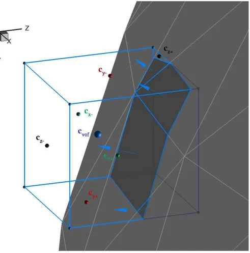
Figure 3 shows the volume of fluid centroid (cvof) where field variables are collocated, the
Figure 3: Example of cut cell geometric characteristics. Blue bullet: cut cell volume of fluid centroid; black bullets: z-normal faces’s centroids; green bullets: x-normal faces’s centroids; red bullets: y-normal faces’s centroid; blue edges with bullets: original cartesian cell; grey surface with blue edges: surface intersection of the immersed body with the cartesian cell; blue arrows: the normals of the immersed surfaces.
Small cell treatment
After calculating all geometric properties of the cut cells, the problem of removing small cut cells has to be taken into account. In fact, the volume of fluid fraction V can be arbitrarily small compared with that of the original cartesian grid cell. These small cell volumes increase the stiffness of the system of equations and restrict the maximum time step that can be used in an explicit time stepping procedure. Special treatment of such cells is necessary for numerical stability and several approaches have been proposed in literature: the application of cell linking [17], cell merging [22], the adoption of a redistribution technique for the cell’s volumes ([20],[19]) and mixed approaches [39]
In this work, the solution of a combined cell-merging/cell-linking approach proposed by Hartmann et al. [39] is adopted. The basic idea is to combine several neighbouring cells together in a newly combined larger cell. To implement this technique, we need first to determine which cells should be merged. A cut cell is considered a slave cell when its volume fraction is less then one half of the original Cartesian cell. Let ns be the mean normal versor of the solid boundary
surface, characterized by Np polygonal surfaces (see Fig. 3): ns = PNp k=1Aknk PNp k=1Ak (21) Ak being the k − th surface area with normal nk. The master cell is chosen in i − th coordinate
direction maximizing the dot product ˆns·(±ˆni), i = 1, 2, 3 , ˆni being the versor of i − th
coordinate direction. When multiple master cells are identified, the greatest is chosen. In the case that the master cell m is a slave cell of another cell m⋆, both s and m become slave cells
of m⋆. The cell volume V
m⋆ and the centroid xVm⋆ of the combined master-slave(s) cluster m⋆
are computed as:
Vm⋆ = Vm+ Ns X k=1 Vsk (22) xVm⋆ = x VmV m+PNk=1s xVskVsk Vm⋆ (23) Ajm⋆ = Ns X k=1 (Ajsk|nki × nj|) (24) xAjm⋆ = x AjmAj m+ PNs k=1(xA j skAj sk|n k i × nj|) Ajm⋆ (25) Ns being the number of slave cells associated to the master cell m, Vsk and x
Vsk the volume
and the volume centroid of the slave cell sk respectively, nki the versor of the i − th direction of
connection between the slave cell sk and the master cell m, Ajsk the slave face area with normal
in the j − th direction. The data are copied to the slave cell(s) sk ∈ S and the master cell
according to xVm ← xVm+S (26) xVsk ← xVm+S, ∀s k ∈ S xAjm ← xAjm⋆ ∂Bm ← ∂Bm+S Vm ← Vm+S Ajm← Ajm⋆.
In this way, all small cells, linked and merged with a suitable master cell m, is treated in the numerical method as passive cells contributing to the balance equations only through fluxes exchange across its surface.
IVM method discretization
In this section, first we describe how performing high order least-squares reconstruction in each cut cell, next we discuss boundary conditions enforcement and advective and diffusive flux
calculation.
Least-Squares interface reconstruction
While fluxes evaluation is straightforward in structured grids, it becomes more difficult at cells cutted by solid boundaries. In the proposed formulation, the least-squares method is adopted to obtain a discretization scheme which is flexible in terms of the local cut cell volume topology and the shape of embedded boundaries and conserves mean value in the control volumes. The cell interface values of the solution variables are found using Taylor series expansion about the cell centroid ci of the volume i:
φIN Tci (x) = φci + ∂φ ∂x ¯ ¯ ¯ ¯ ¯ ci ∆x + ∂φ ∂y ¯ ¯ ¯ ¯ ¯ ci ∆y + ∂φ ∂z ¯ ¯ ¯ ¯ ¯ ci ∆z + ∂ 2φ ∂x2 ¯ ¯ ¯ ¯ ¯ ci ∆x2+∂ 2φ ∂y2 ¯ ¯ ¯ ¯ ¯ ci ∆y2+ (27) +∂ 2φ ∂z2 ¯ ¯ ¯ ¯ ¯ ci ∆z2+ ∂ 2φ ∂x∂y ¯ ¯ ¯ ¯ ¯ ci ∆x∆y + ∂ 2φ ∂y∂z ¯ ¯ ¯ ¯ ¯ ci ∆y∆z + ∂ 2φ ∂x∂z ¯ ¯ ¯ ¯ ¯ ci ∆x∆z
with ∆x = x − xci, ∆y = y − yci, ∆z = z − zci being the distances, along the three cartesian
coordinates, between the reconstruction point and the centroid ci where derivatives in Eqn.
(27) are calculated. Obviously, if a first order reconstruction is required, only the first four terms must be retained in Eqn. (27). The computational stencil of the least squares system, is constructed looking at the neighbouring control volumes ensemble {Sj}i (j = 1, ..., Ni) of
the cut/cartesian cells (the small cut cells are excluded). The control volume ensemble {Sj}i
must include a sufficient number of control volumes for the determination of the derivatives in Eqn. (27). The minimum number of unknowns for the linear and quadratic reconstruction in 3D are 4 and 10 leading to a 2nd and 3rd order accuracy respectively. In practice, in this work, a maximum number of 20 points are used to construct the stencil of the least square method, imposing the conservation of mean in the control volumes and boundary conditions.
The conservation of the mean value within the control volume Vi of the interpolating function
φIN T
ci (x) requires that the following equation must be satisfied:
φi = 1 Vi
Z
Vi
φIN Tci (x) dV. (28)
Substituting the Taylor series, Eqn. (27) in Eqn. (28), collocating the mean value at the volume centroid, gives [40] 0 = ∂φ ∂x ¯ ¯ ¯ ¯ ¯ ci x + ∂φ ∂y ¯ ¯ ¯ ¯ ¯ ci y + ∂φ ∂z ¯ ¯ ¯ ¯ ¯ ci z + ∂ 2φ ∂x2 ¯ ¯ ¯ ¯ ¯ ci x2 2 + ∂2φ ∂y2 ¯ ¯ ¯ ¯ ¯ ci y2 2 + (29) ∂2φ ∂z2 ¯ ¯ ¯ ¯ ¯ ci z2 2 + ∂2φ ∂x∂y ¯ ¯ ¯ ¯ ¯ ci xy + ∂ 2φ ∂y∂z ¯ ¯ ¯ ¯ ¯ ci yz + ∂ 2φ ∂x∂z ¯ ¯ ¯ ¯ ¯ ci xz . with
xmynzp i = 1 Vi Z Vi (x − xci) m (y − yci) n (z − zci) pdV. (30)
that considering the expression of the centroid in Eqn. (13) reduces to calculate moments of the volume Vi respect to ci (using Gauss’ theorem). If a first order reconstruction is adopted,
and the mean value is collocated at the volume of fluid centroid, the conservation of the mean condition is automatically satisfied [18].
Computing the mean value of the reconstruction φIN T
ci (x) in a volume Vj of the ensemble
{Sj}i, that forms the compact stencil of the least square method, implies that:
φj = 1 Vj Z Vj φIN Tci (x) dV = φi+ ∂φ ∂x ¯ ¯ ¯ ¯ ¯ ci à 1 Vj Z Vj (x − xci) dV ! + + ∂φ ∂y ¯ ¯ ¯ ¯ ¯ ci à 1 Vj Z Vj (y − yci) dV ! +∂φ ∂z ¯ ¯ ¯ ¯ ¯ ci à 1 Vj Z Vj (z − zci) dV ! + ∂ 2φ ∂x2 ¯ ¯ ¯ ¯ ¯ ci à 1 Vj Z Vj (x − xci) 2dV ! +∂ 2φ ∂y2 ¯ ¯ ¯ ¯ ¯ ci à 1 Vj Z Vj (y − yci) 2dV ! (31) + ∂ 2φ ∂z2 ¯ ¯ ¯ ¯ ¯ ci à 1 Vj Z Vj (z − zci) 2dV ! + ∂ 2φ ∂x∂y ¯ ¯ ¯ ¯ ¯ ci à 1 Vj Z Vj (x − xci)(y − yci) dV ! + ∂ 2φ ∂y∂z ¯ ¯ ¯ ¯ ¯ ci à 1 Vj Z Vj (y − yci)(z − zci) dV ! + ∂ 2φ ∂x∂z ¯ ¯ ¯ ¯ ¯ ci à 1 Vj Z Vj (x − xci)(z − zci) dV !
Following the work of Gooch [40] in order to avoid the calculation of moments of each control volume Vj with respect to ci, in Eqn. (31) x − xci,y − yci,z − zci are replaced with
(x − xcj) + (xcj− xci), (y − ycj) + (ycj− yci), (z − zcj) + (zcj − zci) respectively: φj = φi+∂φ ∂x ¯ ¯ ¯ ¯ ¯ ci ˆ x + ∂φ ∂y ¯ ¯ ¯ ¯ ¯ ci ˆ y + ∂φ ∂z ¯ ¯ ¯ ¯ ¯ ci ˆ z + ∂ 2φ ∂x2 ¯ ¯ ¯ ¯ ¯ ci ˆ x2+ ∂ 2φ ∂y2 ¯ ¯ ¯ ¯ ¯ ci ˆ y2 (32) +∂ 2φ ∂z2 ¯ ¯ ¯ ¯ ¯ ci ˆ z2+ ∂ 2φ ∂x∂y ¯ ¯ ¯ ¯ ¯ ci ˆ xy + ∂ 2φ ∂y∂z ¯ ¯ ¯ ¯ ¯ ci ˆ yz + ∂ 2φ ∂x∂z ¯ ¯ ¯ ¯ ¯ ci ˆ xz with \ xnymzp = 1 Vj Z Vj ³ (x − xcj) + (xcj − xci) ´n³ ((y − ycj) + (ycj − yci) ´m³ ((z − zcj) + (zcj − zci) ´p dV (33) = p X r=0 ( p! r!(p − r)!(zcj − zci) r m X l=0 ( m! l!(m − l)!(ycj − yci) l m X l=0 h n! k!(n − k)!(xcj − xci) kxn−kym−lzp−ri ))
∆φ = S dφ (34) where ∆φ = 0 φ1− φci φ2− φci ... ... φNi− φci (35) S = xi yi zi x2i y2i z2i xyi yzi xzi b x1 by1 bz1 xb21 yb21 zb21 cxy1 cyz1 cxz1 b x2 by2 bz2 xb22 yb22 zb22 cxy2 cyz2 cxz2 ... ... b xNi byNi bzNi xb 2 Ni yb 2 Ni zb 2 Ni xycNi cyzNi cxzNi (36) dφ = h ∂φ∂x ∂φ∂y ∂φ∂z ∂∂x2φ2 ∂2φ ∂y2 ∂2φ ∂z2 ∂2φ ∂x∂y ∂2φ ∂y∂z ∂2φ ∂z∂x i (37) The system of equation (34) becomes:
(STS)−1ST∆φ = C ∆φ = dφ (38)
where the C matrix has dimension (Ni+ 1) x (Ni+ 1), it contains only geometric constants, and
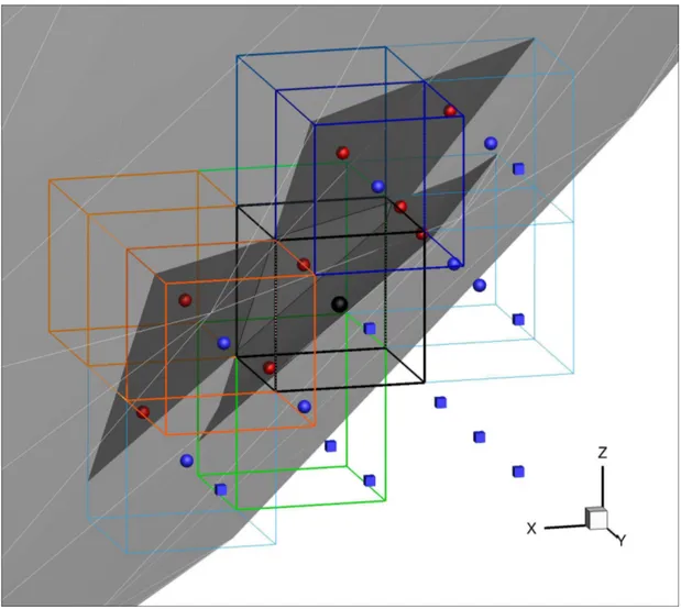
it may be computed and stored in a preprocessing stage. Figure 4 shows, for a scalar centroid, the interpolation stencil used for the determination of the least square system (34).
Application of boundary conditions
Boundary conditions are imposed in Eqn. (34) by prescribing the values of a variable or its derivatives on specific auxiliary points of the boundary surface. Each point is created for the cut cell, by finding the intersection point xib of the line passing from the volume of fluid centroid
having the direction of the mean normal to the solid surface ∂B. Given the mean normal of the boundary cutting surfaces Eqn. (21), if one of the normals of the triangulated boundary surface (e.g., the edge of a cube intersecting a cartesian grid), forms an angle greater then a fixed value (30◦ in this work), other boundary points are added as boundary constraints (surface
centroids). For example, the velocities no-slip condition for a non-moving body (a Dirichlet boundary condition) is imposed at these auxiliary points xib by means of φ
IN T(x
ib) = φ(xib) =
0, ib = 1..Nb (Nb is the number of boundary points in the interpolation cloud) in the vector ∆φ
Figure 4: Example of points cloud used for the interpolation of scalar variables. White line: stl surface trian-gulation; black line: original cartesian volume of the cut cell and its boundary cutting surface; red bullets: surface boundary points; blue bullets: the serrounding volume of fluid centroids; blue cube: centroid of the second layer cells; cartesian edges: different colour shades indicate cut cells forming master-slave pair (green and orange).
φIN Tci (xib) = φci+ ∂φ ∂x ¯ ¯ ¯ ¯ ¯ ci ∆xib + ∂φ ∂y ¯ ¯ ¯ ¯ ¯ ci ∆yib+ ∂φ ∂z ¯ ¯ ¯ ¯ ¯ ci ∆zib + ∂2φ ∂x2 ¯ ¯ ¯ ¯ ¯ ci ∆xib 2+ ∂2φ ∂y2 ¯ ¯ ¯ ¯ ¯ ci ∆yib 2+ (39) ∂2φ ∂z2 ¯ ¯ ¯ ¯ ¯ ci ∆zib 2+ ∂2φ ∂x∂y ¯ ¯ ¯ ¯ ¯ ci ∆xib∆yib+ ∂2φ ∂y∂z ¯ ¯ ¯ ¯ ¯ ci ∆yib∆zib+ ∂2φ ∂x∂z ¯ ¯ ¯ ¯ ¯ ci ∆xib∆zib,
∆φ = 0 φ(x1b) − φci φ(x2b) − φci ... φ(xNb) − φci φNb+1− φci ... ... φNi− φci (40) S = xi yi zi x2i y2i z2i xyi yzi xzi ∆x1b ∆y1b ∆z1b ∆x 2 1b ∆y 2 1b ∆z 2 1b ∆x1b∆y1b ∆y1b∆z1b ∆x1b∆z1b ∆x2b ∆y2b ∆z2b ∆x 2 2b ∆y 2 2b ∆z 2 2b ∆x2b∆y2b ∆y2b∆z2b ∆x2b∆z2b ... ∆xNb ∆yNb ∆zNb ∆x 2 Nb ∆y 2 Nb ∆z 2 Nb ∆xNb∆yNb ∆yNb∆zNb ∆xNb∆zNb b x1 yb1 bz1 xb21 yb21 zb21 xyc1 cyz1 cxz1 b x2 yb2 bz2 xb22 yb22 zb22 xyc2 cyz2 cxz2 ... ... b xNi ybNi bzNi xb 2 Ni yb 2 Ni zb 2 Ni xycNi yzcNi cxzNi (41) The red and blue colors of the matrix coefficients in Eqn. (40) and (41) refers to the points showed in Fig. 4 representing boundary points and volume of fluid centroids respectively.
After calculating the gradient of Eqn. 27 at a boundary point xib, multiplying it by the
component of the local normal direction nib, it is possible to evaluate the normal derivative and
impose a Neumann boundary condition ∂φ(xib)
∂n = gn(xib): ∇φIN Tci (xib) · nib = ( ∂φ ∂x ¯ ¯ ¯ ¯ ¯ ci + ∂ 2φ ∂x2 ¯ ¯ ¯ ¯ ¯ ci ∆xib+ ∂2φ ∂x∂y ¯ ¯ ¯ ¯ ¯ ci ∆yib+ ∂2φ ∂x∂z ¯ ¯ ¯ ¯ ¯ ci ∆xib) nibx+ (42) +(∂φ ∂y ¯ ¯ ¯ ¯ ¯ ci + ∂ 2φ ∂y2 ¯ ¯ ¯ ¯ ¯ ci ∆yib+ ∂2φ ∂x∂y ¯ ¯ ¯ ¯ ¯ ci ∆xib+ ∂2φ ∂y∂z ¯ ¯ ¯ ¯ ¯ ci ∆zib) niby+ +(∂φ ∂z ¯ ¯ ¯ ¯ ¯ ci +∂ 2φ ∂z2 ¯ ¯ ¯ ¯ ¯ ci ∆zib+ ∂2φ ∂y∂z ¯ ¯ ¯ ¯ ¯ ci ∆yib+ ∂2φ ∂x∂z ¯ ¯ ¯ ¯ ¯ ci ∆xib) nibz = gn(xib)
S = xi yi zi x2i y2i z2i xyi yzi xzi
nx1b ny1b nz1b ∆x1bnx ∆y1bny ∆z1bnz ∆y1bnx+ ∆x1bny ∆y1bny+ ∆z1bny ∆x1bnz+ ∆z1bnx
nx2b ny2b nz2b ∆x2bnx ∆y2bny ∆z2bnz ∆y2bnx+ ∆x2bny ∆y2bny+ ∆z2bny ∆x2bnz+ ∆z2bnx
... ... ...
nxNb nyNb nzNb ∆xNbnx ∆yNbny ∆zNbnz ∆yNbnx+ ∆xNbny ∆yNbny+ ∆zNbny ∆xNbnz+ ∆zNbnx
b x1 by1 zb1 cx21 cy21 zb21 cxy1 cyz1 cxz1 bx2 by2 zb2 cx22 cy22 zb22 cxy2 cyz2 cxz2 ... ... ... ... ... ... b xNi byNi zbNi cx 2 Ni cy 2 Ni zb 2 Ni cxyNi yzcNi cxzNi (43) while the vector ∆φ is:
∆φ = 0 g(x1b) g(x2b) ... g(xNb) φNb+1− φci ... ... φNi− φci (44)
In this work, no slip boundary conditions for all the three velocity components and Neumann boundary conditions ∂φ(xib)
∂n = 0) for density, energy and species mass fraction, are applied at
boundary points (determined as described in the initial section of this paragraph) , while Neumann boundary conditions are enforced at Gauss boundary integration points for pressure.
Fluxes calculation
Integrating Eqns. (1-4) over the volume Vi of the cut cell and using the divergence theorem:
∂Q ∂t = 1 Vi Z ∂Bi F · ndA + S (45) (46) where Q = [ρ, ρu, ρU, ρYi]T, is the vector of conserved variables, S = [0, 0, 0, ρ ˙ω]T, F = Finv+Fv
being the flux vector containing an inviscid part Finv and a viscous part Fv, and n the outward
unit normal vector to the cut cell surface dA.
The inviscid surface integral in Eqn. (45) is approximated as: 1 Vi Z ∂Bi Finv · ndA = 1 Vi Nf X j=1 Z ∂Aj Finvnj (Q L, QR) dA j (47) (48) Here, Finv nj (Q
L, QR) represents the numerical convective flux in the direction normal to the
solution UL/R on both sides of A
j. The superscripts ”R” and ”L” refer to the spatial limit
respectively on the outside and inside of the cut cell Vi with respect to its face Aj. In particular
QL represents the solution calculated on the face A
j using the interpolation function φIN Ti in
Vi, while QR represents the reconstructed solution calculated on Aj using the interpolation
function φIN T
j in the neighbouring cell Vj (Vj cell may be a cut cell or a second layer cell).
Since the flux Finv nj (Q
L, QR) varies along the face A
j (quadratically in this work), it must
be evaluated at each Gauss point xg (or at the face centroid when linear reconstruction is
adopted). The flux is formulated using a modified version of the advection upstream splitting method (AUSM) [41]. In this method, the inviscid flux is split into a convective component
and a pressure term involving the Mach number Mg = vg/ag, such that the numerical inviscid
flux Fj(xg), can be computed as
Fj(xgj) = 1 2 © Mjm[(fj)L+ (fj)R] + |Mjm|[(fj)L− (fj)R] ª + pm (49) where Mjm = 0.5((fj)L+ (fj)R) (50) and fj = ρc ρcu c(ρU + p) cρYn .
ρ, c, u, U, Yi being density, sound velocity, velocity vector, total energy, species mass fraction
respectively. The pressure term pm is computed such that
pm = ½ (pm)L · 1 2 + χ ¡ Mjm¢L ¸ + (pm)R · 1 2 − χ ¡ Mjm¢R ¸¾ 0 um 0 0 . (51)
where a dissipative splitting at χ = 0.5 is used to dump spurious oscillations.
With the details of the gradient expression in mind (eq.42), viscous flux Fv in Eqn. 45
are now derived. First, it is calculated the gradient at the centroid xAj of the face A
j (the
gradient varies linearly inside each cut cell) from the reconstruction functions φIN T
i in Vi and
φIN T
j in the neighbouring cell Vj. The surface gradient is computed as a distance weighted
convex combination of cell center gradients:
∇φ(xf) = wi∇φIN Ti (xf) + wj∇φIN Tj (xf) (52) with ( wi = |xci−xf| |xci−xf|+|xcj−xf| wj = 1 − wi (53)
Due to the staggering, for each type of cut cell Vi (velocity or scalars) and for each of the
6 possible wetted polyhedron’ faces, the index of the corresponding neighbouring cell Vj is
required to reconstruct the left and right solutions. All the required indexes are stored in a pre-computed list (see Fig. 5), readily available at runtime calculation.
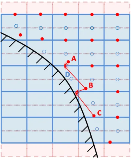
Figure 5 shows the neighbouring centroids (red bullets) of the Uz interpolation function
used to calculate the left and right states on the positive (A,B centroids) and negative (B,C centroids) faces with normal versor parallel to the z direction of a ρ cut cell (the centroid D, indicated with a blue open circle).
Figure 5: Interpolation functions of ρUz used to calculate left and right states on density cut cell. Blue open
circles: density centroids; red circles: ρUz centroids; red dot-line grid: original cartesian ρUz grid;
blue line grid: original cartesian ρ grid; black line: boundary surface.
To compute wall shear stress on the boundary surfaces of no-slip walls of a cut cell Vi,
the components of the stress tensor τ(xbi) (i = 1..Np) must be calculated at the cut cell’s
boundary face centroids. In the general case of a boundary surface constituted by Np polygons
with different normals (this is the case of high curvature boundary surfaces immersed in coarse cartesian grid), the expression of the viscous flux integral related to the boundary surface in Eqns. (45) is approximated as
1 Vi Z ∂Bw Fv· ndA = 1 Vi Np X k=1 τ (xbk) · nkdAk (54) (55)
with ∂Bw the wall boundary surface of the cut cell Vi, nk the versor of k − th boundary
polygonal surface, τ the stress tensor calculated specifing velocity gradients ∇uIN T
x (x, y, z),
∇uIN T
y (x, y, z), ∇uIN Tz (x, y, z) at the k − th boundary surface centroids xbk.
In order to couple the finite volume method of the Immersed Volume method and the finite difference general code, the convective or diffusive term F in the transport equation for a second layer cell is calculated as:
Fi =
fIV M
i,p ci,p+ fi,nIV Mci,n+ fi,pf d(1 − ci,p) + fi,nf d(1 − ci,n)
V ol2l
(56) where V ol2l is the volume of the second layer cell, fi,pIV M is the flux, on the positive face p (n,
stands for the negative one) with normal i, calculated by the finite volume solver of the IVM method, ff d
i,p that calculated by the general finite difference code and the coefficient ci,p(n) is 1
if the positive (negative) face is in contact with a cut cell, 0 otherwise.
Numerical results and validation
The accuracy and robustness of the Immersed Volume Method is validated by computing two three-dimensional test cases. The solver has been fully parallelized using the Message Passing Interface (MPI) libraries such that parallel computations on shared and distributed memory systems are possible.
Flow past a cube at
Re = 215
The flow past a cube is an appropriate validation test case, because of the presence of sharp edges boundaries, cut cells with internal volume and faces centroid. The Reynolds number
based on the freestream velocity is defined as Reedge = ρuLµ∞ = 215, with L being the edge
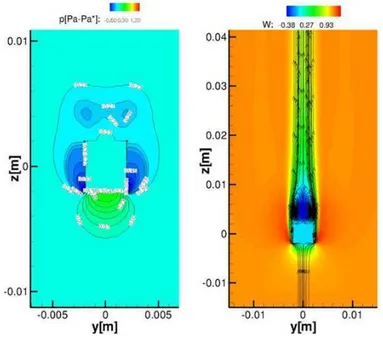
lenght of the cube. For the three-dimensional simulation of a uniform flow past a cube, a computational domain Ω: [-2.5L, 2.5L]x[-2.5L, 2.5L]x[-2.5L, 7.5L] is used, with the midpoint of the cube located at the system origyn. The cartesian domain contains approximately 3.0 million of cells. The grid is refined near the cube edges in all directions. Computations for this Reynolds number found a symmetric and steady flow as shown in Fig. 6 where the instantaneous pressure and axial velocity contour around the cube are reported. The recirculating lenght is 2.73 ([42]), while the drug coefficient is 0.864 (0.866 from the classical fit Drug coefficient curve[42]).
Is clearly visible the expansion that occurs near the edge of the cube and the consequent speed increase (see Fig. 6 ). Despite the presence of cube’s edges, and so of strong gradients of velocities, the streamtraces are very regular, (see Fig. 6 ) this confirm the stability of the new proposed method.
Figure 6: Flow past a cube: left) color map of pressure at the plane x-z, and y=0; right) snapshot of the axial velocity at the plane x-z, and y=0.
Flow past a sphere at
Re = 51500
In this section the LES of the Bakic experiment [46] of the flow past a sphere with sting at Re = 51500 is presented. Several simulations of the flow past a sphere in the sub-critical regime have been carried out, contributing to a better understanding of fluid and vortex-shedding dynamics. Tomboulides et al. [47] performed time-accurate direct numerical simulation up to Re = 1000. Costantinescu et al. carried DES for studying the flow behind a sphere for the sub-critical
and supercritical regimes at Reynolds numbers in the range of 104 − 106 [48]. More recently
Rodriguez et al. [49] performed DNS of the flow over a sphere in the subcritical regime at Re = 3700, determining the separation point and vortex shedding characteristics frequencies. The Reynolds number based on the freestream velocity is defined as ReD = ρ∞µu∞∞D = 51500, with
D being the sphere diameter (0.0614 m). For the three-dimensional simulation of the flow past a sphere, a cartesian computational domain Ω: [−1.7D, 5D]x[−4.88D, 4.88D]x[−4.88D, 4.88D] is used with [280]x[140]x[140] points in the z (streamwise), x and y directions respectively. The midpoint of the sphere is located at the system origyn. The grid is locally refined near the surface of the sphere, along the stick (that has a diamater d of 0.13D) and near the separation
regions. The free stream air velocity U∞ is 12.6 m/s and the corresponding Mach number
M a∞ = U∞/c∞ = 0.037. The inlet turbulence level is 0.56% and these turbulent inflow
boundary conditions are artificial prescribed by means of the Klein procedure [50].
Premixed
CH
4/Air past a cube at Re = 3200
The flow past a cube with combustion is chosen as an appropriate validation test case, because of its sharp edge boundaries, cut cells with internal volume and faces’ centroids and sharp density
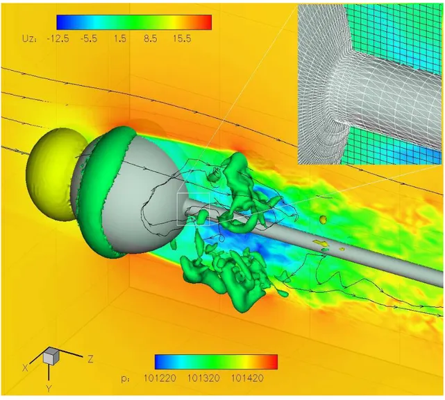
Figure 7: Instantaneous axial velocity; pressure isosurfaces at 101317 Pa and 101409 Pa. Zoomed in view: STL of the solid surface (white lines) and simulation grid (black lines).
and velocities gradients. The Reynolds number based on bulk quantities at the duct section
(assuming its half width as reference length) crossing the cube leading edge is ReLED = 3200
and the maximum Mach number is ∼ 0.05. For the three-dimensional simulation of a uniform flow past a cube, a computational domain Ω:[−2L, 3.5L]x[−2L, 2L]x[−2L, 2L] is used, L being the cube size.
A reduced kinetic mechanisms for the CH4 with 5 chemical reacting species and 3 reactions
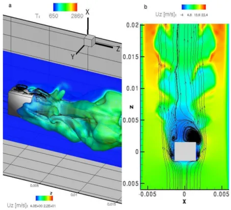
is adopted. The premixed stoichiometric mixture is preheated up to 650K since with an inlet temperature of 300K the flame is stretched by high velocity gradients. The cartesian not uni-form domain has 120x80x80 grid points in the axial and spanwise directions. It is clearly visible the separation region that occurs near the lower edge of the cube and the consequent formation of a lateral first recirculation region at the side walls immediately after the separations. The flame is attached in the second recirculation region downstream of the cube bluff-body and because the first lateral vortex is able to go up stream up to the leading edge of the cube (see Fig. 8).
Figure 8: Premixed flame past a cube: a) Temperature isosurface (1500K) coloured by axial velocity Uz and
Temperature slice; b) x-z plane of instantaneous Uz with streamlines.
0.1
Conclusions
A cut-cell based Cartesian grid method for three-dimensional compressible flows and not-uniform staggered grid is presented. The small-cell problem inherent in Cartesian cut-cell methods is solved using a cell-merging/cell-linking technique. The effective treatment of the small cells enabled the use of rather large CFL numbers in simulations. The accuracy of the viscous fluxes is second order. Along with this extension, the solver is currently being extended for combustion problems and heat transfer between the solid and the fluid flow.
Bibliography
[1] K. Akselvoll, P. Moin, Large-eddy simulation of turbulent confined coannular jets, J. Fluid Mech. 315 (1996) 387.
[2] C.D. Pierce, Progress-variable approach for large eddy simulation of turbulent combustion, Ph.D. thesis, Stanford University, 2001.
[3] S. Nagarajan, S.K. Lele, J.H. Ferziger, A robust high-order compact method for large eddy simulation, Journal of Computational Physics 191, (2003) 563-582.
[4] F.K. Chow, P. Moin, A further study of numerical errors in Large Eddy Simulations, Journal of Computational Physics 184, (2003) 366-380.
[5] S. Ghosal, An analysis of numerical errors in Large Eddy Simulation of turbulence, Journal of Computational Physics 125, (1996) 187-206.
[6] F.E.Ham,F.S. Lien, A.B. Strong, A fully conservative second-order finite difference scheme for incompressible flow on non unifrom grids, Journal of Computational Physics 191, (2002) 117-133.
[7] D.A. Kopriva, A staggered-grid multidomain spectral method for the compressible NavierâStokes equations, Journal of Computational Physics 143 (1998) 125.
[8] G.S. Djambazov, C.H. Lai, K.A. Pericleous, Staggered-mesh computation for aerodynamic sound, AIAA J. 38 (2000) 16.
[9] E.A. Fadlun, R. Verzicco, P. Orlandi, J. Mohd-Yusof, Combined immersed-boundary finite-difference methods for three-dimensional complex flow simulations, Journal of Computa-tional Physics 161 (2000) 35-60.
[10] J. Mohd-Yusof, Combined immersed boundary/B-splines methods for simulations of flows in complex geometries, in: Center for Turbulence Research Briefs, NASA Ames/Stanford University, 1997.
[11] F. Muldoon, S. Acharya, A divergence free interpolation scheme for the immersed boundary method, Int. J. Numer. Method Fluid 56 (2008) 1845-1884.
[12] S. Kang, G. Iaccarino, P. Moin, Accurate immersed boundary reconstractions for viscous flow simulations, AIAA J. 47 (7) (2009) 1750-1760.
[13] D. Clarke, M. Salas, H. Hassan, Euler calculations for multi-elements airfoils using Carte-sian grids, AIAA J. 24 (3) (1986) 353-358.
[14] M.J. Berger, R.J. Leveque, Stable boundary condition for cartesian grid calculations, Com-puter System in Engineering 1 (1990) 305-311.
[15] H. Johansen, P. Colella, A cartesian grid embedded boundary method for Poisson’s equa-tion on irregular domains, Journal of Computaequa-tional Physics 147 (1998) 60-85.
[16] M.H. Chung, Cartesian cut cell approach for simulating incompressible flows with rigid bodies of arbitrary shape, Comput. Fluid 35 (2006) 607-623.
[17] M.P. Kirkpatrick, S.W. Armfield, J.H. Kent, A representaion of curved boundaries for the solution of the Navier-Stpkes equations on a staggered three-dimensional Cartesian grid, Journal of Computational Physics 184 (2003) 1-36.
[18] D. Heartmann, M. Meinke, W. Schroderm, A strictly conservative Cartesian cut-cell method for compressible viscous flows on adaptive grids, Comp. Methods Appl. Mech. Engrg. 200 (2011) 1038-1052.
[19] M. Mayer, A. Devesa, X.Y. Hu, N.A. Adams, A conservative immersed interface method for Large-Eddy Simulation of incompressible flows, Journal of Computational Physics 229 (2010) 6300-6317.
[20] X.Y. Hu, B.C. Khoo, N.A. Adams, F.L. Huang, A conservative interface method for com-pressible flows, Journal of Computational Physics 219 (2006) 553-578.
[21] Y. Cheny, O. Botella, The LS-STAG method: A new immersed/level-set method for the computation of incompressible viscous flows in complex moving geometries with good conservation properties, Journal of Computational Physics 229 (2010) 1043-1076.
[22] J.H. Sao, R. Mittal, A sharp-interface immersed boundary method with improved mass conservation and reduced spuroius pressure oscillations, Journal of Computational Physics 230 (2011) 7347-7363.
[23] F.H. Harlow, J.E. Welch, Numerical calculation of time-dependent viscous incompressible flow of fluid with free surfaces, Phys. Fluid 8 (1965) 2181-2189.
[24] R.W.C.P. Verstappen, A.E.P. Veldman, Symmetry-preserving discretization of turbulent flow, Journal of Computational Physics 187 (2003) 343-368.
[25] C. Günther, D. Hartmann, M. Meinke, W. Schroder, A level-set based cut-cell method for flows with complex moving boundaies,V European Conference on Computational Fluid Dynamic, Lisbon, Portugal,14-17 June 2010.
[26] H. Ji, F.S. Lien, E. Yee, NUerical simulation of detonation using an adaptive Cartesian method combined with a cell-merging technique, Computers and Fluids, 39,6, (2010), 1041-1057.
[27] Yang G., Causon D.M., Ingram D.M., Saunders R., Batten P., A Cartesian cut cell method for compressible flows â part B: moving body problems. Aeronautical Journal 101 (1997) 57-65.
[28] Chiang Y., Van Leer B., Powell K.G., Simulation of unsteady inviscid flow on an adaptively refined Cartesian grid, AIAA Paper (1992) 92-0443-CP.
[29] M.J. Aftosmis, M.J. Berger, J.E. Melton, Robust and efficient cartesian mesh generation for component based geometry, Tech. Report AIAA-97-0196, US Air Force Wright Laboratory, (1997).
[30] T. Moller, A Fast Triangle-Triangle Intersection Test, Journal of Graphics Tools, 2(2), 1997.
[31] T. Poinsot, D. Vaynante, Theoretical and numerical combustion, 2012.
[32] E. Giacomazzi, V. Battaglia and C. Bruno, The Coupling of Turbulence and Chemistry in a Premixed Bluff-Body Flame as Studied by LES, Combustion and Flame, 138 (2004) 320-335.
[33] R.B. Bird, W.E. Stewart, E.N. Lightfoot, Transport Phenomena, Wiley International Edi-tion, (2002).
[34] C.R. Wilke, J. Chem. Phys., 18, (1950), 517-9.
[35] R.J. Kee, G. Dixon-Lewis, J. Warnatz, M.E. Coltrin, Miller JA, Moffat HK, The CHEMKIN Collection III: Transport, San Diego, Reaction Design, (1998).
[36] S. Mathur, P.K. Tondon, S.C.Saxena, Molecular Physics, 12:569, (1967).
[37] E. Giacomazzi, F.R. Picchia, N.M. Arcidiacono, A Review on Chemical Diffusion, Criti-cism and Limits of Simplified Methods for Diffusion Coefficients Calculation, Combustion Theory and Modelling, (2008).
[38] C.W. Shu, S. Osher, Efficient implementation of essentially non-oscillatory shock-capturing schemes, Journal of Computational Physics, 77, 439-471 (1988).
[39] D. Hartmann, M. Meinke, W. Schr¨der, An adaptive multilevel multigrid formulation for Cartesian hierarchical grid methods, Comput. Fluids 37 (2008).
[40] C. O. Gooch, M.Alten, A High order accurate unstructured mesh Finite Volume scheme for the advection diffusion equation, Journal of Computational Physics, 181, 729-752 (2002). [41] M.S. Liou, C.J. Steffen Jr., A new flux splitting scheme, Journal of Computational Physics
107 (1993) 23-39.
[42] A.K. Saha, Three dimensional numerical simulations of the transition of flow past a cube, Journal of Computational Physics 16, 2004.
[43] J.C. Mandal, S.P. Rao, High resolution finite volume computations on unstructured grids using solution dependent weighted least square gradients, Comput. Fluids, 2010.
[44] J.C. Mandal, J. Subramanian, On the link between weighted least-squares and limiters used in higher-order reconstructions for finite volume computations of hyperbolic equations, Appl Numer Math, 2008;58:705-25.
[45] D. Levin, The approximation power of moving least-squares, Math. Comput. 224 (1998), 1517-1531.
[46] V. Bakic, M. Schmid, B. Stankovic, Experimental Investigaion of Turbulent Structures of Flow Around a Sphere, Thermal Scinces, 10 (2006), 97-112.
[47] A. Tomboulides, S. Orszag, Numerical Investigation of Transitional and Weak Turbulent Flow past a Sphere, Journal of Fluid Mechanics, 416, (2000), 45-73.
[48] G. Costantinescu, K. Squires, Numerical Investigations of flow over a sphere in the sub-critical and supersub-critical regimes, Phys. Fluids, 16, (2004), 1449-1466.
[49] I. Rodriguez, R. Borell, O. Lehmkuhl, C.D. Perez Segarra, A. Oliva, Direct Numerical Simulation of the flow over a sphere at Re = 3700, Journal of Fluid Mechanics, 679, (2011), 263-287.
[50] M. Klein, A. Sadiki, J. Janicka, A digital filter based generation of inflow data for spatially developing direct numerical or large eddy simulations, Journal of Computational Physics 186, (2003), 652-665.