215
Appendix A
Some consideration about thermodynamic indicators
for renewable energies
A.1. Definition of the First-Law efficiency for renewable energies
With respect to renewable energy systems some appreciations must be made in order to clarify the definition of the first-law efficiency. For wind and hydro power plants, the traditional first-law efficiency indicator use to be the performance efficiency of the machine, while for photovoltaic power systems first-law efficiency is applied to the panel efficiency. However, this indicator does not take into considerations the fluctuations of the wind velocity and of the water stream or the solar intensity varying in time. Because, as will be shown further, this efficiency depends also on the wind speed distribution for wind power plants, on the variance of the total water flow for hydro power plants and on the solar intensity for photovoltaic power systems.
Therefore an attempt to define the first-law efficiency indicators for solar, wind a hydro power plants as a relation of the energy produced and the energy producible is given. This definition may contribute towards a better insight of what is needed for an accurate
Appendix A. Some consideration about thermodynamic indicators for renewable energies
216
description of technical indicators. This indicator included considerations about fluid dynamics and wind speed power density function. In fluid dynamics studies, the available fluid power becomes as shown in eq. A.1.
3 avail A 2 1 ) ( P υ = ρ υ (A.1)
Where ρ is the fluid density, A is the cross section area and ν is the fluid velocity.
The eq. A.1, characterizes the dynamic power available in a fluid, being able to describe the availability power of a fluid incident in a turbine with a rotor swept area A for given fluid density and speed. This can be applied for water and wind as fluids and, therefore, to calculate availability power for wind and hydro turbines.
Consequently, wind power is related to the cube of the wind speed, but considering that wind velocity varies continuously in time and site. Power wind depends, as well, on the wind speed probability density function.
In order to calculate the wind speed probability density function, two methodologies can be applied; i) the collection of wind speed data for a potential site. These are often based on finite measurements over a fixed period of time in one location. A long-term multipoint array of wind statistics is desirable to better characterize the site and specific locations for turbine sitting. ii) the Weibull density function. This function can model closely wind speed variations, eq. A.2.
2 c 2 e c 2 ) ( f υ υ = υ 0 < ν < ∞ (A.2)
Where c is a scalar parameter.
The general pattern of wind speed described by the Weibull density function distribution gives us the probability of each wind speed, see Fig. A.1.
217
probability density function from the Weibull graph is obtained the distribution of wind energy at different wind speeds, the power density function that varies in proportion to the cube of the wind speed and the air density.
For an ideal wind turbine, the wind energy available in the wind can be completely extracted so that the turbine rotor starts to function at cut-in speed Vcut-in and power
generated increases as wind speed increases until it reaches the rated wind speed VR. At
wind speeds between the rated wind speed and the cut-off wind speed Vcut-off, a constant
rated power is generated corresponding to substitute in eq. A.1, ν per νR. At wind
velocities exceeding cut-off wind speed, the turbine is completely shut down. As a result the wind energy generated by an ideal wind turbine operated at an increasing relation of power between cut-in and rated wind speed and a constant tare power PR between rated
and cut-off wind speed can be given by:
υ υ + υ υ υ =
∫
∫
− − R R V in Vcut off Vcut v R ideal T P( )f( )d P f( )d E (A.3)Appendix A. Some consideration about thermodynamic indicators for renewable energies
218
Where T is the time period, P(ν) is the availability power function for a wind turbine, eq. A.1 and f(ν) is the Weibull density function given by eq. A.2
For a real wind turbine, the power in the wind is converted into the mechanical-rotational energy of a wind turbine rotor, which would reduce the speed of the air mass. The wind energy available cannot be extracted completely by any real wind turbine, so the availability power function for a wind turbine, eq. A.1 cannot be applied. Instead of, for wind turbines that operate at constant power PR with maximum efficiency between rated
and cut-out speed and at increasing power between cut-in and rated speed, the actual wind power output from the wind turbine PT is determinated by the turbine performance
curve, which is well describe by the following expression A.4: The power function for a wind turbine can be describe where the wind turbine energy potential per second, varies in proportion to the cube of the wind speed, for a minimum and a maximum wind speed, see Fig. A.2.
υ ≥ υ υ < υ ≤ υ υ < υ ≤ υ + υ + υ + υ υ < υ = υ − − − − off cut off cut R R R 1 in cut R 4 3 2 2 3 1 in cut T , 0 , P , P ) a a a a ( , 0 ) ( P (A.4)
Where a1, a2, a3, and a4 are regression constants of the turbine performance curve.
Figure A.2: Typical wind turbine power curve
PT PT
219
T(ν) multiplied by the probability of the wind speed
experienced f(ν) and integrated over all possible wind speed.
( ) ( )
∫
− − υ υ υ = out Vcut in Vcut T A T P f d E (A.5)Therefore, since the wind energy available in the wind cannot be completely extracted by any wind turbine, the wind turbine efficiency defined as the ratio of the actual wind energy output from a wind turbine to the wind energy generated by an ideal wind turbine, is meaningful for evaluating turbine performance an is expressed as the ration of eq.A.6.
ideal A E E = η (A.6)
From eq. A.6 can be seen that the wind turbine efficiency is not only a function of wind turbine performance, but also a function of wind speed distribution. Analogous argumentation is true for hydropower systems, where the hydro turbine efficiency depends also on the water flow distribution function1.
For photovoltaic energy systems the function of the solar energy reaching the panel can not be modeled so easy as for wind speed. Since the solar intensity depends on the latitude, the year’s day, the day time, the panel position and on the azimuthal angle. Therefore, the definition of the solar intensity function requires of an accurate study of the determined site, where the photovoltaic panel should be placed. The first-law efficiency will be also defined as the ratio between the energy produced and the integral of the energy producible, which include considerations about the solar radiation reaching the panel, better that the pane efficiency of radiation’s transformity.
Appendix A. Some consideration about thermodynamic indicators for renewable energies
220
A.2. Definition of the Second-Law efficiency for renewable energies
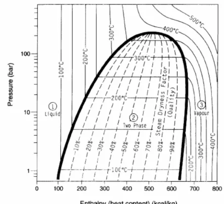
Furthermore, considerations about the second-law efficiency indicator for renewable energy systems offer specific definition for geothermal power stations to be taken into account.The geothermal systems have resources of hydrothermal reservoirs that can produce water either in compressed liquid water phase or as superheat water vapor, these fields are traditionally classified as: Water dominant or Vapor dominant, the latter having a higher energy content per unit fluid mass. The production of steam and water from a geothermal reservoir can be illustrated on a pressured-enthalpy diagram for pure water, as shown in Fig. A.3. The water dominant plant is located in zone 1, while the vapor dominant is located in zone 3.
Figure A.3: pressure versus enthalpy diagram for pure water and steam, with
thermodynamic fluid reservoir conditions, (1) liquid water, (2) two-phase liquid steam and water, (3) superheat steam.2
221 components constituting the vapor.
The second law efficiency for these systems can be described as below:
) S T h ( m W 0 vapor vapor . out II − = η (A.7)
Where Wout is the turbine power output, mvapor is the vapor mass flow, hvapor is the inlet
turbine vapor enthalpy, T0 is the environment temperature, and S is the entropy.
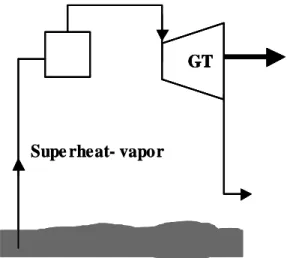
Figure A.4: Direct-intake exhausting to atmosphere turbine.
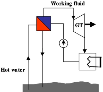
If the geothermal well produces hot water instead of steam, electricity can be still generated by means of binary cycle plants, fig. A.5. These plants operate with a secondary, low boiling point working fluid, (Freon, ammonia, isobutene, etc) in a thermodynamic cycle known as the organic Rankine cycle. The working fluid is vaporized by the geothermal heat. The vapour expands as it passes through the organic
GT
Supe rheat- vapor GT GT GT
Appendix A. Some consideration about thermodynamic indicators for renewable energies
222
vapour turbine, which is coupled to the generator. The exhaust vapor in subsequently condensed in a water cooler condenser and is recycled to the vaporiser by a pump3.
Figure A.5: The binary geothermal power cycle.
Accordingly, the second law efficiency for the binary geothermal power cycle can be described as follow: − + − − = η ) p p ( v T T ln T C ) T T ( C m W 0 0 0 0 p 0 p . w out II (A.8)
Where mw is the pressurized hot water mass flow, T is the hot water temperature, Cp is
the working fluid specific heat, and p is the hot water pressure. The Subscripts 0 point out the environmental conditions fro each magnitude.
Finally, a number of conclusions can be draw: in order to define efficiencies indicators for renewable energy systems, results for wind, hydro a geothermal plant should be calculated as define above, while for solar or biomass traditional first-law efficiencies ca be applied. GT Working fluid Hot water GT Working fluid Hot water
223
2 Eduards, L.M., Chilingar, G.V., Rieke, H.H., Fertl, W.H., (eds) 1982, “Handbook of Geothermal Energy”
Gulf Publishing Co, Houston, p. 613
3
Barbier, E., 1997, “Nature and technology of geothermal energy: A review” Renewable and Sustainable Energy Reviews, 1, pp. 1-69