Chapter 4
CODES AND NODALIZATIONS
4.1 Introduction
Continuous progresses in numerical modeling, codes developments, and the increase of computational power in the Personal Computers (PC) during the last years, has allowed to perform easily detailed transient calculations for NPP [17]. Moreover, the development of special interface protocols like the Parallel Virtual Machine (PVM) [18], has allowed coupling different types of codes (e.g., thermal-hydraulic, neutron kinetics, for sub-channel analysis) performing more accurate analyses.
The transient analyzed in this thesis, as described in Chapter 3.2, involves great neutron flux redistribution, great values of reactivity insertion and severe temperature conditions for the fuel. Furthermore, performing a complete safety analysis requires understanding the effects on the whole part of the plant too. Until several years ago, this type of safety analysis was executed by thermal-hydraulic codes with point kinetics card for neutron calculations, or using 3D neutron kinetics codes with few nodes, in a stand alone mode, assuming conservative input data and obtaining conservative results.
Nowadays, the needs to execute a best estimate analyses, has directed to the use of the-state-of-the-art coupled codes.
Thus, a coupled 3D neutron kinetics/thermal-hydraulic system code was used, with a 2D neutron transport code for the cross section library generation.
4.2 General overview of the calculation flow
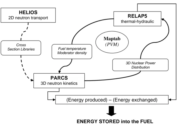
The architecture of the calculations is illustrated in the chart of the figure 4.2.1. The code used for the cross section library generation was the 2D neutron transport code HELIOS (see Chapter 4.3.1); instead, for the transient calculation, it was used the 3D neutron kinetics code PARCS (see Chapter 4.5.1) coupled with the thermal-hydraulic system code RELAP5 (see Chapter 4.4.1). The path followed was this.
Cross section library, after the creation by HELIOS code and after an interpolating and a formatting process performed by an ‘ad-hoc’ FORTRAN program (see Appendix C), were used by PARCS code in the transient calculations.
During these calculations, PARCS sends by a protocol (PVM) and thanks to the coupling file MAPTAB (see Chapter 4.4.2), the information about the 3D power distribution inside the core to the RELAP code. Here, with the correlations established by the MAPTAB file, fuel temperatures and moderator densities are calculated for every fuel assembly, together with all the relevant thermal-hydraulic parameters for the remaining part of the plant described. Thus, updated moderator densities and fuel temperatures are sent again to PARCS by PVM, for perform nuclear calculations for the successive time step.
Fig. 4.2.1 – Calculation Flow
The process is stopped by the reached steady state conditions or by the end of transient time.
As can be seen in the Figure 4.2.1., one of the main outcomes of the transient calculations was the energy stored into the fuel. In fact, as described in Chapter 2.y, this is the main parameter that has to be calculated during a RIA to assess the damage of the fuel. This is not a value automatically calculated by the codes, so the developing of an appropriate procedure was necessary.
It was created an ‘ad-hoc’ FORTRAN program that, analyzing the PARCS code output file, extracted the power of an indicated FA, calculating thank an integral operation the energy produced for every time step. In the RELAP5 code, instead, there were created ‘ad-hoc’ control variables, in order to obtain, after the transient execution, the energy exchanged by a FA with the coolant. Utilizing these two calculated parameter (energy produced and energy exchanged) in a successive commercial program for data processing (ORIGIN 5.0) it was finally possible to obtain the energy stored into the fuel for every time step and its maximum value.
4.3 Neutron cross section generation
4.3.1 Cross section generator code overview
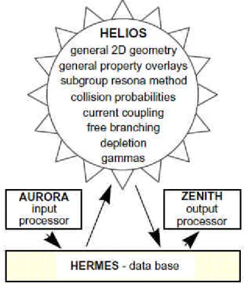
HELIOS is a neutron and gamma transport code for lattice burnup, in general two-dimensional geometry. It was developed by Studsvik™ ScandPower since the 1993[19]. The last code version (the HELIOS-1.6), released in April 2000, was used. As can be seen in Figure 4.3.1.1, HELIOS is composed by several modules. In particular, there are:
- AURORA, the input processor code module - ZENITH, the output processor code module
The data flow between these codes is via a data base that is accessed and maintained by the subroutine package HERMES.
HELIOS 2D neutron transport code PARCS 3D neutron kinetics code RELAP5 thermal-hydraulic code
(Energy produced) – (Energy exchanged)
ENERGY STORED into the FUEL Maptab (PVM) 3D Nuclear Power Distribution Fuel temperature Moderator density Cross Section Libraries
Fig. 4.3.1.1 – Data flow between HELIOS and its input/output processors AURORA/ZENITH
AURORA reads and processes and then saves the User’s input. The result is a number of "User arrays". These arrays, information on their sizes, and the User’s input, are written into a HERMES data base for retrieval by HELIOS and/or ZENITH.
For each case HELIOS retrieves the input from this data base and executes the calculations specified therein.
The type and amount of the output depends on what has been specified by the user in the input. This output is a number of "ZENITH arrays" that start on the letter "Z", which are written into the same data base for retrieval and further processing by ZENITH.
The AURORA input file consists of the following data types:
• the nuclear-data library with the basic nuclear data, which also defines the energy discretizations (group structures) of the particles (neutron and gamma) transport calculations;
• data that define the (initial) number densities of materials, and the elements of the albedo matrix elements;
• data that define the geometry of the system, including the spatial and angular discretizations to be used in the transport calculations;
• data that assign one or more property sets to the geometric system, thus defining one or more "states" of that system;
• data that define the execution sequence of the calculations; • data that define what output will be saved in the data base;
• optional data that define an experimental buckling, change default iteration parameters, accuracies and methods, and produce outputs.
At each calculational point (also called reactivity point), the essential results are particle fluxes and currents, and in case of a burnup or a time step, the new material number densities. Together with the nuclear-library data and the user's input, this is all that is needed to obtain an output. It is, however, not feasible to save at each calculational point, in all energy groups and all regions, fluxes,
number densities and isotopic resonance-shielded cross-sections or, in all energy groups and at all interfaces, the currents in all angular sectors. Therefore, the user has to define in the input what output must be saved in the data base. For example, two-group homogenized data of a fuel assembly, one-group fluxes and macroscopic energy-production cross sections, κΣf, for all the fuel pins (to obtain power maps), et cetera.
HELIOS consists of a main module (LINK00), which calls nineteen computational modules, LINK01-11 and LINK13–20. The first eleven take care of the input treatment, they are called once per case. Then, the other eight take care of the calculations and of the saving and the formatting of the data. The following is a very brief description of the tasks/contents of each of the modules of HELIOS (LINK12 does not exist):
LINK00: It starts the calculations, initiates the files and calls the modules.
LINK01: It reads and rearranges some basic library data. It can also evaluate subgroup constants for the resonance calculations
LINK02: It locates the next case in the HERMES data base, sets dimensioning data and options that come from AURORA, and estimates dimensioning data for the geometry treatment. It also contains the subroutines that interact with the HERMES data base.
LINK03: It sets up the calculational path.
LINK04: It interprets the geometric input structures
LINK05: It builds up the geometric system from the structures
LINK06: If specified in the input, structures can be fused by this module into space elements, LINK07: It interprets the overlay input to define one or more overlay sets for materials, temperatures and density-correction factors.
LINK08: It interprets material and albedo input.
LINK09: It sets up administrative arrays for the output treatment, and creates in the HERMES data base those catalog chains and output data lists that do not depend on the reactivity points
LINK10: It analyses the space-element types for symmetries to be used in the first-flight-probability calculations
LINK11: It draws in each space-element type the chords for the evaluation of the first-flight probabilities
LINK13: In the first stage, it prepares cross sections for the current-coupling-collision-probabilities (CCCP) calculations from which the equivalence cross sections are determined. In the second stage, it evaluates the effective resonance cross sections and the modified out-scattering cross sections due to the flux dip.
LINK14: It sets up the macroscopic neutron or gamma cross sections of the regions. For the gamma calculations, it also determines the sources in the regions from neutron fluxes and the microscopic (neutron, gamma) matrices in the library.
LINK15: It evaluates, per space element and per group, first-flight probabilities for the calculations of the resonance, neutron, or gamma fluxes. It converts these probabilities into response fluxes, and multiple-flight transmission and escape probabilities, which are used in the CCCP iteration process. LINK16: It solves the fluxes and partial currents of the particles according to the CCCP method described. It also contains the subroutine that obtains from the particle balance the net leakage in all groups and regions.
LINK17: It uses the B1 method to evaluate the criticality (or leakage) spectrum of the neutron flux. It enforces this spectrum on the neutron flux obtained from the CCCP method.
LINK18: It does the burnup calculations using a predictor-corrector method. The basic results are the burnup of the individual materials, their new number densities and the time-averages of these number densities during the actual burnup step.
LINK19: It saves number densities and other information for restart calculations. These data are dumped (saved) as data lists in a HERMES data base.
LINK20: It processes the data to obtain the user-specified output. These results are saved as data lists in the I/O HERMES data base.
4.3.2 Neutron cross section modeling
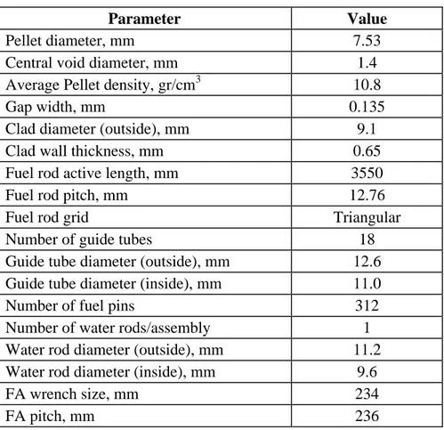
In Figure 4.3.2.1 is illustrated the geometrical and material modeling used for the 1/6th of a FA description. The geometric parameters adopted are reported in the Table 4.3.2.1. They are as far as possible equals to those defined by the vendor in Table 3.1.3.2.
Fig.4.3.2.1 – 1/6th FA cross area – HELIOS modeling
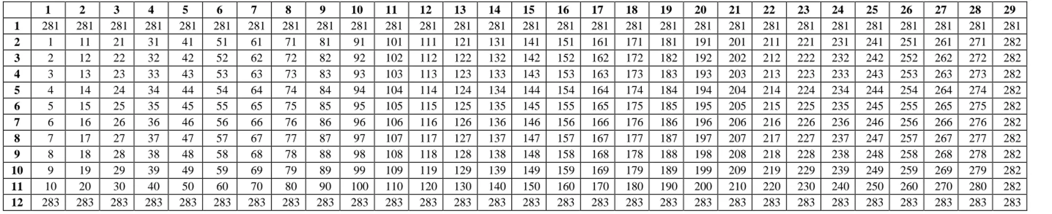
Therefore, for a complete core description, 280 different fuel types were needed (numbered from 1 to 280), together with a 3 ‘special’ fuel type for the reflector description (numbered from 281 to 283) and further 110 different fuel types to describe the FA of the core that could have the rod inserted. In Table 4.3.2.2 is reported the axial composition of every 29 FA type.
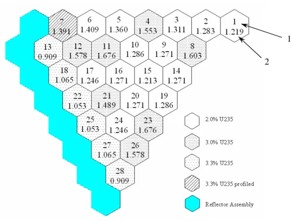
Each fuel type composition, belonging, as indicated in Table 4.3.2.2, to a particular FA, was characterized by the material properties (235U enrichment) and by the burnup. In the Figures 4.3.2.3 to 4.3.2.5 these parameters are showed for BOL and EOC fuel. The core of the WWER reactor was described using a 1/6th symmetry too; thus, it was possible to identify 28 different FA types (see Figure 4.3.2.2). Then, every FA was divided by 10 layers, in order to reconstruct the different burning of the fuel as function of its height, for the BOL and the EOC. Special input file were developed for describing radial, upper and lower reflector too (FA type 29).
Table 4.3.2.1 – FA geometric properties
Parameter Value
Pellet diameter, mm 7.53
Central void diameter, mm 1.4
Average Pellet density, gr/cm3 10.8
Gap width, mm 0.135
Clad diameter (outside), mm 9.1
Clad wall thickness, mm 0.65
Fuel rod active length, mm 3550
Fuel rod pitch, mm 12.76
Fuel rod grid Triangular
Number of guide tubes 18
Guide tube diameter (outside), mm 12.6 Guide tube diameter (inside), mm 11.0
Number of fuel pins 312
Number of water rods/assembly 1
Water rod diameter (outside), mm 11.2 Water rod diameter (inside), mm 9.6
FA wrench size, mm 234
FA pitch, mm 236
Table 4.3.2.1 – Compositions number in axial layers for each assembly type 1 2 3 4 5 6 7 8 9 10 11 12 13 14 15 16 17 18 19 20 21 22 23 24 25 26 27 28 29 1 281 281 281 281 281 281 281 281 281 281 281 281 281 281 281 281 281 281 281 281 281 281 281 281 281 281 281 281 281 2 1 11 21 31 41 51 61 71 81 91 101 111 121 131 141 151 161 171 181 191 201 211 221 231 241 251 261 271 282 3 2 12 22 32 42 52 62 72 82 92 102 112 122 132 142 152 162 172 182 192 202 212 222 232 242 252 262 272 282 4 3 13 23 33 43 53 63 73 83 93 103 113 123 133 143 153 163 173 183 193 203 213 223 233 243 253 263 273 282 5 4 14 24 34 44 54 64 74 84 94 104 114 124 134 144 154 164 174 184 194 204 214 224 234 244 254 264 274 282 6 5 15 25 35 45 55 65 75 85 95 105 115 125 135 145 155 165 175 185 195 205 215 225 235 245 255 265 275 282 7 6 16 26 36 46 56 66 76 86 96 106 116 126 136 146 156 166 176 186 196 206 216 226 236 246 256 266 276 282 8 7 17 27 37 47 57 67 77 87 97 107 117 127 137 147 157 167 177 187 197 207 217 227 237 247 257 267 277 282 9 8 18 28 38 48 58 68 78 88 98 108 118 128 138 148 158 168 178 188 198 208 218 228 238 248 258 268 278 282 10 9 19 29 39 49 59 69 79 89 99 109 119 129 139 149 159 169 179 189 199 209 219 229 239 249 259 269 279 282 11 10 20 30 40 50 60 70 80 90 100 110 120 130 140 150 160 170 180 190 200 210 220 230 240 250 260 270 280 282 12 283 283 283 283 283 283 283 283 283 283 283 283 283 283 283 283 283 283 283 283 283 283 283 283 283 283 283 283 283
Figure 4.3.2.3 – Assembly type map at BOL for 1/6th of the core
Figure 4.3.2.4 – Assembly type map at EOC for 1/6th of the core
1 – FA type
2 – Burnup MWd/KgU
2 1
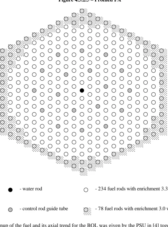
Figure 4.3.2.5 – Profiled FA
- water rod
- control rod guide tube
- 234 fuel rods with enrichment 3.3 w/o
- 78 fuel rods with enrichment 3.0 w/o
The burnup of the fuel and its axial trend for the BOL was given by the PSU in [4] together with the cross section library for the BOL. Instead, the burnup of the fuel and its axial trend for the EOC was given by the Kozloduy 6 NPP and it is reported in Appendix A.
Two neutron energy groups and six decay groups for delayed neutrons were modeled in each cross section library. The first neutron energy group condensed all the neutrons having energies comprised between +8 and 0.625 eV; the second group, instead, condensed all neutrons having energies comprised between 0.625 eV and zero. A fuel composition is described, for each energy group, by:
• Diffusion Coefficient Table • Absorption Cross-Section Table • Fission Cross Section Table (Sf)
• Neutron Fission Cross Section Table (nSf)
• Xenon Absorption Cross Section Table (only for Group 2) • Inverse neutron velocities
• Delayed neutron fraction (only for ‘XSec_20_Beta’ library)
Each table is calculated as a function of the fuel temperature and moderator density. The assembly discontinuity factors (ADF) are taken into consideration implicitly by incorporating them into the cross section (i.e. by dividing the cross sections with ADF for each energy group).
4.3.3 Cross Section Libraries
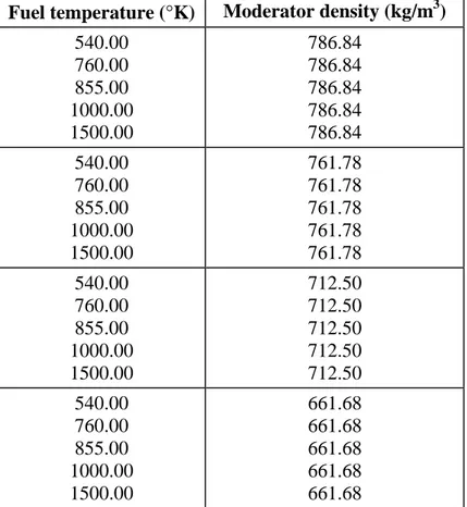
In Tables 4.3.3.1 and 4.3.3.2 are reported the values of the fuel temperature and moderator density (reference points) used for the plotting of the cross section tables. Their combination number (fuel temperature points number * moderator density points number) could be seen as a ‘resolution’ for the cross section library: the greater is this value, the stricter will be the cross section resulted by an interpolation of the cross section library. In this thesis, the entire cross section library except one was calculated with a 20 reference resolution points.
Table 4.3.3.1 – Range of variables for Cross Section Library – 20 reference points
Fuel temperature (°K) Moderator density (kg/m3
) 540.00 760.00 855.00 1000.00 1500.00 786.84 786.84 786.84 786.84 786.84 540.00 760.00 855.00 1000.00 1500.00 761.78 761.78 761.78 761.78 761.78 540.00 760.00 855.00 1000.00 1500.00 712.50 712.50 712.50 712.50 712.50 540.00 760.00 855.00 1000.00 1500.00 661.68 661.68 661.68 661.68 661.68
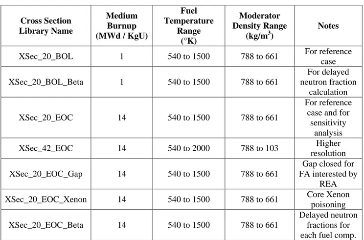
In table 4.3.3.3 are reported the list of Cross Section developed. They were used for reference case and sensitivity analysis calculations (see Chapter 5). For quickly identify the cross section library characteristics, it was adopted the following acronym: “XSec_yy_xxx_part”, where:
- ‘yy’ indicates the number of reference points of a library
- ‘xxx’ indicates if the cross section library describe nuclear fuel at BOL or EOC - ‘part’ not always present, characterize a specific library
For a better understanding, here below it is reported a briefly description of the libraries reported in Table 4.3.3.3:
• XSec_20_BOL is modeling nuclear fuel at the BOL; it was created following the burnup values used for the WWER-1000 CT-1 benchmark of the OECD/NEA [4]
• XSec_20_BOL is modeling nuclear fuel at the BOL; moreover, this library specify for each of the 280 fuel compositions 6 delayed neutron group fractions
• XSec_20_EOC is modeling nuclear fuel at the EOC; it was created following the burnup measurements given by Kozloduy-6 NPP (see Appendix A)
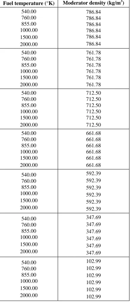
• XSec_42_EOC is modeling nuclear fuel at the EOC, having 42 ‘reference points’. They are reported in Table 4.3.3.2
• XSec_20_EOC_Gap is modeling nuclear fuel at the EOC. It is composed by 280 fuel compositions equal to those used in XSec_20_EOC, plus further 10 fuel compositions modeling the gap closure for the FA where it is assumed to experience the rod ejection. In Table 4.3.3.4 are reported the modified geometrical and physical parameters.
Table 4.3.3.4 – Modified pin values for XSec_20_EOC_Gap
Parameter Value (mm)
Centre void diameter 0.0
Pellet Diameter 7.8
Gap width 0.0
Fuel Density 9.6
• XSec_20_EOC_Xenon is modeling nuclear fuel at the EOC and the core Xenon poisoning. Using a previous HELIOS calculation for obtain the average thermal neutron flux, the time for the Xenon maximum concentration was calculated with the following formula:
Φ
+
+
−
−
−
=
Xe I Xe Xe Xe I Xe I Xe It
λ
λ
σ
λ
γ
γ
λ
λ
λ
λ
ψ)
)(
(
1
ln
1
) (max where- lXe = 2.10*10-5 s-1 is the 135Xe decay constant
- lI = 2.88*10-5 s-1 is the 135I decay constant
- gXe = 0.002 is the 135Xe yield per fission
- gI = 0.061 is the 135I yield per fission
- F = 2*1014 neutron / (cm2 s) is the average thermal neutron flux - sXe = 3*10-18 cm2 is the Xenon absorption cross section
- y is the poisoning coefficient, or the ratio between the thermal neutron captured by the Xenon and those captured by the fuel
and resulted to be roughly 10hours. Then, thanks to an HELIOS feature, there was calculated the cross section value for 280 fuel composition assuming that these experienced a Xenon buildup for a time equal to this previously calculated. A further 10 fuel compositions, which were modeling the FA that experience the rod ejection, were calculated as those of XSec_20_EOC library.
• XSec_20_EOC_Beta is modeling nuclear fuel at the EOC. Moreover, this library specifies for each of the 280 fuel compositions 6 delayed neutron group fractions.
Table 4.3.3.2 – Range of variables for Cross Section Library – 42 reference points
Fuel temperature (°K) Moderator density (kg/m3
) 540.00 760.00 855.00 1000.00 1500.00 2000.00 786.84 786.84 786.84 786.84 786.84 786.84 540.00 760.00 855.00 1000.00 1500.00 2000.00 761.78 761.78 761.78 761.78 761.78 761.78 540.00 760.00 855.00 1000.00 1500.00 2000.00 712.50 712.50 712.50 712.50 712.50 712.50 540.00 760.00 855.00 1000.00 1500.00 2000.00 661.68 661.68 661.68 661.68 661.68 661.68 540.00 760.00 855.00 1000.00 1500.00 2000.00 592.39 592.39 592.39 592.39 592.39 592.39 540.00 760.00 855.00 1000.00 1500.00 2000.00 347.69 347.69 347.69 347.69 347.69 347.69 540.00 760.00 855.00 1000.00 1500.00 2000.00 102.99 102.99 102.99 102.99 102.99 102.99
Table 4.3.3.3 – Cross Section library used Cross Section Library Name Medium Burnup (MWd / KgU) Fuel Temperature Range (°K) Moderator Density Range (kg/m3) Notes
XSec_20_BOL 1 540 to 1500 788 to 661 For reference
case XSec_20_BOL_Beta 1 540 to 1500 788 to 661 For delayed neutron fraction calculation XSec_20_EOC 14 540 to 1500 788 to 661 For reference case and for
sensitivity analysis
XSec_42_EOC 14 540 to 2000 788 to 103 Higher
resolution
XSec_20_EOC_Gap 14 540 to 1500 788 to 661
Gap closed for FA interested by
REA
XSec_20_EOC_Xenon 14 540 to 1500 788 to 661 Core Xenon
poisoning
XSec_20_EOC_Beta 14 540 to 1500 788 to 661
Delayed neutron fractions for each fuel comp.
4.4 3D neutron kinetics calculation 4.4.1 3D neutron kinetics code overview
PARCS is a 3D neutron kinetics code developed for the US-Nuclear Regulatory Commission (NRC) by the Purdue University [20] since the 1998. The version used for the calculations in this thesis was the latest released at that time (PARCS 2.5, September 2003).
PARCS is a three-dimensional (3D) reactor core simulator which solves the steady-state and time-dependent neutron diffusion equation to predict the dynamic response of the reactor to reactivity perturbations such as control rod movements or changes in the temperature/fluid conditions in the reactor core. The code is applicable to both PWR and BWR cores loaded with either rectangular or hexagonal FA. The neutron diffusion equation for the hexagonal FA can be solved for any number of neutron energy group; in this thesis, for the transient calculations, as well as for cross section library, it was always used a two energy group modeling.
Neutronically, the coarse mesh finite difference (CMFD) formulation is employed in PARCS to solve for the neutron fluxes in the homogenized nodes. The triangle-based polynomial expansion nodal (TPEN) method is used in hexagonal geometry to solve the two-node problems for accurate resolution of coupling between nodes in the core [21].
The major calculation features in PARCS include the ability to perform eigenvalue calculations, transient (kinetics) calculations, Xenon transient calculations, decay heat calculations, pin power calculations, and adjoint calculations.
The solution of the CMFD linear system is obtained using a Krylov subspace method which utilizes a BILU3D preconditioner [20] in rectangular geometry and a point ILU preconditioner in hexagonal geometry. The eigenvalue calculation to establish the initial steady-state is performed using the
Wielandt eigenvalue shift method. The pin power calculation method employs a reconstruction scheme in which predefined heterogeneous power form functions are combined with a homogeneous intranodal flux distribution. The homogeneous flux shape is obtained by solving analytically a two-dimensional boundary fixed source problem consisting of the surface average currents specified at the four boundaries.
4.4.2 3D neutron kinetics modeling
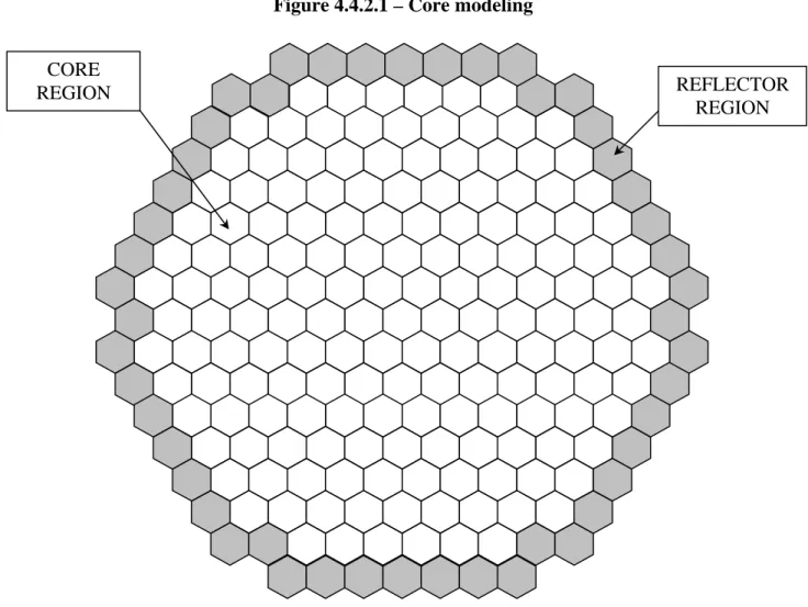
The reactor core was divided in two regions: the active core region and the reflector region (see Fig. 4.4.2.1). There were modeled all the 163 FA of the active core plus 48 ‘reflector’ assemblies for a grand total of 211 assemblies. Sixty-one of the 163 FA were considered ‘rodded’ FA, to model their capacity of hosting a CR cluster (see fig 3.1.4.1 for the disposition).
Twenty-nine or thirty type of assembly (see fig.4.3.2.2), depending by the transient type calculation, were used to describe the different physical composition of the core. Every assembly was divided axially by 22 layer, the first and the last having an height of 0.236 m while the other 20 having an height of 0.1765 m. The first and last portion of the assembly simulates the upper and the lower axial reflector.
Code options for decay heat and Xenon/Samarium calculation during all transient simulated were activated. Cross section libraries generated by HELIOS, after an interpolating and formatting process (see Appendix C) were also put in the code input file. The energy release per fission for the two prompt neutron groups was fixed at 0.3213*10-10 and 0.3206*10-10J/fission.
Figure 4.4.2.1 – Core modeling
REFLECTOR REGION CORE
A total of 4642 neutronic nodes were finally used for the calculations. In Tables 4.4.2.1, 4.4.2.2 are reported the six delayed neutron group fraction used for the calculation with fuel at the BOL and at EOC. The values for the BOL and for the EOC were obtained from the XSec_20_BOL_Beta and from the XSec_20_EOC_Beta library, developing an ‘ad-hoc’ FORTRAN program (see Appendix C) that utilizing the delayed neutron fractions reported there for every fuel composition, performed a flux core averaging with the following operation:
)
6
,....
1
(
2720 1 2720 1=
≅
=
∑
∑
∫
∫
= =i
V
V
dV
dV
j j j j j j ij th th i iφ
φ
β
φ
φ
β
β
where:bi is the i-th fraction of the delayed neutrons group
Fj is the neutron flux at the beginning of the transient in the j-th volume
Vj is the j-th volume of the core
Table 4.4.2.1 – Decay constant and fractions of delayed neutrons for BOL fuel
Delayed neutron group Mean life (l
-1
) (s)
Relative fraction of delayed neutrons (%) 1 80 0.0221 2 32.78 0.1197 3 9.09 0.1161 4 3.27 0.2696 5 0.88 0.1220 6 0.33 0.0504
Total fraction of delayed neutrons: 0.702%
Table 4.4.2.2 – Decay constant and fractions of delayed neutrons for EOC fuel
Delayed neutron group Mean life (l
-1
) (s)
Relative fraction of delayed neutrons (%) 1 80 0.0167 2 32.78 0.0987 3 9.09 0.0912 4 3.27 0.2094 5 0.88 0.1012 6 0.33 0.04
4.5 Thermal-hydraulics calculations 4.5.1 Thermal-hydraulic code overview
The RELAP5 computer code is a light water reactor transient analysis code developed mainly by the Idaho National Engineering Laboratory (INEL) for the U.S. Nuclear Regulatory Commission (NRC) for use in rulemaking, licensing audit calculations, evaluation of operator guidelines, and as a basis for a nuclear plant analyzer. It can be used or the analysis of any kind of transient in LWR. The development of the code began during the seventy years of the last century and continued until nowadays. The version used for the calculations of this thesis is the RELAP5-MOD3.3, the latest released until now [22].
The code is based upon the solution of six partial differential equations that are coupled with (or that need for their solution):
- a wide range ‘Heat Transfer Surface’ for the determination of the Heat Transfer Coefficient, - the equations for the conduction heat transfer into the solid,
- a variety of constitutive equations (e.g. interfacial drag),
- a variety of ‘external models’ (e.g. two phase critical flow, pump, separator), - the equations for ‘tracking’ various non condensable gases,
- the equation for ‘tracking’ boron into the system, - 0-D neutron kinetics equations.
Material properties are embedded into the code, but can also be supplied by the user. The numerical solution method has been specifically adapted for the code and is based upon the use of semi-implicit finite-difference technique. The thermal-hydraulic model can be classified as ‘porous media’ type, to distinguish it from the ‘open media’ that is typical of Computational Fluid Dynamics (CFD) models. The code is capable to model the primary and secondary circuits of NPP as well as all the components belonging to the BOP including the related actuation logic.
The code is classified as a one-dimensional (1-D) code, though ‘fictitious’ 3-D nodalizations can be set-up to simulate three-dimensional flow configurations in open zones. For instance, the core of a NPP can be simulated by several (actually up to a few hundreds) parallel nodes inter-connected ad different axial elevations by ‘cross-junctions’.
4.5.2 Thermal-hydraulic modeling
The nodalization used for transient calculation was a modification of a nodalization previously developed for WWER-1000 reactor by the University of Pisa-DIMNP. The sketch of this nodalization is showed in the Figure 4.5.2.1. It models the whole primary side (RPV, all the four cooling circuit with their SG and MCP, and the ECCS) and the secondary side of the plant until the turbine. The nodalization was qualified as far as possible at the University of Pisa.
The main efforts of this thesis work were aimed to increase the details of the core nodalization, in order to obtain best estimated calculations. The previous nodalization described the core through 29 independent thermal-hydraulic channels, 28 describing the FA channels and one describing the core by-pass. Thus, every thermal-hydraulic channel was modeling six FA.
This kind of approach was unacceptable for a REA study; in fact, this transient violates the 1/6th core symmetry, involving a great neutron flux redistribution and consequently different thermal-hydraulic behavior in the core regions. Therefore, a more detailed nodalization of the part of the core interested by the rod ejection was developed. Each FA where it was postulated to happen the rod ejection and their neighbors FA where modeled on RELAP5 through a single thermal-hydraulic channel (see Figure 4.5.2.2). In this way, it resulted an accurate thermal-hydraulic description of the 1/6th of the core more interested by the accident.
The main modifications of the core nodalization are here briefly resumed: • addition of branches 187 and 188 to the LP 171
• creation of 13 independent thermal-hydraulic channels (281 to 189, 172 to 174 & 130) • addition of branches 195 and 197 to the UP 142
• new assignment of the mass flow for all the core channels and for all the branches • new assignment of the heat exchange surfaces for the all core structures
The resulting core structure was composed of 41 thermal-hydraulic channels, with 14 of these modeling a single FA. An accurate thermal-hydraulic description of the core region more interested by the accident was hence reached. In the figure 4.5.2.2 it can be seen the
Figure 4.5.2.2 – Core layout
\ FA with single thermal-hydraulic channel marked by an hatch FA where postulated REA happens
Figure 4.5.2.3 – Core nodalization sketch 5 4 4 184 2 2 186 3 1 196 129 1 4 5 4 174 173 172 289 188 1 2 5 4 197 3 3 2 1 287 286 285 284 283 282 281 288 187 1 2 4 5 6 7 8 9 195 3 3 2 5 6 7 8 9 1 171 1 1 1 1 132 LP UH bypass to 190 CR guide tube to 142 128 127 126 125 122 118 113 6 5 3 2 9 9 9 9 8 7 8 7 8 7 8 7 6 6 6 5 2 5 2 5 2 3 3 3 3 3 3 4 3 194 193 192 191 9 8 7 6 5 2 1 4 9 8 7 6 5 2 1 9 8 7 6 5 2 1 9 8 7 6 2 1 183 182 181 20 19 18 17 16 15 14 13 12 11 10 9 8 7 6 5 4 3 2 1 130 106 107 111 112 117 121 124 105 110 115 116 119 120 123 114 109 108 104 103 102 101
4.6 Coupling process
Sets of routines implemented in both PARCS and RELAP5 codes, allow to perform data transformation between the different meshes (“Data Mapping”) of the respective codes, with their own dispositions in memory. This is done by using “vectors”, that group all the data to be exchanged, and are transmitted among the codes via standard PVM library.
An intermediate program (GI), built in PARCS and automatically activated, “gets” these vectors, as well as the semaphores of communication and error, “multiplies” them by the permutation matrices for the mesh transformation, and “sends” the product vectors to the other code, also via calls to PVM routines. The differences in thermal-hydraulic and neutronic nodes structure are reported in a special file, called MAPTAB, read by the GI. Here are listed the links between each neutronic node and each thermal-hydraulic node utilized in the system modeling.
Automatic compilation of this mapping file was realized by an ‘ad-hoc’ FORTRAN program, whose functionalities are described in Appendix C.