Chapter 4
On the hybridization of RUFD algorithm with DM for solving multiscale
problems
The Chapter will begin by introducing a general-purpose CEM algorithm, called RUFD (Recursive Update in the Frequency Domain). The advantages of the novel frequency domain scheme over existing techniques in solving EM radiation and scattering problems is investigated in the first part of the chapter.
The central part will be dedicated to the hybridization of the RUFD algorithm with the Dipole Moment method for the solution of multiscale EM problems. Various numerical examples validating the accuracy as well as the numerical efficiency of the method over existing techniques will be presented in the final section.
4.1. The Recursive Update in the Frequency Domain (RUFD) method
Various numerical methods have been developed to numerically solve Maxwell’s equations. Iterative solvers for the discretization of Maxwell’s equations were widely investigated in the framework of the Finite Element Method [62], [63]. In iterative solvers as multigrid techniques a good convergence is often obtained only under certain assumptions, especially if high frequencies have to be resolved [63].
The Finite-Difference Time-Domain method is a well-known numerical algorithm to solve Maxwell’s equations for high frequency problems. However, the standard algorithm, originally proposed by Yee, is limited to isotropic, linear, non-dispersive media [21].
The RUFD method shares some characteristics with the FDTD, though it generates the solution of Maxwell's equations in the frequency rather than in the time domain. The method appears therefore better suited for treating dispersive media, as well as for deriving solutions for problems that involve high-Q structures. Its frequency domain nature renders it more efficient for constructing low-frequency solutions, when compared to the FDTD technique, which requires long run times when an accurate solution is desired at low frequencies [65]. In the method, after the curl operators are replaced by their difference forms, the resulting equations for the electric and magnetic fields are solved in a recursive manner, with no need to solve a matrix equation either iteratively or directly as is the case when the Finite Element Method, for instance, is employed to derive frequency domain solutions of Maxwell’s equations.
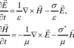
To describe the formulation, let us assume the media is linear and isotropic. The FDTD method is a discretization of Maxwell’s equations for a time periodic source:
1 ˆ ˆ ˆ , 1 ˆ ˆ ˆ j E H E j H E H σ ω ε ε σ ω µ µ ∗ = ∇ × − = − ∇ × − (4.1)
A common method for deriving a stable discretization of (4.1) by means of an iterative solver is to apply the FDTD method and iterate the time stepping.
The time-domain Maxwell’s equations which describe the propagation of EM waves in linear, lossy media read:
1 , 1 E H E t H E H t σ ε ε σ µ µ ∗ ∂ = ∇ × − ∂ ∂ = − ∇ × − ∂ (4.2)
Since a time-periodic source at frequency ω is employed, the solution of (4.2) and (4.1) are related through: ˆ ( ) ˆ ( ) . j t j t E t E e H t H e ω ω = = (4.3)
The FDTD technique discretizes (4.2) in time and space on a staggered grid (see Fig. 4.1).
Figure 4.1. A Unit cell of a staggered grid with depicted locations of the unknowns Ex, Ey, Ez and Hx, Hy, Hz.
4.1. The Recursive Update in the Frequency Domain (RUFD) method 95
derivatives of the curl operator by finite differences:
( 0.5 ) ( 0.5 ) ( ) u u p h u p h p x h ∂ ≅ + − − ∂ (4.4)
The finite difference discretization of Maxwell’s equations is:
1 1/ 2 1 1/ 2 1/ 2 * 1/ 2 1 , 1 , n n n n j n h h h h h E n n n n j n h h h h h H E E H E S e H H E H S e ω τ ω τ σ τ ε ε σ τ µ µ + + + + − + − = ∇ × − + − = − ∇ × − + (4.5)
where ∇ ×h represents the discrete finite-difference curl operator,
(
, , , , ,)
h h x h y h z h h
E = E E E = ∇ ×H and Hh=
(
Hh x, ,Hh y, ,Hh z,)
, τ is the discrete time-step, n h E is the computed electric field at time points nτ, n1/ 2h
H + is the magnetic field at time points (n+1/2)τ, n = 0, 1,... and SE, SH are discrete source terms.
Scheme (4.5) converges to a time periodic solution given particular assumptions [21]. By adding a time-periodic factor to the fields:
1/ 2 ( 1/ 2) ˆ , ˆ , n n j n h h n n j n h h E E e H H e ω τ ω τ − + − + = = (4.6)
leads to the following iteration scheme:
1 1/ 2 / 2 1 / 2 1/ 2 / 2 1/ 2 * 1/ 2 / 2 ˆ ˆ 1 ˆ ˆ , ˆ ˆ 1 ˆ ˆ , j n n n j n j h h h h h E j n j n n n j h h h h h H e E E H e E e S e H e H E H e S ωτ ωτ ωτ ωτ ωτ ωτ σ τ ε ε σ τ µ µ + + + + − − + − = ∇ × − + − = − ∇ × − + (4.7)
that in its explicit form reads:
1 1/ 2 / 2 * 1/ 2 1/ 2 / 2 / 2 ˆ ˆ ˆ /(1 ) , ˆ ˆ ˆ /(1 ) , n n j n j h h h h E n n n j j h h h h H E H e E S e H E H e S e ωτ ωτ ωτ ωτ τ τ τσ ε ε τ σ τ τσ µ µ ε + + − ∗ + − − − = ∇ × + + + = − ∇ × − + + (4.8) If we let ˆ h E , ˆ h
/ 2 / 2 / 2 * / 2 1 ˆ 1 ˆ ˆ , 1 ˆ ˆ ˆ , j j n j h h h h E j j j h h h h H e E H e E e S e e H E H e S ωτ ωτ ωτ ωτ ωτ ωτ σ τ ε ε σ τ µ µ − − = ∇ × − + − = − ∇ × − + (4.9)
which represents a Finite Difference Frequency Domain (FDFD) representation of (4.1). By making τ tend to zero in (4.9), through the well known relationship:
0 1 lim j e j ωτ τ
ω
τ
→ − = (4.10)It is obtained that Eˆh,τ=0 =limτ→0Eˆh( )
τ
and Hˆh,τ=0 =limτ→0Hˆh( )τ
are solution of:, 0 , 0 , 0 * , 0 , 0 , 0 1 ˆ ˆ ˆ , 1 ˆ ˆ ˆ , h h h h E h h h h H j E H E S j H E H S τ τ τ τ τ τ
σ
ω
ε
ε
σ
ω
µ
µ
= = = = = = = ∇ × − + = − ∇ × − + (4.11)meaning that the finite difference solution ˆ , ˆ
h h
E H approximates ˆ ˆE H . ,
Since, in contrast to the Finite Difference Frequency Domain (FDFD) and FEM, the RUFD derives the solution recursively rather than iteratively, it neither suffers from matrix ill-conditioning problems, nor does it require a preconditioner, which is commonly used when solving Maxwell’s equations in the frequency domain. Furthermore, one of the most important advantages of the RUFD method is that it is highly parallelizable, and that it works with a Cartesian mesh, which is simple to generate.
4.1.1. Convergence of the RUFD scheme
To analyze the convergence of iterative scheme (4.7), let us theoretically assume that
, , , 0
ε µ σ σ∗> . Provided the stability assumption:
, 8
h τ ≤ ε µ
(4.12)
then for every ,σ σ∗ it is demonstrated [64] that there exist a τσ σ, ∗independent of h such that the convergence rate of the iterative solver satisfies:
1 ˆ ˆ 1 ( ) : lim ˆ ˆ 1 1 min , 2 n n n E E M E E τ ρ τ σ τ σ ε µ + →∞ ∗ − = ≤ − + (4.13)
4.2. The hybrid DM/RUFD technique 97
for every
, σ σ
τ τ< ∗. It has been proved that for sufficient large σ and σ
*, the method
converges irrespective of the sign of ε and of the mesh-size h. The general scheme reading:
/ 2 / 2 / 2 * / 2 1ˆ 1 ˆ ˆ (1 )(1 ( )) 1 , 2 1 ˆ ˆ ˆ . j j j n h h h h E j j j h h h h H e e sign E H e E S e e H E H e S ωτ ωτ ωτ ωτ ωτ ωτ σ ε τ ε ε σ τ µ µ − − = ∇ × − − − + + − = − ∇ × − + (4.14)
4.2. The Hybrid DM/RUFD technique
The direct solution of multiscale problems by means of conventional CEM methods is highly challenging, even with the availability of modern supercomputers, because of the large number of degrees of freedom introduced when attempting to accurately describe objects with fine features which share the computational domain with objects that are large compared to the operating wavelength.
Hence new numerical techniques for an efficient solution of multiscale electromagnetic problems are highly requested, regardless of the computational CEM method currently being used to tackle them, be it FEM, FDTD or MoM. Dealing with multiscale objects is highly challenging and often forces us to compromise the accuracy (relaxing the numerical discretization process when attempting to capture the small-scale features) in order to cope with the limited available resources in terms of CPU memory and time. In this section, a new scheme that combines the RUFD method with the Dipole Moment method is introduced to solve multiscale problems in a numerically efficient manner [66]. Our objective is to handle the objects with fine features with the DM approach, and not directly with the RUFD, which would require us to use a fine mesh to be handled efficiently (Fig. 4.2).
(a) (b)
Figure 4.2. Conventional solution of a multiscale problem comprising a small object which shares the domain with a large one (a) and DM/RUFD concept (b).
The DM approach begins by representing an object small in terms of wavelengths with an array of electrically small spheres, whose electromagnetic response can be conveniently represented by electric dipole moments [67].
In common with the conventional Method of Moments (MoM), the weight coefficients of the dipole moments are obtained by solving a matrix equation, derived by either imposing the boundary conditions on conducting objects, or by matching polarization currents in the dielectric region (Ch. 3). Once the weights have been derived, the scattered fields inside the domain can be obtained by superimposing the fields radiated by each dipole.
It has been shown that the DM method is very accurate for modeling either dielectric or metallic structures that are small in comparison to the wavelength, be they wire, surface, or volume type of structure, regardless of the radius of the wire, or the thickness of the surface, no matter how small they may be [36], [60].
The main advantage of this hybrid method is that it does not require local mesh refinement for objects with fine features (Fig. 4.2). In fact, the region surrounding the small/thin structure is extracted from the original domain and two different numerical techniques are used for dealing with the two problems.
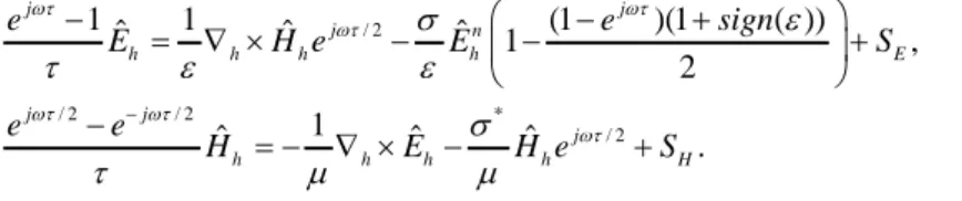
(a) (b) (c)
Figure 4.3. Conventional volume discretization process when dealing with a small structure; (a) extraction of the region surrounding the small object in DM/RUFD technique (b) and discretization of the object in the extracted region with DM (c).
Later, the coupling of the object with the remaining part of the computational domain is achieved by using the fields radiated by the previously extracted region.
Due to this, the presented method does not place a heavy burden on the CPU time and memory as do the conventional approaches when dealing with multiscale problems.
The DM/RUFD method introduced in the following section will be implemented either in an iterative or self-consistent manner.
4.2.1. Iterative DM/RUFD hybrid scheme 99
The proposed method is especially useful for modeling of wire antennas located in the vicinity of inhomogeneous structures, as well as for simulating interconnect structures in integrated circuits, which typically have fine features.
Some numerical experiments demonstrating the performance of the method will be depicted in the final section.
4.2.1. Iterative DM/RUFD hybrid scheme
The hybrid DM/RUFD method has been developed by employing both an iterative and a self-consistent scheme in the contest of electromagnetic scattering. The first algorithm implementation, based on the concept of refining the result at each iteration until a convergence is achieved, turns out to be more accurate and a little more time/memory consuming with respect to the self-consistent one.
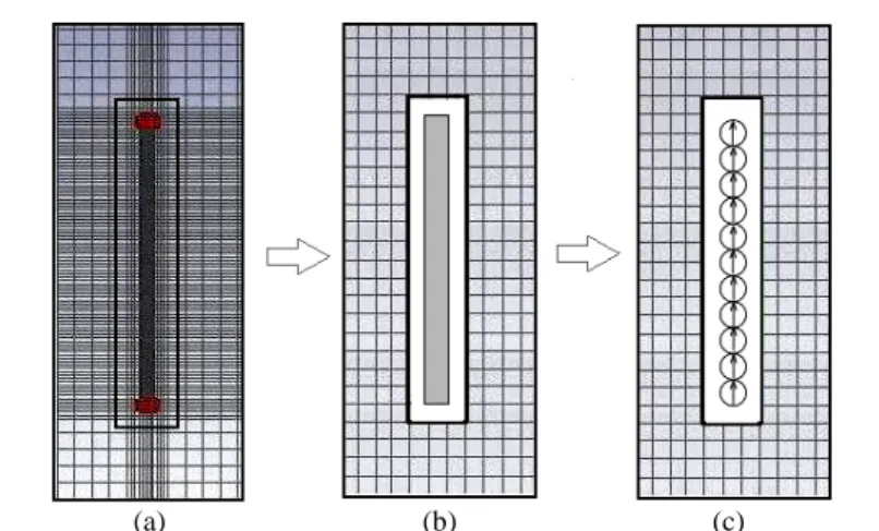
Both implementations begin by extracting from the RUFD domain Σ a region ∂Σ surrounding the small object (for a 2-D representation of the hybrid problem see Fig. 4.4).
Figure 4.4. 2-D representation of a conventional hybrid problem in the RUFD domain comprising a large structure which sits in the vicinity of an electrically small object. A region surrounding the object with small features has been extracted from the original RUFD domain.
Let us assume that two objects, a large PEC plate and a PEC wire small compared to the operating wavelength are located in the RUFD computational domain while a plane wave source starts to propagate on the system.
In the first algorithm iteration the original large problem is solved within the RUFD domain in the absence of the thin structure. This is accomplished by using the original incident plane wave to apply the boundary condition on the large object (e.g., scat inc
tan tan
E = −E if the object is PEC).
In the mean time, the fields scattered by the small structure are derived by using as a source both the original plane wave and the fields scattered from the large structure. The small object is first replaced by an array of spheres (e.g. equivalent dipole moments, see Chapter 3) whose weights need to be determined.
By assuming that there are N spheres, hence N/3N dipoles with unknown dipole moments (in the more general case of a dielectric material 3 dipoles, one for each principal direction need to be considered). By following the notation of Chapter 3, being n
s
Il the dipole moment relating to nth sphere, directed along ˆs; nm,
t s
E being the scattered ˆt component on nth sphere because of ˆs−oriented dipole of mth sphere, namely m
s
Il ; and n, s inc
E be the incident field component at the centre of nth sphere, along ˆs.
A matrix system can be constructed, whose 1st row is expressed, for dielectrics, as in (3.59). The right hand side in the matrix equation of the DM problem (field incident upon each of the constituting dipole moments) is represented by the superposition of both the original plane wave source and the field scattered by the large structure.
These fields are evaluated at the boundary of the extracted region ∂Σ and interpolated to get the N incident fields at each sphere location (see Fig. 4.5 for the example of a wire getting across 4 RUFD cells).
Figure 4.5. A small wire, described by DMs, which extends through 4 RUFD cells. Squares represent dipole moment locations while diamonds represent RUFD field points to be interpolated to get the z-component of the field incident upon each dipole moment.
After solving the matrix system for the weight coefficients of the dipole moments, the scattered field at first iteration inside the domain can be obtained by superposing all dipole moment contributions and the previously derived fields scattered by the large object.
4.2.2. Self-consistent DM/RUFD hybrid scheme 101
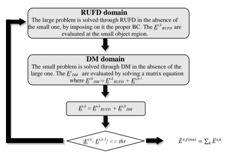
RUFD domain
The large problem is solved through RUFD in the absence of the small one, by imposing on it the proper BC. The Es,k
RUFD are
evaluated at the small object region.
DM domain
The small problem is solved through DM in the absence of the
large one. The Es
DM are evaluated by solving a matrix equation
where Ei,k DM = Es,kRUFD + Es,k-1 Es,k = Es,k RUFD + Es,kDM |Es,k- Es,k-1| <= thr 𝐸�𝑠,𝑓𝑖𝑛𝑎𝑙= ∑ 𝐸�𝑠,𝑘 𝑘
Figure 4.6. Iterative hybrid DM/RUFD scheme flow chart.
At k-th iteration, the same steps are followed, except for the incident plane wave that is replaced by the scattered field derived in the (k-1)-th iteration.
The process is interrupted when the difference between the result at iteration k-th and (k-1)-th is under a given (k-1)-threshold ((k-1)-the algori(k-1)-thm is schematized in Fig. 4.6).
4.2.2. Self-consistent DM/RUFD hybrid scheme
The self-consistent implementation begins as well by extracting from the RUFD domain a region ∂Σ surrounding the small object (Fig. 4.4). This time the whole problem is solved directly by inverting the matrix equation relative to the small problem while the of the large object is brought into the picture by adding contributions to the excitation vector in the DM system.
For this purpose, the impedance matrix Z for the small problem is set up independently of the rest through the DM approach; the right hand side vector for plane wave incidence is computed and stored (we will refer to it as to r.h.s.1).
As a next step the large problem is solved with RUFD in the absence of the thin structure for the original plane wave source. The scattered fields are computed and interpolated at the small object location getting a new excitation vector for the DM system (r.h.s.2).
We assume the current distribution shape for the current is known (we set up one or more macro-basis functions [68]), while the amplitude needs to be determined.
We make radiate the current distribution at the large object location and solve it imposing the boundary condition on its surface (the fields produced by the small object are used as incident field on the large object).
The fields scattered by the large object are computed and interpolated at the small object region getting r.h.s.3. The matrix equation for the small object is set as follows:
1 2 3
Z x= −rhs −rhs −x rhs (4.15) which reflects that the amplitude of the third term on the right hand side still needs to be determined. It is obtained:
3 1 2
(Z+rhs )x= −(rhs +rhs ) (4.16)
The matrix equation is then solved for the weights of the currents x.
The final scattered fields are calculate as a weighted superposition of the three derived contributions as:
, ,1 , 2 ,3
s f s s s
E =E +E +x E (4.17)
A flow chart schematizing the steps followed in the self-consistent scheme is reported in Fig. 4.7. Obviously, being a non-iterative one, the following scheme will result in better performance in terms of run time, while it will be shown to be a bit less accurate in comparison to the iterative hybrid technique in the numerical results section.
The above scheme has been shown to work pretty well when only PEC structures are involved as large objects. When combinations of PEC and dielectrics are involved for the large scatterer, the only application of the boundary condition at the PEC surface has turned out not to be satisfactory in describing the radiation characteristics of the system small object + inhomogeneous scatterer.
4.2.2. Self-consistent DM/RUFD hybrid scheme 103
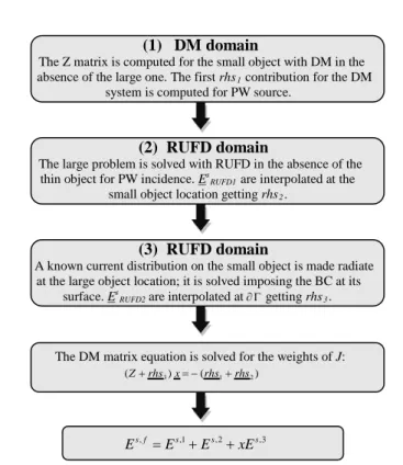
(1) DM domain
The Z matrix is computed for the small object with DM in the absence of the large one. The first rhs1 contribution for the DM
system is computed for PW source.
(2) RUFD domain
The large problem is solved with RUFD in the absence of the thin object for PW incidence. Es
RUFD1 are interpolated at the
small object location getting rhs2.
(3) RUFD domain
A known current distribution on the small object is made radiate at the large object location; it is solved imposing the BC at its surface. EsRUFD2 are interpolated at∂ Γgetting rhs3.
The DM matrix equation is solved for the weights of J: (Z+rhs3)x= −(rhs1+rhs2)
s f, s,1 s,2 s,3
E =E +E +xE
Figure 4.7. Self-consistent DM/RUFD hybrid scheme flow chart.
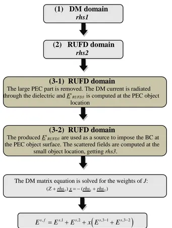
Hence, a modified version of the above scheme, involving the computation of the third excitation contribution (rhs3) in two instead of one step (see Fig. 4.8) has been formulated. In the new scheme the first two DM excitations are calculated as in the previous scheme; the third right hand side contribution is computed by first removing the PEC part and radiating the known small object current through the dielectric at the PEC object location.
As a next step, the previously derived scattered fields are used as a source in the RUFD domain to apply the boundary condition at the PEC object surface. The new rhs3 is represented by the produced scattered fields interpolated at the small object location region. The rest of the procedure remains unchanged.
(1) DM domain rhs1 (2) RUFD domain rhs2 (3-1) RUFD domain
The large PEC part is removed. The DM current is radiated through the dielectric and Es
RUFD3 is computed at the PEC object
location
(3-2) RUFD domain
The produced Es
RUFD3 are used as a source to impose the BC at
the PEC object surface. The scattered fields are computed at the small object location, getting rhs3.
The DM matrix equation is solved for the weights of J: (Z+rhs3)x= −(rhs1+rhs2)
s f, s,1 s,2
(
s,3 1 s,3 2)
E =E +E +x E − +E −
Figure 4.8. Self-consistent modified DM/RUFD hybrid scheme flow chart. The presence of the large object inhomogeneity gives rise to an additional step (3-1) in the scheme.
4.3.1. λ square dielectric-layered conducting plate 105
4.3. Numerical results
In this section some numerical results are presented for plain RUFD algorithm and for the two different hybrid techniques. The numerical efficiency both in terms of run time and memory requirement over existing methods is proved through several scattering examples. Furthermore, the two hybrid techniques are compared both in terms of run time and memory requirements.
4.3.1. λ square dielectric-layered conducting plate
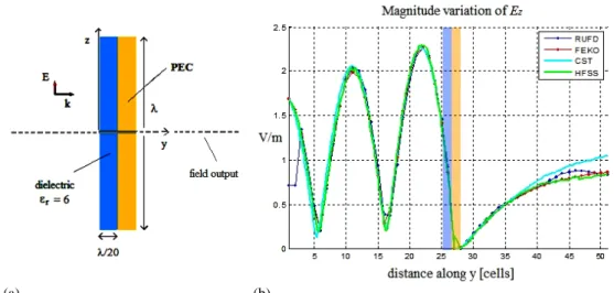
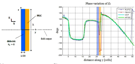
Numerical results for the fields scattered by a dielectric (ε r = 6) layered conducting plate, λ0
on the side under normal plane wave illumination are presented in Figs. 4.9 and 4.10. The magnitude and phase variations of the scattered dominant component are computed varying y (expressed in cells) from 1 to 51.
Perfectly Matched Layer (PML) boundary conditions have been implemented in the code to terminate the computational domain. The results are compared against existing commercial codes implementing different numerical techniques: FEKO (MoM), HFSS (FEM) and CST (Finite Integration Technique (FIT)).
(a) (b)
Figure 4.9. Problem geometry (a) and magnitude variation of scattered Ez (b) computed varying y
along all the computational domain (from cell 1 to cell 51) @ x = y = 0: RUFD results are compared against FEKO, HFSS and CST.
(a) (b)
Figure 4.10. Problem geometry (a) and phase variation of scattered Ez (b) computed varying y along
all the computational domain (from cell 1 to cell 51) @ x = y = 0. RUFD and FEKO, HFSS and CST results are compared.
The discretization for all EM solvers has been kept around λ0/20, while all the simulations
have been carried out on a 4GB RAM and 3.0 GHz intel core 2Duo processor.
The performance in terms of memory requirement and run time are displayed in Table 4.1.
RUFD HFSS FEKO CST Memory requirements (peak) [MB] 301 447.4 860.5 ph: 449.51 vir: 722.84 Simulation time [s] 79.2 132 377.49 215
Table 4.1. The RUFD simulation time and memory requirements are compared against commercial EM solvers HFSS, FEKO and CST.
The RUFD algorithm results to be faster and less memory demanding while compared to different commercial solvers, while keeping the accuracy.
4.3.2. λ square PEC sheet in the presence of a λ/2 conducting wire 107
4.3.2. λ/2 square PEC sheet in the presence of a 3λ/20 conducting wire
Numerical results for the fields scattered by a conducting plate, λ0/2 on the side under
normal plane wave illumination in the presence of a PEC wire which is 3λ/20 in length are presented in Figs. 4.11 and 4.12. The magnitude and phase variations of the scattered dominant component are computed varying y (expressed in cells) from 1 to 51. The PEC sheet is located at cell y = 27 while the wire is located at a distance 0.125λ from the sheet, i.e. 2.5 cells away from the sheet along y. A plane wave source is incident along y with its E-field vector polarized along z.
Absorbing Boundary Conditions (ABC) are used to terminate the computational domain for this simulation. The results in the absence and in the presence of the wire are compared against commercial MoM.
(a) (b)
Figure 4.11. Problem geometry (a) and magnitude variation of scattered Ez (b) computed varying y
along all the computational domain (from cell 1 to cell 51) @ x = y = 0. RUFD and FEKO results are compared.
(a) (b)
Figure 4.12. Problem geometry (a) and phase variation of scattered Ez (b) computed varying y along
all the computational domain (from cell 1 to cell 51) @ x = y = 0. RUFD and FEKO results are compared.
4.3.3. λ square PEC sheet in the presence of a λ/2 conducting wire
The performance both in terms of accuracy and run time of hybrid DMRUFD iterative and self-consistent are evaluated for the numerical example of scattering from a λ on the side PEC sheet and a λ/2 conducting wire. A plane wave is normally incident on the structure with E polarized along z. The relative distance between the sheet and the wire is the same as in the previous example (Fig. 4.12(a)).
The two hybrid schemes are compared in terms of accuracy against existing commercial codes implementing different numerical techniques: FEKO (MoM), HFSS (FEM) and CST (FIT) in Figs. 4.13 and 4.14, while the efficiency of the two hybrid methods is compared in terms of run time and memory requirements in Table 4.2.
The cells size has been kept λ0/20 and PML boundary conditions have been implemented for
simulating both hybrid DM/RUFD cases. All the simulations have been carried out on a Personal Computer with a 4GB RAM and 3.0 GHz intel core 2Duo processor.
4.3.3. λ square PEC sheet in the presence of a λ/2 conducting wire 109
(a) (b)
Figure 4.13. Problem geometry (a) and magnitude variation of scattered Ez (b) computed varying y
along all the computational domain (from cell 1 to cell 51). The results of the hybrid DM/RUFD iterative and self-consistent are compared against commercial MoM, FEM and FIT solvers.
(a) (b)
Figure 4.14. Problem geometry (a) and phase variation of scattered Ez (b). The results of the hybrid
Cell size: λ/20 PML BC Hybrid DM/RUFD Self Consistent Hybrid DM/RUFD Iterative Memory requirements (peak) [MB] 483 481 Simulation time [s] 172.3 601
Table 4.2. The hybrid DM/RUFD iterative and self-consistent implementations are compared in terms of simulation time and memory requirements.
As it can be noted from Figs. 4.13 and 4.14, better performance in terms of accuracy are achieved by using the iterative DM/RUFD hybrid approach while it is apparent from Table 4.2 that the self-consistent approach results faster. The memory requirement is comparable for the two cases.
4.3.4. λ square dielectric-coated PEC sheet in the presence of a λ/2 PEC wire
In the following test example a PEC square sheet coated with λ/10 thick dielectric (εr = 6), which shares the computational domain with a λ/2 in length conducting wire, is invested by a plane wave which propagates along the y-axis with its field vector polarized along z (Fig. 4.15).
(a) (b)
4.3.4. λ square dielectric-coated PEC sheet in the presence of a λ/2 in length PEC wire 111 The problem is solved through scheme 4.8; the real and imaginary parts of some of the computed contributions to the final scattered field are reported in Fig. 4.16.
The final total field distribution computed by the present approach is compared against commercial codes implementing the MoM approach (FEKO), the FEM (HFSS) and the FIT (CST). A satisfactory agreement is achieved against HFSS and CTS both in amplitude and in phase (see Fig. 4.17) while the MoM code gives inaccurate results.
(a) (b)
Figure 4.16. Variation of the real (a) and imaginary parts (b) of contributions from steps 2, 3-1 and 3-2 to the final scattered field.
(a) (b)
Figure 4.17. Magnitude (a) and phase (b) variation of the final total fields along the y-axis. The results computed through the modified self-consistent hybrid scheme are compared against FEKO, HFSS and CST.
The performance in terms of run time and memory requirement are reported in Table 4.3. As can be noted from the Table, the Hybrid DM/RUFD code performs better both in terms of memory and run time against CST and HFSS. The time performance are comparable with the MoM, which gives inaccurate results for this case though.
discretization: ≈ λ/20 Hybrid DM/RUFD
Self-consistent FEKO CST (FD version) HFSS Memory requirements (peak) [MB] 348 690.6 ph: 1590 vir: 1910 1680 Simulation time [s] 260 284.12 1565 1861
Table 4.3. The performance of the hybrid DM/RUFD self-consistent implementation is compared in terms of simulation time and memory requirements against FEKO, CST and HFSS.