4. RESULTS
4.1. Hediste diversicolor
4.1.1. Within-population genetic diversity
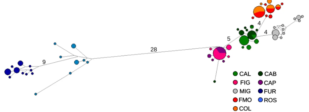
The analysis of the 181 specimens included in this study yielded 544 bp long sequences. A total of 58 haplotypes were detected for a total of 91 polymorphic sites of which 75 were parsimony informative. JModelTest recognised TrN+G (Tamura & Nei, 1993) as the best fitting model of evolution using the Bayesian Information Criterion (BIC). The gamma shape parameter was α = 0.08. the transition/transversion ratio was 30.4 and the mean base composition was 33.5% thymine, 21.0% cytosine, 30.2% adenine and 15.3% guanine. Alignment of aminoacidic sequences revealed a total of 12 non-synonymous mutations at sites 117, 156, 169, 252, 258, 274, 306, 310, 336, 339, 384 and 408. Three of the non-synonymous mutations were shared by the Atlantic samples only (FUR + ROS): 156, 274 and 384.
High levels of haplotype diversity were found at most of the considered localities, as well as the total dataset (Table. 4.1). Smaller values of haplotype diversity were detected for the populations of FIG and CAP. Nucleotide diversity was generally low (Table 4.1), but higher values were found for the populations of MIG and ROS.
Table 4. 1. N: sample size; NH: number of haplotypes; NS: number of polymorphic sites; NM: number of mutations; h: haplotype diversity ±std. dev.; π: nucleotide diversity ±std. dev.
N NH NS NM h π CAL 25 6 5 5 0.627 ±0.101 0.0015 ±0.0003 FIG 22 4 3 3 0.455 ±0.115 0.0009 ±0.0003 MIG 22 11 12 12 0.870 ±0.053 0.0083 ±0.0012 FMO 22 8 5 5 0.792 ±0.069 0.0024 ±0.0004 COL 22 5 4 4 0.701 ±0.079 0.0019 ±0.0003 CAB 21 8 16 16 0.710 ±0.097 0.0037 ±0.0016 CAP 13 4 3 3 0.526 ±0.153 0.0011 ±0.0004 FUR 22 10 13 13 0.866 ±0.046 0.0054 ±0.0007 ROS 12 8 26 26 0.909 ±0.065 0.0139 ±0.0028 Tot 181 58 91 99 0.950 ±0.007 0.0327 ±0.0024
4.1.2. Among-population genetic diversity
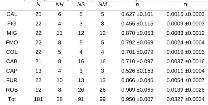
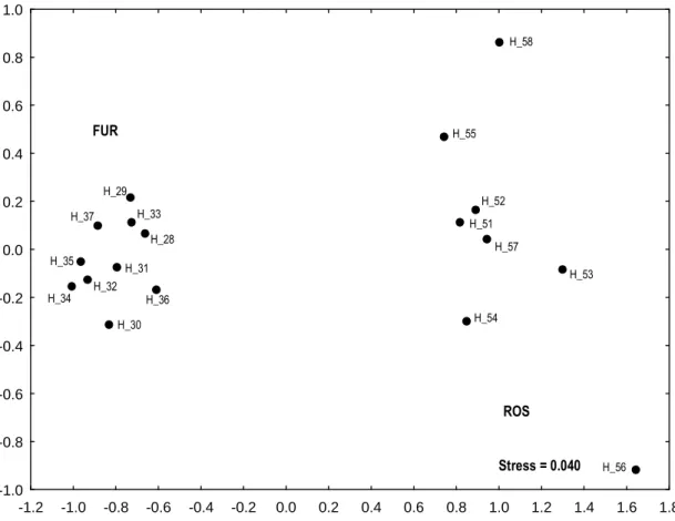
Tamura and Nei (1993) genetic distances among haplotypes of H. diversicolor are reported in Appendix I. The MDS on the total dataset (Fig. 4.1) shows a clear separation of Atlantic and Mediterranean samples along the horizontal axis. In the MDS relative to Atlantic samples only (Fig. 4.2), a haplogroup relative to the FUR population is visible on the left, while haplotypes relative to ROS population are scattered on the right side of the graph. The MDS relative to Mediterranean samples (Fig. 4.3) revealed the presence of five clusters of haplotypes. Two of the clusters shared haplotypes from MIG, one was composed by FMO and COL haplotypes, one by CAB and CAL and the last one by CAP and FIG haplotypes. The haplotype H_8 from CAB was placed alone in the lower left part of the graph, relatively close to the CAP and FIG cluster (Fig. 4.3).
-0.8 -0.6 -0.4 -0.2 0.0 0.2 0.4 0.6 0.8 1.0 1.2 1.4 1.6 -0.015 -0.010 -0.005 0.000 0.005 0.010 0.015 0.020 0.025 0.030 H_31 H_8 H_13 H_14 H_15 H_16 H_17 H_18 H_19 H_56 H_53 H_58 H_55 H_51 H_54 H_52 H_57 H_29 H_33 H_28 H_37 H_36 H_30 H_35 H_32 H_34 H_22 H_23 H_21 H_27 H_39 H_26 H_20 H_38 H_24 H_25 H_5 H_9 H_4 H_12 H_11 H_1 H_7 H_10 H_2 H_3 H_6 H_44 H_41 H_40 H_47H_43 H_49 H_42 H_46 H_48 H_50 H_45 MEDITERRANEAN ATLANTIC Stress = 0.001 -0.8 -0.6 -0.4 -0.2 0.0 0.2 0.4 0.6 0.8 1.0 1.2 1.4 1.6 -0.015 -0.010 -0.005 0.000 0.005 0.010 0.015 0.020 0.025 0.030 H_31 H_8 H_13 H_14 H_15 H_16 H_17 H_18 H_19 H_56 H_53 H_58 H_55 H_51 H_54 H_52 H_57 H_29 H_33 H_28 H_37 H_36 H_30 H_35 H_32 H_34 H_22 H_23 H_21 H_27 H_39 H_26 H_20 H_38 H_24 H_25 H_5 H_9 H_4 H_12 H_11 H_1 H_7 H_10 H_2 H_3 H_6 H_44 H_41 H_40 H_47H_43 H_49 H_42 H_46 H_48 H_50 H_45 -0.8 -0.6 -0.4 -0.2 0.0 0.2 0.4 0.6 0.8 1.0 1.2 1.4 1.6 -0.015 -0.010 -0.005 0.000 0.005 0.010 0.015 0.020 0.025 0.030 H_31 H_8 H_13 H_14 H_15 H_16 H_17 H_18 H_19 H_56 H_53 H_58 H_55 H_51 H_54 H_52 H_57 H_29 H_33 H_28 H_37 H_36 H_30 H_35 H_32 H_34 H_22 H_23 H_21 H_27 H_39 H_26 H_20 H_38 H_24 H_25 H_5 H_9 H_4 H_12 H_11 H_1 H_7 H_10 H_2 H_3 H_6 H_44 H_41 H_40 H_47H_43 H_49 H_42 H_46 H_48 H_50 H_45 MEDITERRANEAN ATLANTIC Stress = 0.001
Fig. 4.1. MDS of the Tamura and Nei (1993) genetic distances on all haplotypes of H. diversicolor. Haplotype codes are as in Appendix II
-1.2 -1.0 -0.8 -0.6 -0.4 -0.2 0.0 0.2 0.4 0.6 0.8 1.0 1.2 1.4 1.6 1.8 -1.0 -0.8 -0.6 -0.4 -0.2 0.0 0.2 0.4 0.6 0.8 1.0 FUR ROS H_56 H_53 H_58 H_55 H_51 H_54 H_52 H_57 H_29 H_33 H_28 H_37 H_31 H_36 H_30 H_35 H_32 H_34 Stress = 0.040 -1.2 -1.0 -0.8 -0.6 -0.4 -0.2 0.0 0.2 0.4 0.6 0.8 1.0 1.2 1.4 1.6 1.8 -1.0 -0.8 -0.6 -0.4 -0.2 0.0 0.2 0.4 0.6 0.8 1.0 FUR ROS H_56 H_53 H_58 H_55 H_51 H_54 H_52 H_57 H_29 H_33 H_28 H_37 H_31 H_36 H_30 H_35 H_32 H_34 -1.2 -1.0 -0.8 -0.6 -0.4 -0.2 0.0 0.2 0.4 0.6 0.8 1.0 1.2 1.4 1.6 1.8 -1.0 -0.8 -0.6 -0.4 -0.2 0.0 0.2 0.4 0.6 0.8 1.0 FUR ROS H_56 H_53 H_58 H_55 H_51 H_54 H_52 H_57 H_29 H_33 H_28 H_37 H_31 H_36 H_30 H_35 H_32 H_34 Stress = 0.040
Fig. 4.2. MDS of the Tamura and Nei (1993) genetic distances on atlantic haplotypes of H.
-1.5 -1.0 -0.5 0.0 0.5 1.0 1.5 2.0 -1.4 -1.2 -1.0 -0.8 -0.6 -0.4 -0.2 0.0 0.2 0.4 0.6 0.8 1.0 CAB + CAL CAP + FIG FMO + COL MIG MIG H_8 H_13 H_14 H_15 H_16 H_17 H_18 H_19 H_44 H_41 H_40 H_47 H_43 H_49 H_42 H_46 H_48 H_50 H_45 H_5 H_9 H_4 H_12 H_11 H_1 H_7 H_10 H_2 H_3 H_6 H_22 H_23 H_21 H_27 H_39 H_26 H_20 H_38 H_24 H_25 Stress = 0.081 -1.5 -1.0 -0.5 0.0 0.5 1.0 1.5 2.0 -1.4 -1.2 -1.0 -0.8 -0.6 -0.4 -0.2 0.0 0.2 0.4 0.6 0.8 1.0 CAB + CAL CAP + FIG FMO + COL MIG MIG H_8 H_13 H_14 H_15 H_16 H_17 H_18 H_19 H_44 H_41 H_40 H_47 H_43 H_49 H_42 H_46 H_48 H_50 H_45 H_5 H_9 H_4 H_12 H_11 H_1 H_7 H_10 H_2 H_3 H_6 H_22 H_23 H_21 H_27 H_39 H_26 H_20 H_38 H_24 H_25 -1.5 -1.0 -0.5 0.0 0.5 1.0 1.5 2.0 -1.4 -1.2 -1.0 -0.8 -0.6 -0.4 -0.2 0.0 0.2 0.4 0.6 0.8 1.0 CAB + CAL CAP + FIG FMO + COL MIG MIG H_8 H_13 H_14 H_15 H_16 H_17 H_18 H_19 H_44 H_41 H_40 H_47 H_43 H_49 H_42 H_46 H_48 H_50 H_45 H_5 H_9 H_4 H_12 H_11 H_1 H_7 H_10 H_2 H_3 H_6 H_22 H_23 H_21 H_27 H_39 H_26 H_20 H_38 H_24 H_25 Stress = 0.081
Fig. 4.3. MDS of the Tamura and Nei (1993) genetic distances on mediterranean samples of H.
Diversicolor. Haplotype codes are as in Appendix II
The presence of genetic structuring in the species was further investigated with an exact test. The null hypothesis of the test is the absence of gnetic structure. The exact probability value after 30000 Markov steps was P < 0.001, permitting to reject the null hypothesis.
Values of Φst calculated between each population pair are reported in Table 4.2, below the diagonal. All calculated values resulted high and highly significant (P < 0.001) except for the COL/FMO comparison. Lower levels of significance (P < 0.05) were found for the CAP/FIG pair. An exact test on Φ-statistics values calculated for each couple of populations was conducted and all calculated values resulted significant after 100000 steps. Results are reported on Table 4.2, above the diagonal.
Table 4.2. Φst values for each couple of populations (below diagonal) and Exact test of
population differentiation based on Φst (Above diagonal).
FIG MIG FMO COL CAB CAP FUR ROS
FIG - *** *** *** *** NS *** *** MIG 0.802*** - *** *** *** *** *** *** FMO 0.919*** 0.697*** - NS *** *** *** *** COL 0.930*** 0.705*** -0.003NS - *** *** *** *** CAB 0.843*** 0.679*** 0.776*** 0.796*** - *** *** *** CAP 0.071* 0.767*** 0.908*** 0.921*** 0.821*** - *** *** FUR 0.959*** 0.922*** 0.952*** 0.955*** 0.940*** 0.951*** - *** ROS 0.913*** 0.867*** 0.911*** 0.915*** 0.887*** 0.887*** 0.727*** -
Three-level AMOVA assigned 77% of molecular variance among groups, 18% among populations, and 5% within populations (Table 4.3).
Table 4.3. Three-level analysis of molecular variance (AMOVA) for 9 populations of H. diversicolor. P-values were calculated after a permutation test with 10,000 replicates
Source of variation df Variance component Percentage of variation Φst P Among groups 1 16.36218 77.35 Φct = 0.773 0.02 Among populations within groups 7 3.71448 17.56 Φsc = 0.775 <0.001 Within populations 172 1.07743 5.09 Φst = 0.94 <0.001
Along with the AMOVA, Φ-statistics values were calculated (Table 4.3). All Φ -statistics values were significantly different from zero after a 10,000 replicates permutation test.
Replicate runs of BAPS yielded identical results and produced six genetic clusters (hereafter called haplogroups I to VI) supported by the maximum probability value (P = 1) (Fig. 4.4). Only two out of 181 individuals (1%) exhibited uncertain assignment (P < 0.05): CAB11 (H_5) and CAB26 (H_8); 149 individuals (82%) were assigned with maximum probability (P = 1). Haplogroup I includes all haplotypes from CAL and CAB with the exception of CAB26 which is the only individual which have
not been assigned to the same haplogroup of other individuals of its population; haplogroup II included all the haplotypes sampled from FIG and CAP and CAB26; haplogroup III included haplotypes from MIG; haplogroup IV included haplotypes from FMO and COL; haplogroup V included haplotypes from FUR and haplogroup VI included all haplotypes from ROS (Fig. 4.4).
I II III IV IV I II V VI
* *
CAL FIG MIG FMO COL CAB CAP FUR ROS
I II III IV IV I II V VI
* *
CAL FIG MIG FMO COL CAB CAP FUR ROS
Fig. 4.4. Assignment probabilities of samples from individual genotypes (bar graphs) among the four regions using Bayesian analysis of population structure (BAPS). Each colour represent a different haplogroup. Haplogroup names are reported on the top of the bar graph. Asterisks on the bar graph
indicate individuals with uncertain assignment (P < 0.05).
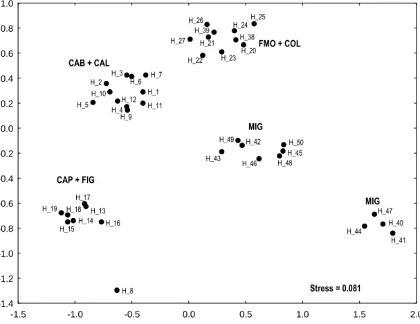
The 181 sequences yielded a network where six main haplogroups can be observed (Fig. 4.5). It is worth noting that these clusters corresponded to the haplogroups detected with Bayesian assignment analysis (Figs 4.4, 4.5).
28 9 5 4 4 CAL FIG MIG FMO COL CAB CAP FUR ROS 28 9 5 4 4 28 9 5 4 4 CAL FIG MIG FMO COL CAB CAP FUR ROS CAL FIG MIG FMO COL CAB CAP FUR ROS
Fig. 4.5. Median-joining network of 181 sequences of H. diversicolor COI. Linkers connecting haplotypes are approximately proportional to the number of mutations. Number of mutations separating the main haplogroups are shown above linkers
The tree obtained by the complete alignment of all haplotypes is visible in Appendix III.
4.1.3. Inferences on demographic history and neutrality tests
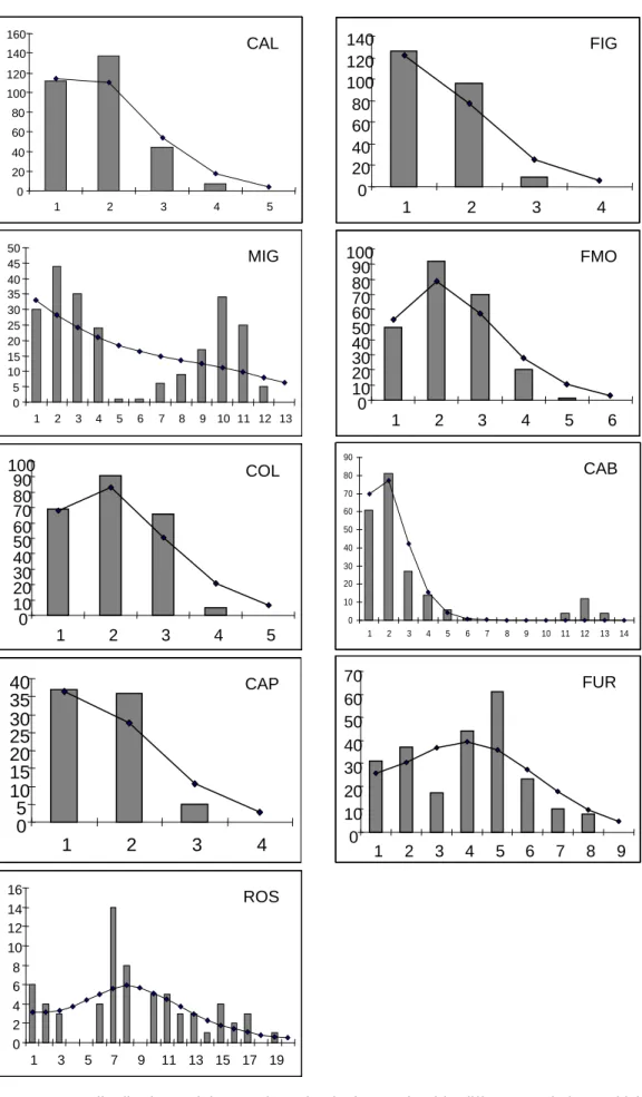
Mismatch distributions obtained for MIG, CAB and FUR are bimodal, they were multimodal for ROS and unimodal for all of the other populations (Fig. 4.6). The sums of squared differences were not significant in all cases (Table 4.4). Values of Harpending’s (1994) raggedness index were not significant (Table 4.4). Values of Tajima’s (1989) D neutrality test were not significant except for CAB, where P = 0.05 (Table 4.4). Fu’s (1997) FS neutrality test gave significant negative values for CAL,
FMO and CAP populations (Table 4.4). Ramos-Onsins & Rozas’ (2002) R2 tests
0 5 10 15 20 25 30 35 40 45 50 1 2 3 4 5 6 7 8 9 10 11 12 13 MIG 0 20 40 60 80 100 120 140 160 1 2 3 4 5 CAL 0 10 20 30 40 50 60 70 80 90 1 2 3 4 5 6 7 8 9 10 11 12 13 14 CAB 0 5 10 15 20 25 30 35 40 1 2 3 4 CAP 0 20 40 60 80 100 120 140 1 2 3 4 FIG 0 10 20 30 40 50 60 70 1 2 3 4 5 6 7 8 9 FUR 0 10 20 30 40 50 60 70 80 90 100 1 2 3 4 5 6 FMO 0 10 20 30 40 50 60 70 80 90 100 1 2 3 4 5 COL 0 2 4 6 8 10 12 14 16 1 3 5 7 9 11 13 15 17 19 ROS 0 5 10 15 20 25 30 35 40 45 50 1 2 3 4 5 6 7 8 9 10 11 12 13 MIG 0 5 10 15 20 25 30 35 40 45 50 1 2 3 4 5 6 7 8 9 10 11 12 13 0 5 10 15 20 25 30 35 40 45 50 1 2 3 4 5 6 7 8 9 10 11 12 13 MIG 0 20 40 60 80 100 120 140 160 1 2 3 4 5 CAL 0 20 40 60 80 100 120 140 160 1 2 3 4 5 0 20 40 60 80 100 120 140 160 1 2 3 4 5 CAL 0 10 20 30 40 50 60 70 80 90 1 2 3 4 5 6 7 8 9 10 11 12 13 14 CAB 0 10 20 30 40 50 60 70 80 90 1 2 3 4 5 6 7 8 9 10 11 12 13 14 CAB 0 5 10 15 20 25 30 35 40 1 2 3 4 CAP 0 5 10 15 20 25 30 35 40 1 2 3 4 0 5 10 15 20 25 30 35 40 1 2 3 4 CAP 0 20 40 60 80 100 120 140 1 2 3 4 FIG 0 20 40 60 80 100 120 140 1 2 3 4 0 20 40 60 80 100 120 140 1 2 3 4 FIG 0 10 20 30 40 50 60 70 1 2 3 4 5 6 7 8 9 FUR 0 10 20 30 40 50 60 70 1 2 3 4 5 6 7 8 9 0 10 20 30 40 50 60 70 1 2 3 4 5 6 7 8 9 FUR 0 10 20 30 40 50 60 70 80 90 100 1 2 3 4 5 6 FMO 0 10 20 30 40 50 60 70 80 90 100 1 2 3 4 5 6 0 10 20 30 40 50 60 70 80 90 100 1 2 3 4 5 6 FMO 0 10 20 30 40 50 60 70 80 90 100 1 2 3 4 5 COL 0 10 20 30 40 50 60 70 80 90 100 1 2 3 4 5 0 10 20 30 40 50 60 70 80 90 100 1 2 3 4 5 COL 0 2 4 6 8 10 12 14 16 1 3 5 7 9 11 13 15 17 19 ROS 0 2 4 6 8 10 12 14 16 1 3 5 7 9 11 13 15 17 19 0 2 4 6 8 10 12 14 16 1 3 5 7 9 11 13 15 17 19 ROS
Fig. 4.6. Frequency distributions of the number of pairwise nucleotide differences (mismatch) between
COI nucleotide sequences for each population. The solid line is the theoretical distribution under the
Table 4.4. Sum of squared differences in mismatch analysis (SSD), Harpending’s (1994) raggedness index (r), Fu’s (1997) FS and Ramos-Onsins & Rozas’ (2002) R2 statistics in populations of H.
diversicolor POP SSD r D FS R2 CAL 0.010NS 0.119NS -1.09073NS -2.52359* 0.085NS FIG 0.241NS 0.160NS -1.03548NS -1.50599NS 0.109NS MIG 0.033NS 0.812NS 1.29284NS -1.71306NS 0.185NS FMO 0.010NS 0.011NS -0.19551NS -3.65803** 0.126NS COL 0.010NS 0.091NS -0.17143NS -0.91576NS 0.128NS CAB 0.012NS 0.085NS -1.99748* -2.02237NS 0.122NS CAP 0.288NS 0.162NS -1.23300NS -1.65789* 0.129* FUR 0.022NS 0.059NS -0.62682NS -2.48373NS 0.101NS ROS 0.037NS 0.066NS -0.54405NS 0.02527NS 0.129NS * P < 0.05, *** P < 0.001, NS = not significant 4.2. Mytilaster minimus
4.2.1. Within-population genetic diversity
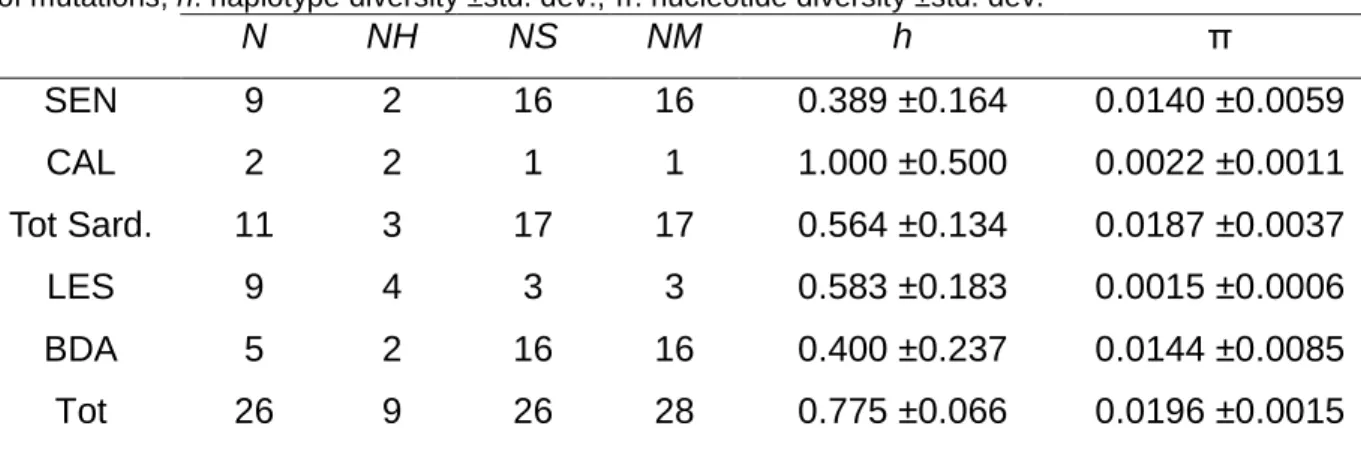
The analysis of the 26 specimens included in this study yielded 445 bp sequences. A total of 9 haplotypes were detected for a total of 26 polymorphic sites of which 16 were parsimony informative. JModelTest by Bayesian Information Criterion recognised HKY (Hasegawa et al., 1985) as the best fitting model of evolution. Transition/transvertion ratio was ti/tv = 3.8 and the mean base composition was 29.9% thymine, 16.5% cytosine, 27.3% adenine and 26.3% guanine. Levels of haplotype diversity, as estimated by the haplotype diversity were moderate, while nucleotide diversity values were low (Table 4.5). The high level of haplotype diversity detected for CAL (h = 1.000) is not indicative due the small sample size (N = 2).
Table 4. 5. N: sample size; NH: number of haplotypes; NS: number of polymorphic sites; NM: number of mutations; h: haplotype diversity ±std. dev.; π: nucleotide diversity ±std. dev.
N NH NS NM h π SEN 9 2 16 16 0.389 ±0.164 0.0140 ±0.0059 CAL 2 2 1 1 1.000 ±0.500 0.0022 ±0.0011 Tot Sard. 11 3 17 17 0.564 ±0.134 0.0187 ±0.0037 LES 9 4 3 3 0.583 ±0.183 0.0015 ±0.0006 BDA 5 2 16 16 0.400 ±0.237 0.0144 ±0.0085 Tot 26 9 26 28 0.775 ±0.066 0.0196 ±0.0015
4.2.2. Among-population genetic diversity
Tamura & Nei (1993) genetic distances among haplotypes of M. minimus are visible in Table 4.6. The MDS based on the total dataset is visible in Fig. 4.7. In the MDS a clear subdivision in three different haplogroups was visible: the first two were represented by H_1 and H_9, respectively, whereas the third by all the remaining haplotypes, from H_2 to H_8 (Fig. 4.7).
Table 4.6. Tamura & Nei (1993) genetic distances between haplotype pairs. Haplotype codes are as in Appendix IV H_01 H_02 H_03 H_04 H_05 H_06 H_07 H_08 H_02 16.492 H_03 17.567 1.004 H_04 15.458 2.008 3.023 H_05 14.387 3.016 4.030 1.005 H_06 15.451 4.030 5.054 2.009 1.004 H_07 14.369 4.026 5.042 2.010 1.002 2.008 H_08 13.332 4.030 5.054 2.009 1.004 2.017 2.008 H_09 16.731 17.637 18.701 15.541 14.448 15.500 14.441 15.500
Fig. 4.7. MDS of the Tamura and Nei (1993) genetic distances on all haplotypes of M. minimus. Haplotype codes are as in Appendix IV
The presence of genetic structuring in the species was further investigated with an exact test. The null hypothesis of the test is the absence of gnetic structure. The exact probability value after 30000 Markov steps was P < 0.0001, permitting to reject the null hypothesis.
Two levels AMOVA assigned 68% of molecular variance among marine and brackish-water samples, and 32% within populations (table 4.7). Φ-statistics values were highly significant.
Table 4.7. Two-level analysis of molecular variance (AMOVA) for pooled samples of brackish-water and marine M. minimus. P-values were calculated after a permutation test with 10,000 replicates Source of variation df Variance component Percentage of variation Φ-st P Brackish-water vs. marine populations 1 5.01336 68.04 Within populations 24 2.35525 31.96 Φst = 0.68 <0.001 -0.8 -0.6 -0.4 -0.2 0.0 0.2 0.4 0.6 0.8 1.0 1.2 1.4 1.6 1.8 -1.4 -1.2 -1.0 -0.8 -0.6 -0.4 -0.2 0.0 0.2 0.4 0.6 0.8 1.0 1.2 1.4 H_9 H_1 H_5 H_7 H_8 H_3 H_2H_6 H_4 -0.8 -0.6 -0.4 -0.2 0.0 0.2 0.4 0.6 0.8 1.0 1.2 1.4 1.6 1.8 -1.4 -1.2 -1.0 -0.8 -0.6 -0.4 -0.2 0.0 0.2 0.4 0.6 0.8 1.0 1.2 1.4 H_9 H_1 H_5 H_7 H_8 H_3 H_2H_6 H_4
The 26 sequences yielded a network where three main haplogroups can be observed (Fig. 4.8). It is worth noting that these haplogroups corresponded to the haplogroups disclosed with the MDS analysis (Figs 4.7, 4.8).
12 SEN LES BDA CAL VEN 13 12 SEN LES BDA CAL VEN SEN LES BDA CAL VEN 13
Fig. 4.8. Median-joining network of 26 sequences of M. minimus 16S. Linkers connecting haplotypes are approximately proportional to the number of mutations. Number of mutations separating main
haplogroups are shown above linkers. Haplotype codes are as in Appendix IV
The neighbour-joining tree (Fig. 4.9) showed the presence of three main lineages corresponding to the haplogroups detected in the haplotype network and in the MDS analyses.
LES10 VEN01 LES09 LES08 LES05 LES07 LES02 LES06 LES01 LES03 SEN02 SEN01 CAL06 CAL10 SEN08 SEN03 BDA07 BDA08 SEN05 SEN10 BDA10 BDA06 SEN07 SEN06 SEN09 BDA09 Bvar 97 21 67 25 9 15 15 51 61 0.05
Fig. 4.9. Neighbour-joining tree of 16S sequences from M. minimus. Bootstrap values on nodes were obtained after 100,000 replicate runs
4.3. Xenostrobus securis
4.3.1. Within-population genetic diversity
The analysis of the 39 specimens included in this study yelded 564 bp long sequences. A total of 17 haplotypes were detected for a total of 93 polymorphic sites. JModelTest recognised TPM1uf+G (Kimura, 1981) as the best fitting model of evolution applying the BIC. The mean base composition was 37.9% thymine, 15.7% cytosine, 22% adenine and 24.4% guanine. The translation of nucleotide sequences into aminoacid sequences revealed the presence of six non-synonymous mutations. High levels of haplotype diversity were found at each locality, as well as the total dataset (Table 4.8). Nucleotide diversity values were generally low (Table 4.8).
Table 4.8. N: sample size; NH: number of haplotypes; NS: number of polymorphic sites; NM: number of mutations; h: haplotype diversity ±std. dev.; π: nucleotide diversity ±std. dev.
N NH NS NM h π SCO 14 8 80 82 0.868 ±0.076 0.0498 ±0.0108 ARN 7 7 39 40 1.000 ±0.076 0.0242 ±0.0059 Tot Pisa 22 12 90 93 0.887 ±0.054 0.0416 ±0.0091 VEN 14 10 81 84 0.956 ±0.038 0.0596 ±0.0086 OLB 3 2 14 14 0.667 ±0.314 0.0165 ±0.0078 Tot 39 17 93 97 0.912 ±0.027 0.0476 ±0.0065
4.3.2. Among-population genetic diversity
Tamura & Nei (1993) genetic distances among haplotypes of X. securis are visible in Table 4.9. The MDS based on the total dataset is visible in Fig. 4.10. In the MDS a clear subdivision in three different haplogroups (hereafter called haplogroups I, II, and III) is visible (Fig. 4.10).
Table 4.9. Tamura & Nei (1993) genetic distances between haplotype pairs. Haplotype codes are as in Appendix V H_1 H_2 H_3 H_4 H_5 H_6 H_7 H_8 H_9 H_10 H_11 H_12 H_13 H_14 H_15 H_16 H_2 15.574 H_3 24.671 23.411 H_4 4.028 15.545 24.545 H_5 2.011 15.545 24.545 4.038 H_6 1.005 14.480 23.478 3.018 1.005 H_7 15.627 16.621 24.445 17.662 15.574 14.521 H_8 68.096 61.618 73.823 68.052 68.052 66.704 73.654 H_9 70.856 64.304 76.669 70.810 70.810 69.444 76.491 2.011 H_10 2.011 15.545 24.545 4.038 2.021 1.005 15.574 68.052 70.810 H_11 72.063 65.489 77.892 72.016 72.016 70.646 77.715 3.017 1.002 72.016 H_12 19.147 19.999 11.301 21.133 19.028 17.986 20.081 69.444 72222 19.028 73.433 H_13 20.191 21.108 12.346 22.202 20.094 19.032 21.167 68.246 71.016 20.094 72.222 5.054 H_14 4.028 15.504 24.545 6.071 4.038 3.018 17.662 70.453 71.854 4.038 73.066 19.048 20.078 H_15 19.032 19.977 11.277 21.052 18.950 17.888 20.023 66.858 69.608 18.950 70.810 4.035 1.005 18.928 H_16 68.246 59.126 71.239 68.219 68.219 66.858 73.823 2.009 4.035 68.219 5.048 66.903 65.714 67.898 64.330 H_17 72.289 65.669 75.220 72.222 72.222 70.856 77.965 3.027 1.005 72.222 2.010 73.654 72.444 73.274 71.016 5.054 4 8
-0.8 -0.6 -0.4 -0.2 0.0 0.2 0.4 0.6 0.8 1.0 1.2 1.4 1.6 -0.4 -0.2 0.0 0.2 0.4 0.6 0.8 stress < 0.001 H_3 H_12, H_13, H_15 H_1, H_2, H_4, H_5, H_6, H_7, H_10, H_14 H_8, H_9, H_11, H_16, H_17 II I III -0.8 -0.6 -0.4 -0.2 0.0 0.2 0.4 0.6 0.8 1.0 1.2 1.4 1.6 -0.4 -0.2 0.0 0.2 0.4 0.6 0.8 stress < 0.001 H_3 H_12, H_13, H_15 H_1, H_2, H_4, H_5, H_6, H_7, H_10, H_14 H_8, H_9, H_11, H_16, H_17 II I III
Fig. 4.10. MDS of the Tamura and Nei (1993) genetic distances on all haplotypes of X. securis. Haplotype codes are as in Appendix V.
The presence of genetic structuring in the species was further investigated with an exact test. The null hypothesis of the test is the absence of genetic structure. The exact probability value after 30000 Markov steps was not significant (P = 0.41657), not permitting to reject the null hypothesis. Values of Φ-statistics calculated between each population pair were not significant (data not shown).
AMOVA computed on two levels assigned 97% of molecular variance to the among populations component, and 3% within populations (Table 4.10). Φ-statistics value was not significant.
Table 4.10. Analysis of MOlecular VAriance (AMOVA) for 3 population of X. securis. P-values were calculated after a permutation test with 10,000 replicates
Source of variation df Variance component Percentage of variation Φ-st P Among populations 2 0.70708 96.57 Within populations 36 19.88657 3.43 Φst = 0.030 NS
The 39 sequence yielded a network where three main haplogroups can be observed (Fig. 4.11). It is worth noting that these haplogroups corresponded to the haplogroups detected with the MDS (Figs 4.9, 4.10).
47 13 I II III Venice Lagoon Scolmatore Canal Arno River Morto River Olbia Bay
Fig. 4.10. Median-joining network of 39 sequences of X. securis COI. Linkers connecting haplotypes are approximately proportional to the number of mutations. Number of mutations separating main
haplogroups are shown above linkers. Haplotype codes are as in Appendix V
The neighbour-joining tree (Fig. 4.11) showed the presence of three main lineages supported by good bootstrap values (Fig. 4.11). These clusters correspond to the haplogroups detected in the haplotype network and in the MDS analyses.
Ven01 Sco07 Sco13 Sco03 Olb04 Arn08 Arn04 Ven12 Arn09 Ven02 Sco14 Arn07 Ven06 Olb03 Sco01 Olb01 Arn10 Ven10 Sc o04 Fmo02 Sc o09 Sc o12 Sc o02 Ven03 Sc o11 Arn05 Arn06 Ven07 Sc o10 Ven08 Ven04 Ven05 Ven13 Sco05 Sco06 Ven16 Sco08 Ven15 Ven14 X.atratus X.pulex 62 58 91 93 100 98 64 35 1 32 49 94 92 88 69 76 66 57 64 49 71 100 0.05
Fig. 4.11. Neighbour-joining tree of COI sequences from X. Securis. Bootstrap values on nodes were obtained after 100,000 replicate runs