Chapter 2 Acoustic Positioning Systems

Acoustic Positioning Systems

2.1

Principles of Sound Propagation

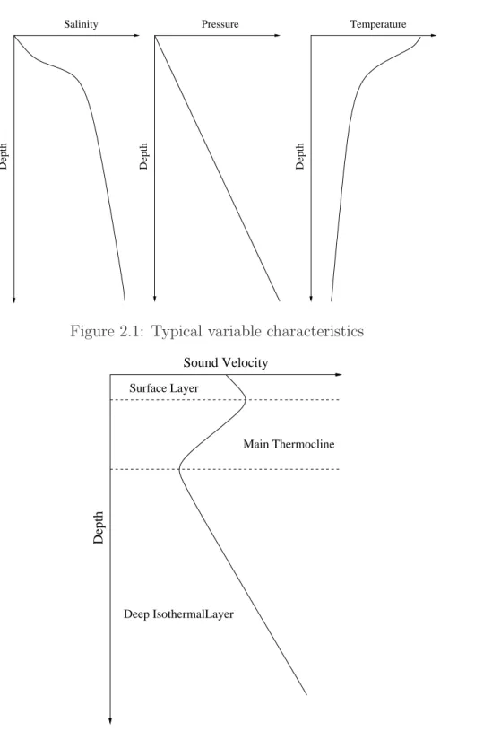
In underwater positioning problem, the medium (communication channel) is represented by sea water, thus the conventional aerial techniques of communications are not available. For instance light and magnetic signatures have limited communication range (< 100m) and radio frequencies do not propagate well in the water. Which kind of energy source should be used in an underwater positioning problem? An answer to this question can be found in Nature: sound energy. Sound under water is very important for animals: it allows them to navigate, to hear approaching predators and prey, and is a way of communicating with other members of the same species. The sound energy in the water, has a speed of propagation around five times greater than in the air. In a positioning problem, this characteristic is useful to cover long distance in a short period of time between the vehicle emitter and the receiver. The sound velocity is dependent upon various factors including water temperature, pressure and salinity. The influence of each variable is shown in figure 2.1.

Sea water is not an homogeneous body, it could be depicted as a stratified one where each layer summarizes the state of the three main variables (temperature, salinity and pressure). The sound path can be described as a ray by the Snell’s Law. The sound, when crossing a layer, deflects his path passing through the slowest propagation zone. The Speed Velocity Profile (SVP) is usually measured by a expendable bathythermograph probe, a typical SVP is shown in figure 2.2.

The SVP reveals some common structure to the ocean. The water can be divided into three vertical regions.The Surface layer is at the top and is the most variable part. As the name suggests, the profile will changes depending on the time of day and the season. The Main thermocline connects the surface layer with the uniformly cold water found deep in the ocean. Below about 500 m, all of the world’s oceans are at about 34◦_{F . The positive}

gradient in the deep isothermal region is solely due to the pressure effect.

In accord with temperature and sound velocity characteristic, three sea water conditions can be defined as follow:

• Isovelcity where sound propagation can be depicted as a long straight line, temperature decreases with depth and sound speed is constant (figure 2.3);

Salinity

Depth

Pressure Temperature

Depth Depth

Figure 2.1: Typical variable characteristics

Sound Velocity

Depth

Surface Layer

Deep IsothermalLayer

Main Thermocline

Figure 2.2: Typical sound velocity profile

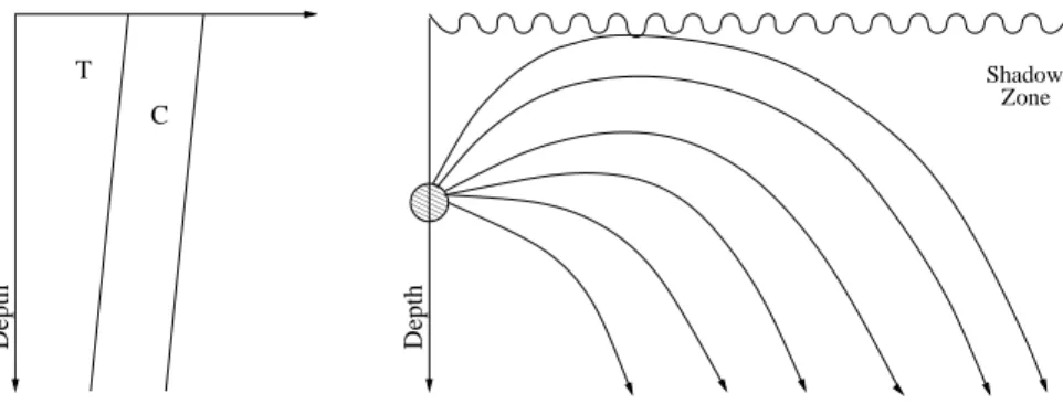
• Positive gradient where sound is bended in surface direction, thus the sound can not reach the seafloor. This effect is called Surface Duct. Postive gradient is characterized by warm water over cool water (figure 2.4);

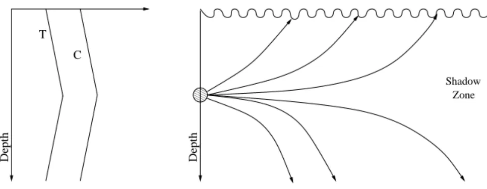
• Negative gradient where sound is bended in seafloor direction introducing shadow zones, in this condition, temperature and sound speed decrease with depth (figure

2.5). 00 00 00 00 11 11 11 11 Depth C P T Depth

Figure 2.3: Sound propagation in isovelocity water

00 00 00 00 11 11 11 11 Depth T Depth C Shadow Zone

Figure 2.4: Sound propagation in positive gradient water

00 00 00 00 11 11 11 11 Depth T Depth C Shadow Zone

Figure 2.5: Sound propagation in negative gradient water

In practical applications, the most common sea configuration is depicted by a first layer with positive gradient over a second layer with negative gradient. In this condition occurs the Layer Depth phenomenon defined as the depth where the sound velocity is maximum. Layer depth introduce a critical ray (sound propagation path) split, which creates a shadow zone as shown in figure 2.6, more sea water configuration are described on [29].

00 00 00 00 11 11 11 11 Depth T Depth C Zone Shadow

Figure 2.6: Layer Depth Phenomenon

2.2

Conventional Systems

Several commercial underwater acoustic positioning system are available. They are usually classified according to the concept of Baseline, which is defined as the distance between the active sensing elements. There are three common types, as define in [31]:

• Ultra Short or Super Short Baseline (USBL or SSBL) • Short Baseline (SBL)

• Long Baseline (LBL)

This dissertation is focused on AUV positioning problem, however the presented architectures can be also used for ROV, diver, and twofish tracking applications ([27],[31],[32]).

2.2.1

Ultra Short or Super Short Baseline

A complete USBL system consists of a transceiver rigidly mounted on the vessel bottom, and an emitter (Transponder or Responder) deployed on the underwater vehicle. Usually, the transceiver is composed by three or more transducers separated by a baseline of 10cm or less. A typical interrogation can be described as an acoustic pulse transmitted by the vessel transceiver, which is detected by the underwater vehicle sensing device, which replies with an acoustic pulse. The vessel transceiver catches the signal and it computes the range in accord with the elapsed time. A USBL system provides both the orientation and position between vessel transceiver and underwater vehicle emitter. Orientation is determined by a method called phase-differencing, which makes a phase comparison on arriving ping on vessel transceiver elements. Orientation and position determined by USBL are referred to the vessel reference frame thus the system needs a good accuracy level on vessel position.

Low system complexity makes USBL systems very convenient to use. Moreover, there is no need to deploy transponders on the seafloor. In order to obtain a good level of accuracy with an USBL systems based on Time of Flight (TOF) interrogation, the USBL sensing device need an precise instalaltion on the vessel, and a good absolute vessel position accuracy is needed, also.

Figure 2.7: Ultra Short Baseline

2.2.2

Short Baseline

A complete SBL system consists in a set of transceivers (≥ 3) rigidly mounted on the vessel bottom, and an emitter (Transponder or Responder) deployed on underwater vehicle. The transponders are separated by a baseline between 20 to 50 meters. The position determined with the SBL system is referred to the transceivers mounted on the ship hull.

Figure 2.8: Short Baseline

Low system complexity makes SBL system an easy tool to use moreover there is no need deploy transponders on seafloor, spatial redundancy and a good range accuracy with ToF system. In order to obtain that accuracy, SBL system needs large baselines in deep water (> 40m), detailed offshore calibration and a number of pole bigger than 3. As shown for USBL, AUV fixes are perform respect to vessel frame thus SBL require a very good vessel

positioning system.

2.2.3

Positioning Modes for USLB/SBL

In order to find a solution of AUV positioning problem USBL/SBL architectures offer two possible implementation:

• Transponder

• Free running pinger Transponder

Transponder mode relies on a bidirectional acoustic communication, the surface transceiver interrogates the vehicle device on a Interrogation Frequency (IF) and it waits for a response on a Replay Frequency (RF) from the vehicle emitter.

Free Running Pinger

A free running pinger (a beacon that constantly transmits at a known frequency with known repetition rate) is installed on the vehicle to be tracked, the depth information is given by a depth sensor. This approach is the least accurate mode for USBL/SBL architectures due to the inaccuracy of the estimate of depth, the clock drift, and sycronization errors. However this method provides the fastest update rate, which can have significant advantages when the positioning system is interfaced into a position control system, because the introduced delayes are smaller then the other positioning systems.

2.2.4

Long Baseline

Long Baseline systems are composed by three o more seafloor stations equipped with sensing device (Transponder or Responder), whose catch signals emitted by a transceiver mounted on the underwater vehicle. The position is determined using three o more time of flight ranges generated in the vehicle/stations communications. The fix generated is referred with respect to relative or absolute seafloor coordinates, thus a LBL system does not require a vessel positioning system. The seafloor stations are typically separated by a baseline between 100 to 6000 meters.

LBL system is capable of determing a position with a good of accuracy, independent of water depth and relative good accuracy for large areas. However the system complex-ity requires expert operators to deploy and recover the seafloor stations. Moreover, the deployment requires a comprehensive calibration and expensive equipments.

2.2.5

Positioning Modes for LBL

Conventional positioning modes for LBL architecture are: • Direct Ranging

• Intelligent Acoustic Remote • Relay

• Pseudo Ranging

Figure 2.9: Long Baseline and Direct Ranging

Direct Ranging

In direct ranging mode the vehicle transceiver interrogates the seafloor stations, it waits for the array replays and the on board processing derives a vehicle position. The interrogation process can be sequential or simultaneous. Sequential approach is based on a Individual Interrogation Frequency (IIF) and a Common Replay Frequency (CRF), insted simultaneous approach is based on a Common Interrogation Frequency (CIF) and a Individual Replay Frequency (IRF).

Intelligent Acoustic Remote

Intelligent acoustic remote mode is similar to direct ranging with simultaneous interrogation, but in this configuration, the initial time of interrogation is given by an acoustic command emitted from a surface control station. Also, the position is performed on surface control station, thus it is necessary a further communication between underwater vehicle and surface station. This solution is not reliable because the acoustic communication cycle plays a fun-damental role in the position update rate, which is slower then the direct ranging. About the fix accuracy, Direct Ranging and Intelligent Acoustic Remote have the same performances. Relay

Relay mode is a variant of previous one, in this solution the surface station interrogates the AUV transceiver on a Relay Interrogation Frequency, the vehicle device interrogates the

seafloor array by a CIF. The array replays and CIF are detected bye surface station, which knows his position respect to seafloor beacons thus it can perform the underwater vehicle position. Relay approach is more reliable than Intelligent Acoustic Remote, otherwise the fixes accuracy is afflicted by the inaccuracy of vertical range detection.

Pseudo Ranging

Pseudo Ranging is based on a synchronous communication between AUV transceiver and seafloor beacon. This solution needs a very low drift clock AUV pinger, which interrogates on CIF the array. The seafloor beacons replay on IRF’s, whose are kept by the surface control station which determines the underwater vehicle position. Fixes are estimated on time of transmission between the pinger interrogation and surface range detection. The drawback of this solution is the clock drift that introduces inaccuracy on fixes determinations, moreover vertical range detections introduce a further source of error. This implementation is rarely used.

2.3

Latest Architecture Developments

Starting from the architectures shown into previous sections, two are the main developments trends in acoustic positioning systems ([31]):

• System Integration • Inverting

2.3.1

System Integration

In system integration approach the conventional LBL/SBL/USBL are coupled with external sensors in order to improve fixes estimation accuracy. This solution is usually based in a Kalman Filter integration in fashion with aerial aided navigation. The advantage of this method concerns redundancy, more measurements are available in the system period, more sensor in the same operative area. Performance improvement are strictly relate with growing system complexity. Example of USBL/INS integration are described in [16].

2.3.2

Inverted architecture

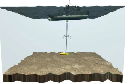
The inverting approach is based on inversion of the conventional acoustic system, most common inverted system are derived from USBL an LBL. In Inverted USBL approach the main advantage concerns signal noise ratio (SNR) in deep water, because in this configuration beacons are deployed on the seafloor close to the AUV operative area. Drawback of this configuration concern interelements coupling, for instance transducer and attitude sensor drift related to pressure, moreover power consumption when the system has to communicate with surface station. A brief introduction of this approach is given on [26].

Figure 2.10: USBL/INS integration scheme, from [16]

Figure 2.11: Inverted USBL, from [32]

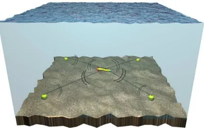
In Inverted LBL, seafloor stations are replaced by a surface beacons (usually buoys) equipped with a GPS system able to dertemine beacon positions. A free synchronized pinger (or a transponder) is installed on AUV, this device emit a pulse, which is kept from surface stations and it is transmit, by aerial communication, to main station to calculate AUV position. The estimate fixes are not transmit back to AUV, thus inverted LBL is limited to vehicle tracking. The commercial inverted LBL used in this thesis is ACSA/ORCA GPS Intelligent Buoy known as G.I.B., in next paragraph a detailed description is given.

2.4

G.I.B. System

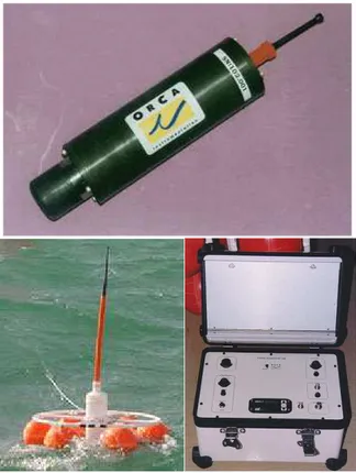
The G.I.B. (GPS Intelligent Buoy) system is composed by a set of 4 to 12 buoys equipped with GPS receivers and submerged hydrophones, an acoustic pinger with a frequency range from 8 to 50 kHz, and a control and display unit. The buoy network measures the Times of Flight (TOA) of acoustic signal emitted from the pinger to the buoys, at a known rate. The pinger is synchronized, prior to system deployment, with the GPS time.

During an estimation cycle, the pinger emits two consecutive pulses: the first is synchro-nized with GPS time and the second is delayed by an amount of time that is proportional

Figure 2.12: Inverted LBL, from [32]

Figure 2.13: GIB system

to the depth measured by a built-in pressure sensor. Each surface buoy transmits to the central unit the two measurements concerning the pulses emitted by pinger and their GPS positions.

The central unit converts the TOA in distances multiplying times by sound speed prop-agation in the water, which is assumed known (and constant). The acoustic source position can be then determined, resorting to trilateration or other estimation approaches. The main advantages of GIB system are relatively simple operation costs, no need to deploy or calibrate beacons on the sea bed, and independence of vehicle type.

Figure 2.14: GIB pinger (up), GIB buoy (left) and GIB central unit (right)