Nel capitolo 3 sono state riportate alcuni studi effettuati su un campione di dati storici relativi ai chilometri percorsi gli anni passati da tool dello stesso diametro e tecnologia. In questo allegato è riportata l’ultima analisi sviluppata per trovare qualche forma di stagionalità nei dati, che è stata effettuata da specialisti di statistica messi a disposizione dalla azienda. Come detto nel capitolo, questa volta sono state compiute più azioni sul campione, riportate nelle fasi successive.
Fase 1 - In primo luogo i dati sono stati analizzati graficandoli secondo una distribuzione normale, per definire chiaramente la loro appartenenza/non appartenenza a tale distribuzione.
Il risultato di questa prima fase è visualizzabile nel grafico 1.1. Grafico 1.1
Con i valori relativi riportati di seguito. Da sottolineare il grande valore della deviazione standard.
Descriptive Statistics: km
Variable N Mean Median StDev km 34 88,5 69,0 87,4
Come aspettato i dati si dispongono in maniera del tutto casuale, non seguendo quindi la curva della distribuzione Normale.
0 100 200 300 0 1 2 3 4 5 6 7 8 9 km F re q ue nc y
Fase 2 - Alla luce di questa affermazione, sono state applicate tecniche specifiche per dati non parametrici.
In particolare i dati sono stati testati con il Mood Median Test. In sostanza esso analizza i dati, suddivisi in categorie, per rispondere all’ipotesi
H0 - le mediane della popolazione sono uguali - contro l’ipotesi H1- le mediane non sono uguali -.
Una assunzione del Mood Median test è quella di considerare i dati di ogni popolazione come campioni casuali fra loro indipendenti, dove le distribuzioni delle popolazioni hanno la stessa forma. Questo test fornisce buoni risultati specialmente nelle prime fasi di analisi, ed è per questo che è stato scelto di applicarlo.
Il test è stato effettuato stratificando i dati secondo gli anni di appartenenza, 2003, 2004 e 2005 per verificare l’esistenza di un andamento generalmente simile nel corso del tempo.
Di seguito sono riportati i risultati del test effettuato sul campione stratificato per anni.
Mood Median Test: km versus anni
Mood median test for km
Chi-Square = 5,27 DF = 2 P = 0,072 Individual 95,0% CIs anni N<= N> Median Q3-Q1 ---+---+---+--- 2003 8 4 32 84 (--+---) 2004 7 5 32 113 (---+---) 2005 2 8 121 184 (---+---) ---+---+---+--- 70 140 210 Overall median = 69
Dai risultati ottenuti, si nota come l’ipotesi di mediane comuni debba essere scartata (sebbene due siano uguali) in funzione del valore di Chi – quadro (lontano dallo zero) e dal valore di P (probabilità) invece molto vicino allo zero. Inoltre è possibile notare come gli intervalli di confidenza (linee tratteggiate nello schema a destra dei dati) siano piuttosto grandi, quindi imprecisi.
Fase 3 – A riprova dei risultati ottenuti sono stati fatti ulteriori grafici e plottaggi dei dati, come il Box - Plot riportato nel grafico 1.2, dove è possibile notare lo scostamento che c’è tra i valori medi dei gruppi di dati (stratificati secondo i trimestri) e i valori massimi e minimi dello stesso periodo nei tre anni presi sotto esame.
Grafico 1.2
Il grafico deve essere interpretato con la seguente logica: più i box sono grandi (quindi, più si allontanano tra di loro la base inferiore e superiore del rettangolo) più il campione si dimostra irregolare; cioè, significa che i dati relativi allo stesso trimestre dell’anno, presi lungo i tre anni considerati, hanno valori tra loro molto diversi. Questo comporta che non è possibile basare le proprie previsioni considerando ciò che è accaduto nello stesso momento dell’anno gli anni passati.
Infine si riporta un ultimo grafico (grafico 1.3) nel quale è possibile notare le disposizioni dei valori massimo minimo e medio per ogni quadrimestre e l’anno di appartenenza di ogni valore.
1 2 3 4 0 100 200 300 quadrimestri km
Grafico 1.3
Dal grafico si nota che i valori massimi siano relativi al 2005 (ad eccezione del 4° quadrimestre, ma è da ricordare che i dati del 1005 arrivano fino ad ottobre), metre i minimi e i medi si alternano tra 2004 e 2003. Il fatto di avere i valori massimi del 2005 è comprensibile considerando il trend crescente che è stato trovato. L’alternanza degli anni 2004 e 2003 nei valori medi invece va a consolidare quanto finora affermato: cioè che non è possibile fare analisi statistiche basate sugli anni passati. Infatti, a rigor di logica, si tenderebbe a pensare che se i valori massimi sono imputabili al 2005 a causa del trend crescente, quelli medi spetterebbero al 2004, regola che invece non è sempre rispettata.
ALLEGATO 2
Procedure for the “EVALUATION MODEL”
SCOPE:This procedure is to create a file that will give an estimation of the spares volume for the future according to what has happened in the past.
The historical data used by the model are the issue and return transactions item quantity, usage and the costs of issue and return.
The estimation is based on the planned kilometers for the future runs. The file created will be a three levels:
1. The fist level is the total quantity for kms, total issue, total return and total cost divided by sizes of tools. That gives an estimation of the total of transactions and cost of a year, or in general, for the period that want to be considerate according to the forecast of run in MST.
2. The product of the pipelines characterizes the second level. The products are splat in 4 categories: “gas”, “oil”, “water” and “other”. In this sheet it’s possible to have issue, return ad costs size-by-size and product-by-product.
3. In the last level the issue, return and costs will be splat in On BOM items and Not On BOM items, in order to underline the differences between these two spare types. As in the other, also in this sheet it’s possible to have an evaluation of the future quantity just introducing the planned kilometres sorted by size and product.
All of the sheets have got links size by size to the items list sorted by issue, return and the calculated usage. Plus to that for each items will be reported an evaluation of the future quantity.
INDEX
- 1. DATA recruitment………..………...…124
1.1Data needed………124
1.2How to get the data………124
- 2. DATA elaboration………..133
- 3.Creation of the EVALUATION MODEL file………143
3.1Product sheet ……….143
3.2 Total Quantity sheet………..148
3.3 On BOM & not on BOM sheet……….152
3.4 How to use the file……….154
- APPENDIX 1 ……….155
Part 1- Excel pivot table ……….155
Part 2- Excel actions………160
Filter………160
Sort……….160
Hyperlink………161
Useful Advice………163
1. DATA recruitment
1.1 DATA needed- Global year usage of the last year (2005) GYU - Master Scheduler Tracker file of 2006
- Runs of last years (2005) (taken from Master Scheduler Tracker-MST)
- Unique list of the spares kit items BOM.
- BOM for all the items (on BOM- i.e. spares for option kit, and not on BOM spares): those can be found with the GTs.
1.2 How to get the data
Global year usage: it is a report of the Inventory transaction of the last year.
You can find it in Oracle discoverer.
Master Scheduler Tracker: it is located in e-Delivery. Log on in e-Delivery
and click on the Award view (view only), then click on Master Scheduler
Tracker (view only) (Figure I).
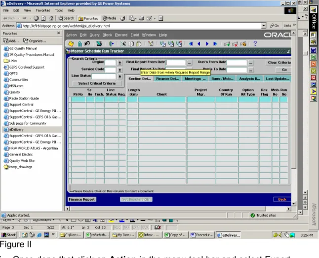
a. Open the Master Scheduler Tracker (view only) and click on the Final report from date space and introduce the data from which you want the future forecast. Now click on Final Report
To date and insert the data till when you want the forecast
(Figure II). Figure II
b. Once done that click on Action in the menu tool bar and select Export. That will create an excel sheet with all the data of the MST.
c. Save the excel sheet on your computer, naming it as “MST 2006”.
d. Close the web page and open the “MST 2006” file created. e. Go to the tool bar and click on Tool and select Filter.
f. Now click on the little arrow that have been created in the column of Technology, and select the tool technologies of your business. Now click on the arrow in the column Preparation Tool country and select your country.
g. Copy the entire sheet in a new worksheet: this is your future forecasted plan.
Last years ran: basically they can be taken from the MST of the last year.
- However the Black Belt- quality team should have it or be able to run a report. (In that case the report have to have: -number of project, technologies of tool, tool size, kilometers for each project, country of inspection, product of the pipelines inspected).
Option Kit BOM: you should find the BOM in the company database.
If there isn’t anything, follow the next instructions.
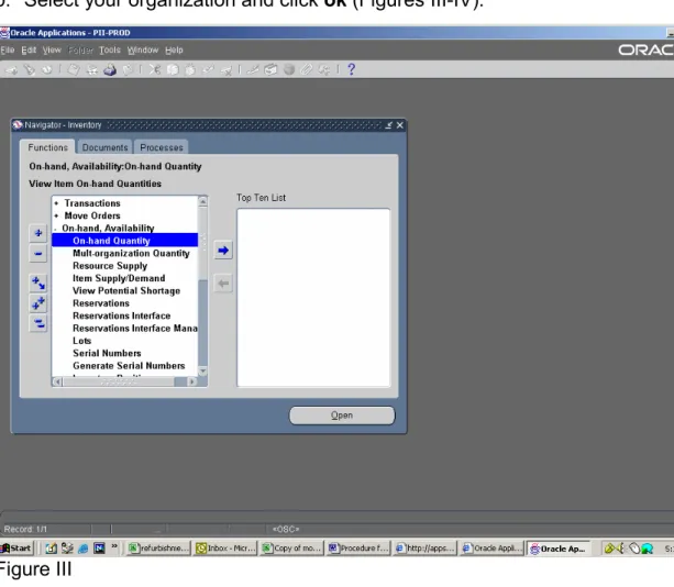
a. Log on in Oracle, dominium Inventory, click on On hand
Availability, and then on On hand Quantity.
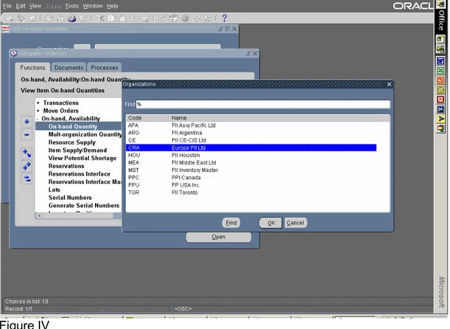
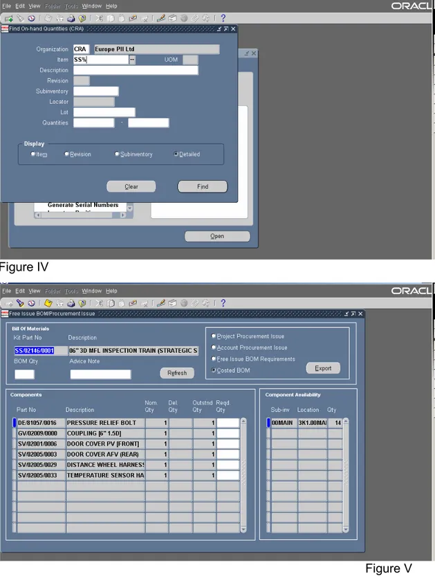
b. Select your organization and click ok (Figures III-IV).
Figure IV
c. Now in the new window write the first two digits of your BOM followed by % symbol (i.e. SS%) in the Item space and click on Detailed and then click on Find (Figure V). Figure V
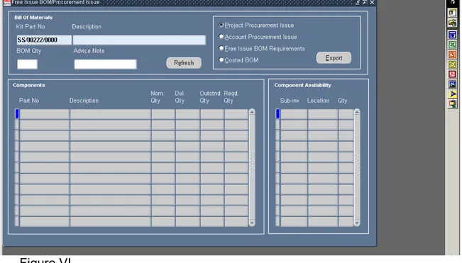
d. After that press Ctrl and F11 digits on the computer board. Should appear a new screen as shows figure VI.
Figure VI
.
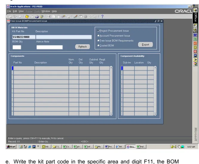
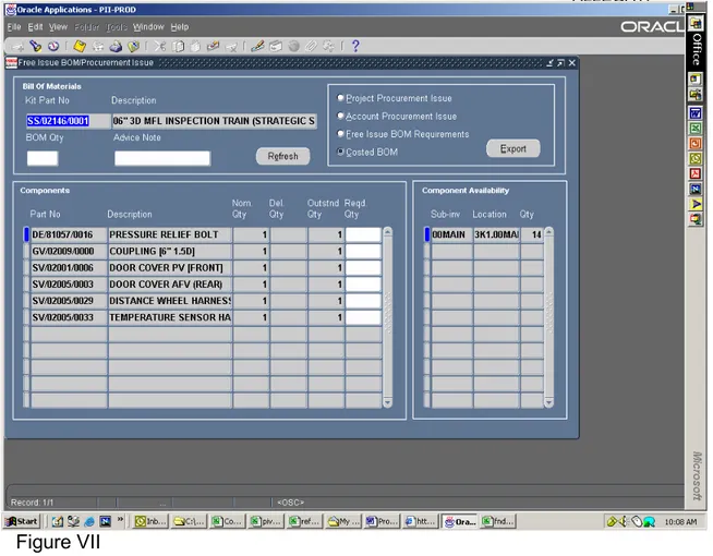
e. Write the kit part code in the specific area and digit F11, the BOM should appear (Figure VII).
f. Click on Costed BOM and then on Export (Figure VII). An excel sheet should been opened thank to that action. Save the file on your computer naming that as the tools size it belongs
g. Repeat the actions from step k to j. An advice is to put all the BOM of the same tool size in a unique sheet. Figure VII
h. Take all the files created and put the data together in a unique excel sheet. In this way you will have a unique list of all the BOM, for all the ON BOM item.
Figure VII
GT BOM: if you don’t have the GT BOM already as an excel list in your data
base, follow the next actions: a. Get the GT part codes list.
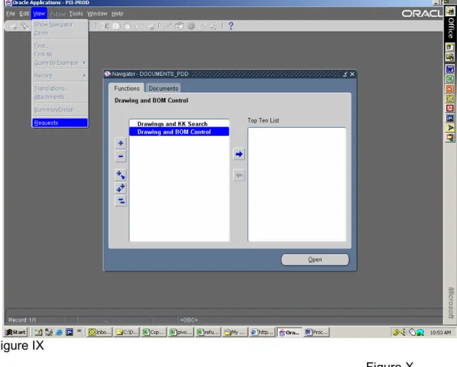
b. Log on in Oracle and choose the DOCUMENT_PDD responsibility. Select Drawing and BOM control and click on View on the tool bar. Then click on Request. (see figure IX)
c. After that a new screen should appear. Click on Submit a new
Request, and then, in the new little windows that will be opened click
on Request set and then OK. (Figure X)
d. In the new screen that will appear click on the icon (…) of Request set. After that a new window, called Sets will be opened.
e. Click on PII Drawing Folder Request set and OK. A new screen should appear.
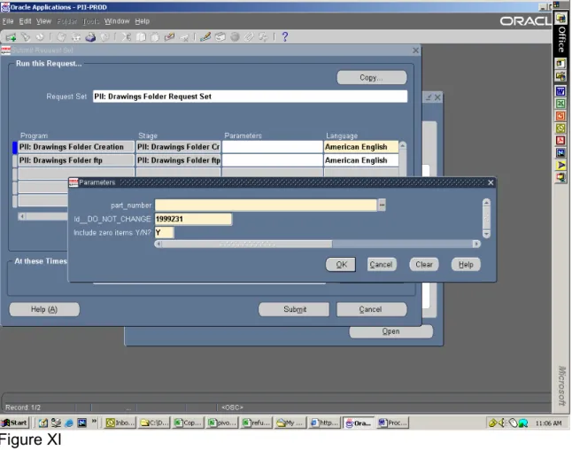
f. Click on the space below Parameters. A new little window should appear (See figure XI).
Figure IX
Figure X
g. Introduce a GT part code in the space part_code and click OK.
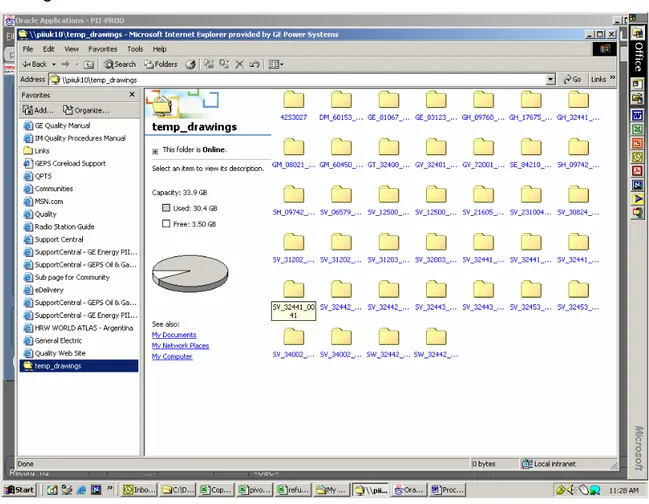
you can find the folders of the GT part code that you have request, and inside that there will be its BOM (probably you’ll have to wait some minutes before the GT folder appears).
Figure XI
i. When the GT folder has come open it. Inside the folder there will be several Drawing files, but only one will be an excel file. Take that one and save it on your computer, keeping attention to save it as an excel file (extension: .xls). An advice is to save it as the size tool it belongs.
Figure XII
j. Repeat steps from g till i until you haven’t extract all your GT part codes.
2. DATA elaboration
1. Take all the GT files created before.
2. For each size of tools make the following actions:
a. Take one by one the GT BOMs and make a pivot table taking the “Part code” and the “Quantity on tool”. (That is needed to be sure that there will be not duplications of the same item in the same BOM. Be aware to set on SUM for the calculation of Quantity on tool). If you don’t know how to do a pivot table see appendix 1- part 1)
b. Add a column, next to the pivot table, writing the size of the tool, as shows figure 1.
Figure 1
3. Create a unique file putting together (one below the previous) all the data of the pivot tables. It has to be a list of item not in the pivot tables. A way to do that list is to copy the items from their pivot table and paste them in a new worksheet. (If you want to copy only the part item list of a pivot, but don’t want that the pivot would be still active, the only way is to start to select the cells that have to been
copied from a cell outside the pivot and don’t take the buttons in the top of the pivot). The final list should be a continue list where are presents all the GT BOM for all the items, and their tools size.
4. Make a pivot table of the list made in the step 3. In that pivot should be put the “Part code” in the first column (as rows of the table) and in the body part the “size” and the “Quantity on tool”. The output should be a table where for each item it is possible to see all the sizes where it is assembled and the quantity, as shown in figure 2 (see APPENDIX 1- part 2).
Figure 2
5. Take the option kit spares BOM file and add a column writing “On BOM”, it will be a entire column with the same contents for all the items of the list.
6. Take the Global Year Usage of last year (GYU), add a column and make a VLOOKUP the with the “spares option kit BOM” selecting the column made in the previous step (the “ON BOM” column). That action is useful to identify which items of the GYU are spares part for the option kit, and whose are the “not on BOM items”. Go to
7. Take the last year file of Global year usage and add as many columns as many are your tools sizes. Write in each of them one size of the tools as title (i.e. the first column will be titled as the same size that you have put in the pivot table made in step 4). In other words at the end you’ll have all your tools size as titles, as you can see in figure 3).
8. Click on the first cell below the title (size) and do a VLOOKUP with the made pivot table (of step 4), selecting the column number refers to the same size and extend the VLOOKUP for all the items listed in the Global Year Usage. Do the same actions for all the other tools size you have put as titles in the step 7. The output should be a file that shows for each items of GYU on whose tools they can be assembled (an example is reported in Figure 3). (If the file dimension is too big, it is possible to divide the Global Year usage in two different files: Issue and Return. To make the issue it is necessary to take all the transaction called: “Project Issue”, “Miscellaneus Issue” and “Intransit shipment”, copy them and paste in a new excel worksheet. To make the Return file it is necessary to take all the transaction called: “Project Return”. “Miscellaneus Return”, “Intransit return”, copy them and paste in a new excel worksheet. 9. Take the Runs of last year (MST of 2005) and filter the data in terms
of the size (one size per time) and the region of analysis (it has to be the same of the region of the one of the GYU).
Figure 3
10. Take note of number of projects, kilometers ran and product of
the pipes inspected for each size of the tools. To make faster the
following steps it’s suggested to sort the number of projects by the product.It could be useful to use tables like the one presented below.
11. Do this action for all the size of the tools. 12. Take the GYU and
filter the data by the
tool size, the
number of project
and the transaction (has to be ISSUE). In other words, filter by the size of tool (i.e. start with the first of your list), filter the file by the numbers of project made for that tool size and filter on the transaction, taking the Issue.
Size of tool Num of project Km ran Product 100000 23 GAS 100100 57 GAS 20010 15 OIL
13. For each number of project that you have filtered (for the same size of tool) copy the data and paste it in a new worksheet created where have to be put all the data of the same size. It necessary to create new sheets for each product of pipes inspected by that tool size. Figure 4
14. Make also a sheet with all the projects data together.
15. Repeat steps 11, 12 and 13 but this time filter the transaction as
Return. As output the sheets created will be as many as the products
inspected plus the total of issue and the total of return. In the figure 4 there is an example.
16. Take one by one all the files done, and create pivot tables for each worksheet created in the previous steps. Select the area from “part code” to the column “on BOM/not on BOM”. The pivots should contain part code and the On BOM/Not on BOM in the first column and the transaction quantity in the body part.
There are as many sheets as the many are the product of inspection (in this case OIL and GAS) plus the total, for the issue and then for the return.
17. Put in different columns the pivots for the issue items and the pivot of return items of the same product, as represented in figure 5. It is suggested to put all the pivot tables in the same sheet, in order to have all the products summaries in the same page, name that sheet as “PIVOT TABLES”.
Figure 5
18. Now it’s necessary to calculate the difference between the transaction quantity of the issue and the return, in order to find the real usage quantity. The quantities of the two transaction types have to be represented in different math signs (i.e. issue transaction quantities are with the “-“ sign, while the return transaction quantities are with the “+” sign). To achieve the usage quantities it’s possible to follow the next actions:
a. Take the data inside the pivots table for the issue and the return of the same product and tool size (with the copy action) and put them in the same columns of a new worksheet (for example issue data above return data).
b. Create a pivot table of that new list (issue/return). The pivot will be with part code in the first column (as rows) and quantity in the body part, and as usual the summarizing formula has to be the sum.
c. Once you have done the pivot take only the negative values from that (or in general the value with the same sign of the issue transactions), those items are the used items.
d. Take the list of the used items and copy that in the sheet where is the original pivot tables, as showed in figure 6.
Figure 6
19. To have the items description a select a cell in the same row where there is the first item of a pivot list and make VLOOKUP with a file that has got the same part codes (or even more) of the pivot table and the description of the items.
20. Repeat the previous steps for all the products of all the size tools and for the total quantities.
21. It is useful also put in evidence which items are more requested than the others. In other words, underline which items are requested in
most of the projects. It’s possible to obtain that working on the TOTAL pivot tables done, following the next step:
a. Copy the total pivot table of one specific tool size in another new excel worksheet (you can open a new book).
b. Drop the Transaction quantity in the pivot window, in order to empty the table (should stay only the bottom of Part code).
Figure 6a
c. Now drop the project and the transaction quantity in the space for the column field as shows figure 6a. (an example of this steps is reported in APPENDIX 1–part 2).
d. Drop the transaction quantity in the body part. Set the type of summarizing on Count.
e. You should see a table that has got as rows the items and as columns the projects number, and as body part the count of transactions. (See figure 6b).
Figure 6b.
f. Now you should count the number of time that the same item is present for the different project. An easy way to do that is to write the following formula: “=COUNT(B2:I2)” in a cell out of the pivot table aligned with the part item list and (where B2 and I2 are example but have to be the first and the last cells of the body for the same row).
g. Now, to make the classification of the more requested items it is necessary to take the items that are at least counted for more than the half of the projects quantity.
h. Open the sheet with al the pivot tables and report the top items (i.e. one in the right side of the sheet).
i. You can add the description of the items (you can do that making a VLOOKUP with the ISSUE sheet). The file should appear as shown in figure 6c.
Figure 6c
22. Put all the files created in the same folder. 23. The files are created.
3. Creation of the EVALUATION MODEL file
3.1 PRODUCT sheet1. Take the sheets created in the “data elaboration” and take note of the total quantity and cost of issue and return items for each product and each size.
2. Take the table created in the step 10 of “Data elaborations”.
3. Create a new Excel worksheet and write the data taken previously (for each tool: product of inspected pipe, ran kms, issue quantity, return quantity, cost issue, cost return), creating a list with the information of all the tool sizes, as showed in figure 7. That data will be the part of historic data (2005) used by the model. Name the sheet
as “Product”. Figure 7
5. Because the MST defines the runs planned as “Awarded –plan”, that are run with a very high probability to be run, and “Award – no plan” and “Prospect”, that are not very sure to be run, calculate the 100% of “awarded- plan” and only the 50% of the other two definitions. It can be useful add a column in the MST and insert the formula: “=IF(D2=“Awarded-Plan”,D2,D2/2)”. (D2 here is just an example, but it has to be the cell with the km of the run). Otherwise, consider of the km “awarded –plan” and separately the kms of “awarded-no plan” and “prospect”.
6. Take notes of the all forecasted kilometers of run (filtered by size and product).
Figure 8
7. Take the file “Product” and add a column inserting the kms taken from MST. Those data will be in a new section called “forecast”, where will be put the evaluation of all the values. If in the step 5 has been calculated the formula (“=IF(D2=“Awarded-Plan”,D2,D2/2)”) then report directly in one column the total kms. If the formula hasn’t
“awarded- plan” and one for the others. In this case it is also necessary to create a 3rd column where has to be put the formula to take only the half of “awarded - no plan” and the “prospect”. The formula can be “=(I5+H5/2)” (where I5 and H5 are example, but have to be respectively the cell of “Awarded-plan” kilometres, and the cell of “awarded – no plan” and “product” kilometres).
8. Now it is possible to do the evaluation of the future quantity. Add columns next to the 2006 kms for the “forecasted issue”, “forecasted return”, for. Cost issue” and “for. Cost return”.
9. To make the evaluations of the quantity based on kilometers has to be write an equation for each the categories we want to forecast. The basic equation is:
a. “quantity in 2005 : km of 2005 = quantity in 2006 : km of 2006”. Our unknown quantity is the “quantity in 2006” that will be found with:
b. “quantity in 2006 = (quantity in 2005*km of 2006 )/(km of 2005)”.
c. So in the column of “for. Issue quantity” has to be put the formula: “=(D7*J7/C7)”, where D7 is an example but has to be the cell of 2005 issue quantity, J7 has to be the forecasted kilometers of 2006 (with 100% of “awarded –plan” and 50% of “awarded- no plan” and “prospect”) and C7 has to be the Kilometers cell of 2005.
10. Put the formula presented in step 9 for each forecast quantities (return, cost issue and cost return) and be aware to change the quantity of 2005. For the forecasted return the “2005 quantity” has to be the “2005 return”, for the “for. Cost issue” the “2005 cost issue” and for the “for. Cost return” the “2005 cost return”.
Figure 9
11. Do actions of step 10 for all the product of the same size and for all the size, achieving a sheet as showed in figure 9.
12. Now add as many sheets as the tool sizes quantity in the EVALUATION FILE.
13. Get the files created in the Elaboration Data and for each one copy its the “pivot tables” sheet in a new sheet created in the EVALUATION MODEL file, naming the new sheet as the tool size you have entered. In this way you will have all the pivot tables of the tools in the same file.
14. Now go in the “product” sheet of EVALUATION MODEL file and click on a cell that “belong” to the area of one size and create a hyperlink (right of the mouse, choose “hyperlink”. See APPENDIX 1- part 2) with the new sheets created. For each tool size has to be made a hyperlink with its sheet previously created.
3.2 TOTAL QUANTITY Sheet
1. Create a new sheet named “total quantity”.
2. From the “product“ sheet take the total of “issue 2005”, “return 2005”, “cost issue 2005” and “cost return 2005” of each size.
3. Create a table as showed in figure 11. To avoid you to fill the table in with the data, it is better to create link with the “product” sheet. You have just to select the row below KM and put the sign “=”, then come back to the product sheet and click on the row corresponding to the
total kilometers of the same tool size you are filling in. If you have
done it properly you should see in the cell where you are working the total of KM ran for that size (the same that is written in the other sheet).
4. Do the same action for all the other data (issue, return, cost issue and cost return, and also the total kilometers for the 2006/future, taking the cell with the total km). That will allow you to insert the data only in the fist sheet when you will use the file. The output is showed in figure 12.
Figure 12
5. Now it is possible to do the evaluation of values using the same equation mentioned in step 9 of “PRODUCT” sheet. So to forecast the 2006 “issue”, write the formula “=(D5*J5/C5)”, where D5 is an example but has to be the cell of 2005 issue quantity, J5 as to be the kilometers of 2006 forecasted (with 100% of “awarded –plan” and 50% of “awarded- no plan” and “prospect”) and C5 has to be the cell of 2005 Kilometers.
6. Put the formula presented in step 5 for each forecasting quantities (return, cost issue and cost return) and be aware to change the quantity of 2005. For the forecasted return, the “2005 quantity” has to be the “2005 return”, for the “for. Cost issue”, the “2005 cost issue” and for the “for. Cost return” the “2005 cost return”. (To have entire
values has of issue and return It can be used the function ROUND. So the final formula of the forecasted issue cell would be: “=ROUND(D5*J5/(C5),0.5)”).
7. Do that for all the product of the same size and for all the size, achieving a sheet as showed in figure 13.
Figure 13
8. Click on a cell that in the same row of a specific size and create a hyperlink (right click of the mouse, choose “hyperlink”, see APPENDIX 1- part 2) with the final sheets whit the tools pivot tables. For each tool size has to be made a hyperlink with its file previously created.
9. To have a direct evaluation for the issue and return values item per item follow the next instructions:
a. Click on the link created and open the “total pivot” sheet. b. Write in a cell the km of 2005 ran for that tool size.
c. In the cell below write the tool size (it has to be written perfectly the same as in the “total quantity” sheet, otherwise the following actions
d. Next to that cell create a VLOOKUP with the “total quantity” sheet, selecting as Lookup_value the cell with the size, as Table_Array put the “Total quantity” sheet and as Col_index_num put the number of the column where there are the Kms of 2006. The function will give as output the km of 2006 of the size selected in that cell. e. Add a column next to the quantities of the issue pivot and put the
formula “=ROUND(B7*$G$2/$G$1,0.5)”, where all the letters and number are examples but has to be: B7 represents the issue quantity of an item, G2 represents the cell where is the 2006 km and G1 represents the cell where is the 2005 km.
f. Extend the formula for all the issue items and also for the return and the usage. The output is showed in figure 14.
Figure 14
3.3 on BOM & NOT on BOM sheet.
1. Take the files created in the “DATA elaborations” section.
2. For all the issues sheets (for the different products) take notes of the on BOM “issue items”, “Usage” total quantities and “cost”. Do that also for the Not on BOM (to do it quicker sort the sheets by the “On BOM” column. See APPENDIX 1-part 2 for the Sort actions).
3. Do the action of step 2 also for all the returns (taking quantities of return transactions and the cost sorted by on BOM).
4. Create a new sheet in the “EVALUATION MODEL” file, naming it as “on BOM & not on BOM”.
5. Write all the taken data in the previous steps as showed in figure 15.
Figure 15
6. Add a row for each size inserting the total of the quantities written (i.e. total of issue, total of return on BOM and not on BOM). The formula that has to be written in each cells is simply the sum of the cells for the same categories, “=SUM(C5:C8)”, where C5 and C8 are examples, but have to be C5 the “GAS” quantity ,and C8 the
7. Add a column with the ran kilometers of 2005, divided by products and sizes.
8. Now add a column where insert the future km planned. Create a link with the sheet “product” to obtain the data already written in that sheet. To do the link insert the “=” symbol in the cell below the KM title and go to the “product” sheet selecting the cell that has got the total km for the same product and size where you are working on. If the link has been done properly you should see the km that are also in the product sheet. Do that for all the product of oll the size.
Figure 16
9. Now repeat the steps from 7 to 9 of the “total quantity” sheet. This time the data are divided on “on BOM” and “not on BOM”, so, be aware in choosing the right cells while you are writing the equation formula for the evaluation. The output of this action it is showed in figure 17.
10. Finally, add two columns where put the calculation of the percentage of used quantity on the issue quantity, on BOM in one column and not on BOM in the other. The equation is: %=(usage quantity*100/issue quantity) and have to be values of 2005.
Figure 17
11. The “on BOM & not on BOM” sheet is completed.
3.4 How to use the file
Once the file is completed, to use it and have the evaluation it is necessary to insert the forecasted kilometers of 2006 in the sheet “Product”, and the file will calculate all the values.
APPENDIX 1
Part 1- Excel Pivot table
The pivot table is useful when you’ve got a list with duplications or you want to underline some aspects of that. The pivot will give as output a list where the items composing are reported just once. The pivot it is also useful because it is possible to obtain some calculation as the sum, or the count of the data.
To create a pivot table you must have a list of data that at least has got two columns (of course the file has to be an excel one!). The list has to have titles for each column and there have no to be white rows at the top: in other words the titles will be put in the row number 1.
1. Go to the tool bar and click on Data, then click on Pivot Table and
Pivot Chart Report, a window should appear.
2. Following the wizard click on Next button.
3. The new window asks you to put the range: you have to select the columns you want make the pivot table.
4. Then click on next and follow the wizard. You can choose if put the pivot table in a new worksheet or put in a existing sheet. If you want to do the first just click on Next, if you want to put the pivot table in an existing sheet, then you have to click on Existing worksheet and put in the space the columns you want to put the pivot table.
5. Then click finish. The pivot table skeleton should appear in the new worksheet or in the column you choose and should be also a pivot table window where are written all the titles of the columns you took to make the pivot (see figure 2).
Figure 2
6. Drop in the first column the title you of the column you want as first of list and that will became the rows of the table (in the procedure has always to be the column with the items Part code). See figure 3.
Figure 3
7. Drop the column title you want to summarize in the place where it’s written “Drop Columns Fields Here”. In the procedure the data that are in general been put here are the Quantity on tool (or the Transaction quantity). After that, drop the new button created in the place where it is written “Drop Data Items Here”
8. As result of that action the list should appear as showed in figure 4. 9. Now you can choose which summarizing type a you want to be done
on the data that you dropped down.
10. Should be already one summarizing type as default (the type is written in the first cell of the first column). If you want to change it click on Pivot table of the tool bar of the little pivot window and select
Field setting. Another little window will be open and here you can
choose the type of summarizing. For the procedure mostly it is requested the Sum type (see figure 4).
Figure 4
Part 2- PIVOT TABLE requested in step 4 of DATA Evaluation section
- Follow the instruction from step 1 to 6 of APPENDIX 1-part 1, putting as first column of the pivot the Part code.
- Drop in the place where it’s written “Drop Columns Fields Here” the
Quantity on Tool and the Size (one per time), as shows figure 5.
- Drop the “Quantity on tool” button in the space where it is written
Drop Data items here.
- Then select the Sum in the summarizing type, as descript in step 10 of APPENDIX 1 – part 1. The pivot should appear as figure 6.
Figure 5
Part 2- Excel Actions
Filter
Very often in the procedure it is useful to filter the data. It is very easy to do that. You can follow the next steps:
1. Click on the row you with the titles of the list. 2. Go to the menu tool bar and select DATA. 3. Click on Filter and then click on Autofilter.
4. After that on all the cells selected should appear a little arrow. If you click on the arrow a window should be opened, showing all the voices that are content in that column.
5. Now if you click on one voice of the list that will shows you only the items that are characterized by the voice you choose.
Sort
Another action that can be useful is the Sort. Its objective is to sort the list by an order you choose and by a column you decide. To obtain a sorted list follow the next steps:
1. Select the list you want to sort (it is important to take all of its columns otherwise the sort will be done only in the selected columns and not on the non selected ones, that means that the data of the non selected columns will not be sorted as the others and so the relations won’t be right.)
2. Go to the menu toolbar and click on DATA, then click on sort.
3. Choose the order you want to sort the data and choose the column you want to sort. (See figure 7)
Figure 7
Hyperlink
The hyperlink allows you to relate together different file or different sheets in the same file. In fact clicking on a “link” you can open directly a different file or a different sheet. To do the hyperlink between follow the next actions:
a. Select a cell on your excel worksheet.
b. Right click of the mouse, a window will be opened. You can find the Hyperlink voice at the bottom of that window.
c. Clicking on Hyperlink a new window will be opened. Here you have to insert the file name you want to create the link between. You can write it directly in the proper space, or click on Browse for and File and search your file. See figure 8.
d. If you want to make the hyperlink between different sheet belonging to the same file do the action from step a to step c, but this time in the part Link to: you have to select Place in this document. Doing that you can select the sheet you want to make the link with in the list that will be showed. See figure 9.
Figure 8.
e. Once you have choose the file you can write the text you want will be displayed in the cell you are working on.
f. Then click on OK, the Hyperlink should have been done. You should see the text you have written on the cell selected in a different color (blue) and underlined. If you click on it the linked file should be opened. g. If you want to make the hyperlink between different sheet belonging to
the same file do the action from step a to step c, but this time in the part Link to: you have to select Place in this document. Doing that you can select the sheet you want to make the link with in the list that will be showed.
Figure 9
Useful Advice:
In excel the symbol $ it is used in the formulas to have fixed columns or rows. For instance: if you put in a formula the value $C$1 and drag the same formula for more cells, the value of the cell C1 will be consider for all the cells, and not only the first one.
You can use $ also to let fixed only cells or rows by themselves, like $C1 or C$1.
APPENDIX 2
VLOOKUP function.Excel has got several functions useful to get some calculations and to relate together data.
The more used in the procedure is the VLOOKUP function. It means Vertical look up, and its function is to search a value in the leftmost column of a table and to return a value in the same row from a column you specify. In other words, you should have two different tables where there are some cells with the same values. The values that you put as Lookup_Value will be searched in the other table (that you will put in the Table_Array) and as output you’ll have the value that is in the same row of the founded value looked up, but belonging to a column you choose.
Lookup_Value : is the value to be found in the fist column of the table, and
can be: value, reference or string .
Table_Array: is a table of numbers, text or logical values in which data is
retrieved.
Below there is the explanation how to make that.
Col_index_num: is the column of the table array from which the matching
value should be returning.
Range _loop: is a logical value (true or false): to find the closest match in
the first column (sorted in ascending order), and has to be FALSE for the procedure issue.
To do a VLOOKUP follow the next steps:
1. To enable the functions it is necessary to write in a cell the sign ”=”. 2. Doing that the functions button on the left side of the sheet should
3. Selecting VLOOKUP a new window will be opened.
Figure 1
4. Click in the Lookup_value space and insert the column you want the value will match its values. Figure 2
Figure 3
5. Click in the table array space and go to the table you want to retrieve the matched values.
6. Click on Col_index_num and insert the table array column number that has the values you want to be returned.
7. Finally, in the Range_loop space insert FALSE.
8. The VLOOKUP has been done. If it has been done properly you should see in the cell where you have worked the value you were looking for.
9. If you have a list that you want to find the VLOOKUP, you can extend the same formula written in the first cell just clicking on that and dragging down the arrow.
10. In the figure 3 there is an example where you can see the VLOOKUP window filled in. The underlined column is the one where the VLOOKUP has been reported. The table array is a different file (that should be open before select the VLOOKUP function), and the values wanted be returned are in the second table array column.
ALLEGATO 3
Procedure for “ORDER QUANTITY MODEL”
SCOPE & OBJECTIVESTo give the Inventory a guideline of the item quantities to buy according to the kilometers planned for the next future and the min max model.
The model is for all the items that create a tool and specifically there is a calculation for the refurbishment according to kilometers and inspection regions.
The model is divided in three group of sheets:
1. The template: the interface where have to be put the external data that will be used in the model. This sheet will give also the quantity to be ordered. There is a second sheet where have to be put the planned kilometers for the next future for all the tool sizes.
2. The Refurbishments file: where are all the types of refurbishment. Form the standard spares till the 5th refurbishment. This file is linked with the kilometers planned in order to define the quantity of each refurbishment needed.
3. The GT BOM: a pivot table where are all the items of the tools.
The action that are request to use the model are to update some of the information inside the model, as the on hand quantity, the PO work in progress and to put the future run kilometers and the country of inspection which the items quantity is needed. All the other data will be updated by themselves.
INDEX
1. Data needed….……….……….169 1.1 How to get the data……….169 2. Creation of “Order Quantity Model” file………..177 2.1 “Kms planned” sheet……….177 2.2 Creation of “Refurbishment file”…… ……….182 2.3 Creation of “Quantity on tool“ file………186 2.4 Creation of the “Template” sheet in ORDER MODEL file……..189 2.5 How to use the model………...191 APPENDIX 1………..192
Part 1- excel pivot table………..………192 Part 2- excel actions………196 APPENDIX 2- VLOOKUP function……….197
1
. DATA needed:
- Master Scheduler Tracker file of 2006 or similar model that tells km of run and country of inspection.
- BOM for all the items (on BOM- i.e. spares for option kit, and not on BOM spares): those can be found with the GTs.
- Refurbishments BOM and quantities.
- Kilometers triggers to define the different refurbishments needed. (i.e. until 80 kms -> standard spares, from 801 to 160 -> 1 ref, and so on) - Stock On hand quantity.
- PO work-in-progress. - Min max values - Items classification.
1.1 How to get the data
:
Master Scheduler Tracker: it is located in e-Delivery. Log on in e-Delivery
and click on the Award view (view only), then click on Master Scheduler
Tracker (view only) (Figure I).
h. Open the Master Scheduler Tracker (view only) and click on the
Final report from date space and introduce the data from which you
want the future forecast. Now click on Final Report To date and insert the data till when you want the forecast (Figure II).
Figure II
i. Once done that click on Action in the menu tool bar and select Export. That will create an excel sheet with all the data of the MST.
j. Save the excel sheet on your computer, naming it as “MST 2006”. k. Close the web page and open the “MST 2006” file created.
l. Go to the tool bar and click on Tool and select Filter.
m. Now click on the little arrow that have been created in the column of Technology, and select the tool technologies of your business. Now click on the arrow in the column Preparation Tool country and select your country.
n. Copy the entire sheet in a new worksheet: this is your future forecasted plan.
Option Kit BOM- refurbishments: you should find the BOM in the
company database.
If there isn’t anything, follow the next instructions.
a. Log on in Oracle, dominium Inventory, click on On hand Availability, and then on On hand Quantity.
b. Select your organization and click ok (Figure III). Figure III
c. Now in the new window write the first two digits of your BOM followed by % symbol (i.e. SS%) in the Item space and click on Detailed and then click on Find (Figure IV).
d. After that press Ctrl and F11 digits on the computer board. Should appear a new screen as shows figure V.
Figure IV
Figure V
e. Write the kit part code in the proper space and digit F11 on the board. The option kit BOM should appear (figure VI).
f. Click on Costed BOM and then on Export. An excel sheet should been opened thank to that action. Save the file on your computer naming that as the tools size it belongs.
Figure VI
h. Take all the files created and put the data together in a unique excel sheet. In this way you will have a unique list of all the BOM, for all the ON BOM item.
GT BOM: if you don’t have the GT BOM already as an excel list in your data
base, follow the next actions: l. Get the GT part codes list.
Log on in Oracle and choose the DOCUMENT_PDD responsibility. Select Drawing and BOM control and click on View on the tool bar. Then click on Request (see figure VII). Figure VII
m. After that a new screen should appear. Click on Submit a new
Request, and then, in the new little windows that will be opened click
on Request set and then OK (Figure VIII). Figure VIII
n. In the new screen that will appear click on the icon (…) of Request set. After that a new window, called Sets will be opened.
o. Click on PII Drawing Folder Request set and OK. A new screen should appear.
p. Click on the space below Parameters. A new little window should appear (See figure IX).
q. Introduce a GT part code in the space part_code and click OK.
r. Your request has been submitted. Now you have to go on your Explorer page and a Temporary Folder should appear. In that Folder you can find the folders of the GT part code that you have request, and inside that there will be its BOM (probably you’ll have to wait some minutes before the GT folder appears).
Figure IX
s. When the GT folder has come open it. Inside the folder there will be several Drawing files, but only one will be an excel file. Take that one and save it on your computer, keeping attention to save it as an excel file (extension: .xls). An advice is to save it as the size tool it belongs.
Figure X
t. Repeat steps from g till i until you haven’t extract all your GT part codes.
u. On hand quantity: it is possible to find it on Oracle. Go on Oracle and select Inventory. Then select On hand availability, and then
On hand quantity.
2. Creation of “Order Quantity Model” file
2.1 “Planned Km” sheet
This sheet is the one where have to been written the information taken from the MST, as kms of run and country of inspection. Because the model is based on kilometers this sheet will be related with all the others files created and inside this sheet there will be several formulas.
1. Create a new excel worksheet naming that as “Order quantity model”, and use a worksheet named that as “planned km”.
2. Create a table that shows each tool sizes, an d for each of them it has to have columns four columns: one titled “Strategic Refurb”, one “wear Refurb”, one “Run Km” and the last “country”. See figure 4. (The differentiation between strategic and wear refurbishment has been made for the Cramlington policy. If you don’t need to
differentiate them then put just one column, that will follow the action done on “wear ref”.
3. Take the kilometers triggers of your refurbishments policy and write a summary table with the kilometers that trig the refurbishments, as showed in table 1. Write the table in new columns of the sheet. 4. Now, according with your refurbishments policy, write a list of the
nations where you don’t send the refurbishment (if you send the spares anywhere you can drop this step).
Table 1 Tool size 6"-56" Run length km Refurb level 0,000001 std spares 81 1 ref 161 2 ref 351 3 ref 801 4 ref 1401 5 ref
To let the model calculate the type of refurbishment needed it is necessary to insert the following formula in the cells under the
“strategic ref”. “=IF(ISNA(IF(ISNA(VLOOKUP(M3,$A$73:$A$116,1,FALSE)),VLOO
KUP(L3,$A$65:$B$70,2),"")),"",(IF(ISNA(VLOOKUP(M3,$A$73:$A $116,1,FALSE)),VLOOKUP(L3,$A$65:$B$70,2),"")))” Where M3 is
an example but has to be the cell under the “km run”. The $A$73:$A$116 is the reference for the list of nations, and the $A$65:$B$70 is the reference for the refurbishment triggers values table. (see appendix 2 –vlookup function).
The formula works making a vlookup to match the run inspection country with the nations list. If the inspection country is in the list, the refurbishment will not be displayed, vice versa it will be displayed if the country is not in the list. To calculate which is the correct refurbishment to be done, in the formula there is another VLOOKUP that this time match together the km of run and the table done in step 4.
5. Write the same formula for each tool, changing the name of the selected cell in the formula.
6. Select a cell below the wear ref and insert the following formula: “=IF(ISNA(VLOOKUP(L3,$A$65:$B$70,2)),"",(VLOOKUP(L3,$A$65
:$B$70,2)))“ the formula would match the run kms with the
refurbishment table. According to the forecasted km inserted it will be displayed which refurbishment is needed. Again, L3 is the reference for the cell under the wear ref column, and $A$65:$B$70 is the reference for the refurbishment triggers values table.
7. Do the same action of step 7 for each tool size.
8. Now, in new columns, create a table where there will be as rows the tool sizes and as columns the refurbishment types, as showed in figure 5. It is compulsory to write the name o refurbishment in the same format of the one in the table of kilometers. This new table it is necessary to have a count of how many refurbishments are needed for each tool, for all the refurbishment type.
Figure 5
9. Name the table as table for strategic items refurbishments and write in the first cell inside the table the following formula: “=COUNTIF($J:$J;B$1)”. Where $J:$J is an example but has to be the column of the run kilometers table where are reported the strategic refurbishment, and B$1 is the cell where is written the first type of refurbishment you have.
10. Now selecting the cell where you have written the formula and dragging the content in the same row until the end of the table, you should see the count of the strategic refurbishment of the first tool size of the list for all the refurbishment size you’ve got.
11. Repeat step 10 and 11 for all the toll size of your list.
12. The result should be a table where you can see the count of refurbishment of each type for each tool size.
13. Make another table as step 9, naming that as table of wear items refurbishments.
Figure 6
14. Write the formula of step 10 inside the first cell. This time the column to be selected in the run kilometers table has to be the one of wear ref.
15. Repeat step 10 and 11. You should obtain a table where there are the count of the refurbishments that are needed for the wear items for all the tool sizes.
16. Now write in a column all the tool sizes you’ve got, as the table in step 8. Those will be the rows of the table. The table is composed by the list of tool and another column called tool quantity. See table 2. 17. Write in the cell inside the table the formula “=COUNTA(M3)”, where
that will be filled in if the there is a forecasted run for that tool size. For example that cell could be fist cell under the Country column. This action is to have to count of which tool will be used.
18. For each tool size write the formula which has got the reference to its first cell under the country column.
Table 2
TOOL TABLE
tool size Tool quantity
6 1 8 1 10 1 12 1 14 1 16 1 18 1 20 1 22 0 24 1 26 1 28 1 30 1 32 1 34 0 36 1 38 0 40 1 42 0 48 1 56 1
2.2 Creation of “Refurbishments file”
1. Take the refurbishment BOM of each tool sizes and write in a column the tool sizes which they belong.
2. Create a unique file with all the items for all the tool sizes. (Be sure that the column with the tools size is the same for all the BOM). The file should appear similar to figure 1.
Figure 1
3. Create a pivot table of the file and put in it the part code (item) in the first column and the size and the “standard spares” in the body part. As showed in figure 2. Be sure that the calculation will be the SUM of “standard spares”. In this way it is possible to have the total quantity for the same item requested by different tool sizes. (see apeendix 1 – excel pivot table).
4. Create pivot tables for all the refurbishment that you have got. 5. Now create new sheets in the ORDER MODEL file naming them as
Figure 2
6. Take one by one the pivot tables created and copy their content in the sheets (one new sheet for each different refurbishment). That action is required to enable the pivot holding the data inside that. 7. In each refurbishment sheet delete the “grand total” belonging to the
pivot calculation.
8. According to the fact that the model was first created for
PII-Cramlington site, it suits its needs. Regarding to the refurbishments, Cramlington uses the policy of don’t send strategic spares in any European country. For that reason the refurbishment list items have been categorized as strategic and wear and then divided in two groups, one above the other (i.e. the strategic spares items group above the wear spares items group). To do the categorization is necessary to classify the items in two groups: strategic and not strategic, doing a VLOOKUP with the items classification file. 9. Once the VLOOKUP is made sort the list in the way to put all the
strategic items together and the same for the not strategic.
10. The list should be divided in two parts: one for the strategic items, and one for the not strategic. Do the classification for each
11. Now it is necessary to report in this file the quantity of refurbishments needed for each tool size, the one you can find in the count tables in the km planned sheet. Take the sheet of the first type of
refurbishment and do the following actions:
a. In the cells above the tool sizes titles of the table for strategic items write “=” sign above the first tools size title;
b. go to the km planned sheet and select the first cell of the table for strategic items refurbishment. You should see in the cell
the number of refurbishment needed for the tool size and refurbishment type selected.
Figure 3
c. Repeat the action of steps a and b for the wear items list, but
this time match the cells with the Table for wear items
refurbishment.
d. Repeat the step a and c for all the tool sizes and for all the
refurbishment type.
12. Now in the first free column on the right of the table, in the same row of the first item of the list write the formula that calculate the multiplication between the number of refurbishment for a tool size and the item quantity requested for that kind of refurbishment, divided
quantity obtained in step 11 and the content of the table, column by column). A sample of that formula is:
“=($D5*D$3+$E5*E$3+$F5*F$3+$G5*G$3+$H5*H$3+$I5*I$3+$J5*J$3+ $K5*K$3+$L5*L$3+$M5*M$3+$N5*N$3+$O5*O$3+$P5*P$3+$Q5*Q$3 +$R5*R$3+$S5*S$3+$T5*T$3+$U5*U$3+$V5*V$3+$W5*W$3+$X5*X$ 3)/2”.
13. Extend the formula for all the items of the list, in the way to extend the formula for all of them (be aware of the “$” sign, that can fix a column
or row you want).
Figure 4
14. Repeat the action of step 12 for all the tool sizes, for all the refurbishment type and both the list strategic and not strategic items of them.
2.3 Creation of “Quantity on tools” file.
1. Take the GT BOM. For each size of tools make the following actions: a. Take one by one the GT BOMs and make a pivot table taking
the “Part code” and the “Quantity on tool”. (That is needed to be sure that there will be not duplications of the same item in the same BOM. Be aware to set on SUM for the calculation of Quantity on tool). If you don’t know how to do a pivot table see appendix 1- part 1)
b. Add a column, next to the pivot table, writing the size of the tool, as
shows figure 5.
Figure 5
c. Create a unique file putting together (one below the previous) all the data of the pivot tables. It has to be a list of item not in the pivot tables. A way to do that list is to copy the items from their pivot table and paste them in a new worksheet. (If you want to copy only the part item list of a pivot, but don’t want that the pivot would be still active, the only way is to start to select the cells that have to been copied from a cell outside
final list should be a continue list where are presents all the GT BOM for all the items, and their tools size.
d. Make a pivot table of the list made in the step 3. In that pivot should be put the “Part code” in the first column (as rows of the table) and in the body part the “size” and the “Quantity
on tool”. The output should be a table where for each item it
is possible to see all the sizes where it is assembled and the quantity, as shown in figure 6 (see APPENDIX 1- part 2). Figure 6
2. Copy the data inside the pivot in a new excel sheet in order to enable the pivot and name that as “ Quantity on tools”. The output is showed in figure 3.
3. At the top of the table, in the same column of the first tool size write the “=” sign and then open the ORDER MODEL file, open the Km planned sheet and then click on the first cell of the TOOL QUANTITY table. In this way, if that tool size is present in the planned runs, it will be shown “1”, if is not present “0”.
4. Now, in the first free column on the right of the table, in the same row of the first item of the list, write the formula that calculate the
multiplication between the number of tool and the content of the table. The aim of that action is to have the calculation of how many items – not on Bom should be needed.
5. The “Quantity on tool” file for now is finished.
6. Copy the content of this file in a new sheet created in the ORDER MODEL file, in order to have all the data together in the same file.
2.4 Creation of “template” sheet in the ORDER MODEL file
5. Create a new sheet in the ORDER QUANTITY MODEL file, and name it as Template.
6. Report in it all the GT list putting at the top of that the option kit-
refurbishment spares (you can do that making a vlookup in the GT list, matching together the GT list with the refurbishment file, to put in evidence which are the option kit items, and then sort the list in a way to let them be at the top of the list).
7. Add a column and report the items description, (you can use the vlookup function matching together this file with one that has got the items description).
Figure 8
8. Add two new columns and report in them the min and the max values extracted from oracle. (With the vlookup function).
9. Add another column and put in it the work in progress PO-(what is on order).
10. Add a new column and put the formula to calculate the sum between on hand quantity and PO wip, “=F3+G3” as example, an d name this
11. Now add four new columns and name them respectively: effective
need, order quantity, On BOM / not on BOM and Total Requested spares.
12. Again add as many columns as many are your refurbishments type. Select the first cell of the list in the column with the 1st type of refurbishment, and create a vlookup between that and the
refurbishment sheets, choosing the sheet with the same
refurbishment type of the column where you are working on. Extend the vlookup at all the items list in the ORDER MODEL file.
13. Repeat step 8 for all the type of refurbishment you have.
14. Now go in the first cell under the ON BOM /Not on BOM qty on tool, and create a vlookup with the Quantity on Tool sheet: the values that have to been matched are the ones belonging to the Total column. Figure 9
15. Now, because the refurbishment items are governed by a different logic than the other, it is necessary that you are able to recognize them. If you have followed properly the procedure, the refurbishments items should be at the top of the list. You have just to put in evidence
16. For all the refurbishment items, write in the Total requested spares column the formula that calculates the sum of the refurbishments quantities. An example of that is “=(SUM(M3:R3))” where M3:R3 is the first row of the first type of refurbishment column, and R3 is the last refurbishment type, in the same row (that means that the sum is made for each item of the list).
17. Now go at the first not refurbishment item of the list. In the cell belonging to the Total requested spares, write the formula “=ROUND(K504/2,0)”, where K504 is the cell belonging to the Total
qty on tool.
18. Now select the first cell under the title in the effective qty column, and write the formula that calculates the difference of the Total qty Held and the Total requested spares, as the following: “=-(H3-L3)”. The minus at the beginning is necessary due to problems with the numbers sign. 19. Now write in the first cell under the Order qty title column the formula:
“=(IF(OR(((H3-L3)>=D3),(I3<0)),0,I3))”. Where the references are example but have to be: H3 the Total qty held, L3, the Total requested spares, D3 the min value, and I3 the effective need. The formula works in this way: if the effective need is higher than the min quantity or the effective need is less than zero, then nothing should be bought, vice versa the effective need will be the quantity that should be bought. 20. The actions from step 12 till step 15 have to be repeated for all the
items (it will be just necessary to extend the formula of step 12 to all the first part of the items list, the refurbishment part, and extend the formula of step 13 to the rest of the list).
21. The model is created.
2.5 How to use the model.
The model calculates the order quantity that should be bought, but to enable that it is necessary to update some data and introduce the new data from the forecast.
All the work it will be done on the ORDER MODEL file, in its two sheets. In the template sheet it is necessary to update:
- the min max value, making the vlookup with the min max file, extracted from oracle.
- The on Hand quantity- extracted from oracle. - The PO work in progress.
In the km planned sheet it is necessary to put the future kms planned for all the run of all the size (one by one) and also the country of inspection. These data can be founded in the MST.
To have the exact data you have to filter the MST file by technologies and tool size. It is also necessary to add a column next to the kilometers and put a formula that takes the total kms for an awarded plan run and only the half of awarded no plan or prospected runs. The formula can be:
=IF((D2="Awarded - Planned"),F2,F2/2)
Where D is the column of Length of the pipe (kms of runs).
Once all these data are inserted in the file, the template will calculate the order quantity that is needed for each item.
APPENDIX 1
Part 1-Excel Pivot table
The pivot table is useful when you’ve got a list with duplications or you want to underline some aspects of that. The pivot will give as output a list where the items composing are reported just once. The pivot it is also useful because it is possible to obtain some calculation as the sum, or the count of the data.
To create a pivot table you must have a list of data that at least has got two columns (of course the file has to be an excel one!). The list has to have titles for each column and there have no to be white rows at the top: in other words the titles will be put in the row number 1.
12. Go to the tool bar and click on Data, then click on Pivot Table and
Pivot Chart Report, a window should appear.
13. Following the wizard click on Next button.
14. The new window asks you to put the range: you have to select the columns you want make the pivot table.
15. Then click on next and follow the wizard. You can choose if put the pivot table in a new worksheet or put in a existing sheet. If you want to do the first just click on Next, if you want to put the pivot table in an existing sheet, then you have to click on Existing worksheet and put in the space the columns you want to put the pivot table.
16. Then click finish. The pivot table skeleton should appear in the new worksheet or in the column you choose and should be also a pivot table window where are written all the titles of the columns you took to make the pivot (see figure 2).
Figure 2
17. Drop in the first column the title you of the column you want as first of list and that will became the rows of the table (in the procedure has always to be the column with the items Part code). See figure 3.
Figure 3
18. Drop the column title you want to summarize in the place where it’s written “Drop Columns Fields Here”. In the procedure the data that are in general been put here are the Quantity on tool (or the Transaction quantity). After that, drop the new button created in the place where it is written “Drop Data Items Here”
19. As result of that action the list should appear as showed in figure 4. 20. Now you can choose which summarizing type a you want to be done
on the data that you dropped down.
21. Should be already one summarizing type as default (the type is written in the first cell of the first column). If you want to change it click on Pivot table of the tool bar of the little pivot window and select
Field setting. Another little window will be open and here you can
choose the type of summarizing. For the procedure mostly it is requested the Sum type (see figure 4).