CHAPTER 2 THE CREDIT CHANNEL IN THE EURO AREA: A DYNAMIC STOCHASTIC GENERAL EQUILIBRIUM ANALYSIS

CHAPTER 2

THE CREDIT CHANNEL IN THE

EURO AREA: A DYNAMIC

STOCHASTIC GENERAL

EQUILIBRIUM ANALYSIS

1

INTRODUCTION

Does the credit matter? This is an old question. The theoretical works which have tried to answer this question focused on two aspects: on one hand they tried to understand whether or not the credit frictions may play a role in explaining the economic fluctuations; on the other hand, a separate set of issues revolved around whether the credits markets features are important for determining the impact of monetary policy on the economy, implying in such a case that the level of real interest rates may not provide a sufficient indicator of the stance of monetary policy.

The goal of this chapter is to investigate the relevance of the credit channel for the transmission of the monetary policy in the Euro Area, basing my analysis on a New Keynesian Dynamic Stochastic General Equilibrium model. The relevance of the credit channel is well known in the literature, and many good

surveys1_{exist and discuss the empirical work in the area. There are many recent}

works which incorporate such a channel in the DSGE models (see for instance Bernanke, Gertler and Gilchrist (1999) (BGG henceforth) and Gertler, Gilchrist and Natalucci (2007)).

Nevertheless, the empirical analysis of the so called financial accelerator mechanism is still scant in this context. I know just five papers dealing with such a topic, and just one of them focuses on the Euro area. This is Queijo (2005). She analyzes how important are the financial frictions in the U.S. and Euro Area, finding that they are particularly relevant in the latter area, both for the standard BGG model and for the other modified models augmented with different source of frictions she proposes. My work is different in two respects. On one hand, I use a larger sample. I consider the period from the first quarter of 1980 to the last quarter of 2006 (instead of 1980q1-2002q4). The results are not surprising: financial frictions play a relevant role in the Euro Area. Nevertheless, given some differences in the specifications of the model, I obtained different, and in some cases better, results in terms of estimation.

On the other hand, I have a different aim in implementing this paper. In fact, given that the financial frictions are relevant, I want to highlight which are the consequences for the monetary policy, in the sense I explained above in the text. Moreover, a minor difference is that I set different shocks hitting the economy, like for instance the inflation target shock.

As for the other papers, Christiano, Motto, and Rostagno (2004) estimate a DSGE model with a financial accelerator but they fix the parameters related to

the financial frictions and use the same calibration as in BGG. They ask which shocks had a more important role in the Great Depression and if a different monetary policy could have moderated the crisis. Christensen and Dib (2007) estimate the standard BGG model for the U.S. using maximum likelihood and find evidence in favor of the financial accelerator model. Meier and Muller (2005) use minimum distance estimation based on impulse responses to estimate a model with financial accelerator in the U.S., and find that financial frictions do not play a very important role in the model. Levin, Natalucci, and Zakrajsek (2004) use nonlinear least squares to estimate the structural parameters of a canonical debt contract model with informational frictions. Using microdata for 900 U.S. firms over the period 1997Q1 to 2003Q3, they reject the null hypothesis of frictionless financial markets.

Turning to the estimation of the model, I follow a Bayesian approach by combining the likelihood function with the prior distributions for the parameters of the model, to form the posterior density function. This posterior can then be optimized with the respect to the model parameters either directly or through Monte-Carlo Markov-Chain sampling methods (see Fernandez-Villaverde and Rubio-Ramirez (2001)). This part will be developed using the software Dynare for Matlab (see Juillard (2004)).

The paper is structured as follows. In the fist section I will present the model, which is an extension of the standard BGG. In section three I will sum-marize the model, presenting all the equations characterizing the equilibrium, in their log-linearized version. In the subsequent section, I will explain the esti-mation methodology used and how I got and constructed the data. Before the concluding remarks, I present the estimation results in the fifth section.

2

THE MODEL

The model is a close economy New Keynesian DSGE model, extended to allow for the so called financial accelerator effect to operate, as in Bernanke, Gertler e Gilchrist (1999).

2.1

Consumers

The representative household τ maximizes its utility function choosing its

con-sumption Cτ

t, how many hours to work Lτt, the real money balances Mtto buy

and the amount of money to deposit at financial intermediaries Dt

max {Ct,Lt,Mt,Dt} E0 ∞ X t=0 βt_Uτ t (1) Uτ t = εβt " 1 1 − σc(C τ t − Ht)1−σc+ γ 1 − b µ Mτ t Pt ¶1−b − ε L t 1 + σl(L τ t)1+σl # (2)

where σcis the coefficient of relative risk aversion of households or the inverse

of the intertemporal elasticity of substitution; σl represents the inverse of the

Ht is an external habits variable which reflects the habit formation in the

behaviour of the household. As it is common to assume, it is proportional to the aggregate past consumption:

Ht= hCt−1

The introduction of external habit formation in consumption mainly helps to account for the gradual and hump-shaped response of consumption observed in the data after a monetary policy shock.

Equation 2 also contains two preference shocks: εβt represent a shock to the

discount rate that affects the intertemporal substitution behaviour of household

(preference shock) and εL

t represents a shock to the labour supply. Both shocks

are assumed to follow a first order auto regressive process with i.i.d. normal error: εβ_t = ρβεβt−1+ uβt and εtL = ρLεLt−1+ uLt and where ρβ, ρL∈ (-1, 1) are

autoregressive coefficients, and uβt, uLt are normally distributed with mean zero

and standard deviation σβ and σL.

Households maximize their objective function subject to an intertemporal budget constraint that is given by:

PtCtτ+ Dtτ+ Mtτ¹ Rt−1n Dt−1τ + Mt−1+ WtτLτt − Ttτ (3)

where Dtis the nominal deposits held at financial intermediaries which pay

a nominal real gross free risk rate Rn

t (where Rnt = 1 + itand itis the nominal

interest rate), Pta price index and Tta lump-sum tax.

I set the Lagrangian equation to solve the constrained problem:

max {Ct,Lt,Mt,Dt} L = E0 ∞ X t=0 βt_U t+Λt £ Rn t−1Dt−1+ Mt−1+ WtLt− Tt− PtCt− Dt− Mt ¤ (4)

The first order conditions are: ∂L ∂Ct : Et h βt_εβ t(Ctτ− hCt−1)−σc i − ΛtPt= 0 t = 0, 1, 2, ... (5) ∂L ∂Lt : −Et h βt_εβ tεLt (Lτt) σl i + ΛtWtτ= 0 t = 0, 1, 2, ... (6) ∂L ∂Dt : Λt+1R n t − Λt= 0 t = 0, 1, 2, ... (7) ∂L ∂Mt : Et " βtεβt µ Mτ t Pt ¶−b 1 Pt # − Λt+ Λt+1= 0 t = 0, 1, 2, ... (8)

From equation 7 one obtains

Λt

Λt+1 = R

n

t (9)

Putting equation 5 forward one period and defining ξt= εβt(Ctτ− hCt−1)−σc

I have

Et+1βt+1ξt+1= Λt+1Pt+1

dividing the previous equation by equation 5

Et+1βt+1ξt+1 Etβtξt = Λt+1Pt+1 ΛtPt Et · βξt+1 ξt ¸ = 1 Rn t Pt+1 Pt Et · βξt+1 ξt R n t Pt Pt+1 ¸ = 1 (10)

From equation 6 I can obtain a condition for the labour supply. In fact, dividing it by equation 5 Et " βt_εβ tεLt (Lτt)σl βt_εβ t(Ctτ− hCt−1)−σc # = ΛtW τ t ΛtPt εL t (Lτt)σl (Cτ t − hCt−1)−σc = W τ t Pt (11)

In the end an expression for the money demand. From equation 8

Et " βtεβt µ Mτ t Pt ¶−b 1 Pt # = Λt− Λt+1 Et " βt_εβ t µ Mτ t Pt ¶−b 1 Pt # = Λt− Λt Rn t Et " βt_εβ t µ Mτ t Pt ¶−b 1 Pt # = Λt µ 1 − 1 Rn t ¶ Et " βt_εβ t µ Mτ t Pt ¶−b 1 Pt # = Et h βt_εβ t (Ctτ− hCt−1)−σc i Pt µ 1 − 1 Rn t ¶ ³ Mτ t Pt ´−b (Cτ t − hCt−1)−σc = µ 1 − 1 Rn t ¶

2.2

Firms

Firms are modeled as in Gertler, Gilchrist e Natalucci (2001). They use the same framework of Bernanke, Gertler e Gilchrist (1999), with the difference that they introduce a proper sector of capital producers which provide capital goods to the entrepreneurs. In this way they allow for the introduction of a specific shock to investments. Given the reference articles, I assume that the economy is characterized by three types of rigidities: price stickiness, capital adjustment costs, and financial market frictions. The economy is populated by a represen-tative household, a monetary authority (which is also the fiscal authority), and three types of producers: entrepreneurs, capital producers, and retailers. En-trepreneurs produce intermediate goods. They borrow from a financial interme-diary that converts household deposits into business financing for the purchase of capital. The presence of asymmetric information between entrepreneurs and lenders creates a financial friction that makes the entrepreneurial demand for capital depends on their financial position. Capital producers build new capital and sell it to the entrepreneurs. Retailers set nominal prices in a staggered fash-ion la Calvo (1983). This nominal rigidity gives monetary policy an influence on real activity in the short run.

2.2.1 Entrepreneurs

The activity of entrepreneurs is at the heart of the model, therefore I will focus on their behaviour in a greater detail than the other two types of firms. They are involved into two kind of activities: the production of wholesale goods and the stipulation of financial contracts to obtain funds to finance the former activity. I will describe those two activities, starting with the problem of setting the loan contract with the financial intermediaries.

The entrepreneurs’ behaviour follows that proposed by Bernanke, Gertler and Gilchrist (1999). Entrepreneurs manage firms that produce wholesale goods and borrow to finance the capital used in the production process. Entrepreneurs are risk neutral and have a finite expected horizon for planning purposes. The

probability that an entrepreneur will survive until the next period is ϑe_{, so}

the expected lifetime horizon is 1/(1-ϑe_{). This assumption ensures that}

en-trepreneurs’ net worth (the firm equity) will never be enough to fully finance the new capital acquisition. In essence, they issue debt contracts to finance their desired investment expenditures in excess of net worth. At the end of period t,

entrepreneurs purchase capital, Kj_t+1, that will be used in the next period t+1

at the real price Qt. Thus the cost of capital is QtKjt+1.The capital acquisition

is financed partly by their net worth N Wj_t+1 and by borrowing

B_t+1j = N Wjt+1− QtKt+1j (12)

from a financial intermediary. This intermediary obtains its funds from household deposits and faces an opportunity cost of funds equal to the economy’s

riskless rate of return, Rn

t. Thus, in order to acquire a loan the entrepreneurs

have to engage in a financial contract before the realization of an idiosyncratic

shock ωj _{(with a payoff paid after the realization of the same shock). The}

ex-post return on capital for firm j is ωj_Rk

t+1, where Rkt+1is the ex-post aggregate

shock has positive support, is independently distributed (across entrepreneurs

and time) with a cumulative distribution function F(ωj₎2_{, with unitary mean}

(E©ωjª _{= 1), and density function f(ω}j_{). The return of the entrepreneurial}

investment is observable to the outsider only through the payment of a

moni-toring cost µωj_Rk

t+1QtKt+1j , where µ is the fraction of lender’s output lost in

monitoring costs. Hence this cost is proportional to the expected return on capital purchased at the end of period t.

Turning to the loan contract, the entrepreneur chooses the value of firm

capi-tal, QtKt+1j , and the associated level of borrowing, Bt+1, prior to the realization

of the idiosyncratic shock. Given QtKt+1j , Bjt+1and Rkt+1, the optimal contract

may characterized by a gross non-default loan rate Wj_t+1, and a threshold value

of the idiosyncratic ωj_{, call it ω}j_{, such that for values of the idiosyncratic shock}

greater than or equal to ωj_{, the entrepreneur is able to repay the loan at the}

contractual rate. In other words, entrepreneur default if

ωj< ωj ≡ W j t+1Bt+1j Rk t+1QtKt+1j (13) In this situation the lending intermediary pays the auditing cost and gets to

keep what it finds. That is, the intermediary’s net receipts are (1-µ)ωj_Rk

t+1QtKt+1j .

A defaulting entrepreneur receive nothing. On the other hand, if ωj _{> ω}j_{, the}

entrepreneur repays the promised amount Wt+1j Bt+1j and keeps the difference,

equal to ωj_Rk

t+1QtKt+1j − Wt+1j Bt+1j .

The values of ωj_{and W}j

t+1under the optimal contract are determined by the

requirement that the financial intermediary receive an expected return equal to the opportunity cost of its funds. Because the loan risk in this case is perfectly

diversifiable the relevant opportunity cost is the riskless rate, Rt+1. Accordingly,

noting that F(ωj_{) denotes the probability of default, the loan contract must}

satisfy £ 1 − F (ωj)¤W_t+1j Bj_t+1+ (1 − µ) Z _ωj 0 ωjRkt+1QtKt+1j dF (ω) = Rt+1Wt+1j (14)

Combining equations 12, 13 and 14, thus eliminating W_t+1j , one obtains the

participation constraint of the maximization problem from which the optimal contract is determined, i.e.

( £ 1 − F (ωj₎¤_ωj_{+ (1 − µ)} Z ωj 0 ωj_{dF (ω)} ) Rk t+1QtKt+1j = Rt+1 ³ N Wjt+1− QtKt+1j ´ (15)

Let’s define by Γ(ωj_{) and 1-Γ(ω}j_{) the fractions of net capital output received}

by the lender and the entrepreneur respectively. Hence I have:

Γ(ωj) ≡ Z _ωj 0 ωjf (ω)dω + ωj Z _∞j ωj f (ω)dω

Expected monitoring costs are defined as:

µM (ωj_{) ≡ µ}

Z _ω

0

ωj_{f (ω) dω}

Hence the net share accruing to the lender is Γ(ωj_{) − µM (ω}j_).

The contract specifies a pair n

ωj _Wj

t+1

o

which solves the following maxi-mization problem max {ωj _Kj t+1} £ 1 − Γ(ωj₎¤_Rk t+1QtKt+1j subject to equation 153_.

The first order conditions are given by4_:

Γ0_(ωj_{) = Ψ} t £ Γ0_(ωj_{) − µM}0_(ωj₎¤ Rk t+1 Rn t ©£ 1 − Γ(ωj₎¤_{+ Ψ} t £ Γ(ωj_{) − µM (ω}j₎¤ª_{= Ψ} t

where Ψt is the Lagrangian multiplier.

Combining those two equations with equation 15 yields a linear relationship between capital demand and net worth. Let’s starting with deriving the follow-ing relation between the expected return on capital and the safe return paid on deposit Et © Rkt+1 ª = % (ω) Rnt where % (ω) = ½ [1 − Γ(ω)] [Γ0_{(ω) − µM}0_(ω)] Γ0_(ω) + £ Γ(ωj) − µM (ωj)¤ ¾−1 with % (ω) > 0 (16)

Let’s now define St≡ Et

n_Rk t+1

Rn t

o

as the external finance premium5_This

ra-tio captures the difference between the cost of finance reflecting the existence of monitoring costs, and the safe interest rate (which per se reflects the opportu-nity cost for the lender). By combining equation 16 with equation 15 one can

write a relationship between the aggregate capital expenditure QtKt+1and the

aggregate net worth N Wt+1, i.e.:

QtKt+1= ½ 1 1 − st[Γ(ω) − µM (ω)] ¾ N Wt+1 (17)

3_{Following the definitions of Γ(ω}j_{) and of µM (ω), this equation may be rewritten in the}

following more convenient way: £

Γ(ωj) − µM (ω)¤Rkt+1QtKt+1j = Rt+1

³

N Wjt+1− QtKt+1j

´

4_{See appendix for further details.} 5_{Given that % (ω) > 0, s}

Equation 176 _{is a key relationship in this context, for it explicitly shows}

the link between capital expenditure and entrepreneurs’ financial conditions (summarized by aggregate net worth). One can view 17 as a demand equation, in which the demand of capital depends inversely on the price and positively on the aggregate financial conditions.

Equation 17 may be written in order to highlight another important re-lationship. In fact it becomes:

Et © Rkt+1 ª = s µ N Wt+1 QtKt+1 ¶ Rt with s0(·) < 0 (18)

This formulation is very important. In fact, this synthesizes the idea under-lying the financial accelerator. This idea is that the external financial premium is negatively related with the net worth of potential borrower. The intuition is that firms with higher leverage (lower capital to net worth ratio) will have a greater probability of defaulting and will therefore have to pay a higher pre-mium. Since net worth is procyclical (because of the procyclicality of profits and asset prices), the external finance premium becomes countercyclical and ampli-fies business cycles through an accelerator effect on investment, production and spending.

I can now turn to the production activity. The production function is (as-suming constant return to scale):

Ytw= AtKtαL1−αt (19)

where At= ρaAt−1+ uat.

Now define the wholesale goods price as Pw,t, the depreciation rate of capital

as δ, then the gross return of the entrepreneur’s project GYw

t is define as the

sum of the total revenges ³ Pw,t Pt Y w t ´

and the market value of the undepreciated capital (QtKt− QtδtKt), i.e.: GYw t ≡ Pw,t Pt Y w t + (1 − δt) QtKt (20)

As for the demand for capital, it depends on the expected return and ex-pected cost of capital. The marginal return is given by the gross output less the labour cost, normalized by the value of capital at time t+1:

Rk t+1= GYt+1−W_Pt+1t+1Lt+1 QtKt+1 (21) Rk t+1= h Pw,t Pt+1α Yt+1 Kt+1 − Qt+1δ + Qt+1 i Qt (22)

Substituting in the equation 22 the production function (eq. 19) and the

expression for Qtderiving from equation 28 it is possible to obtain the demand

for capital.

6_{It is easy to note that} ∂ n 1 1−st[Γ(ω)−µM(ω)] o ∂st > 0. Moreover, n 1 1−st[Γ(ω)−µM (ω)] o = 1 if st = 1. In fact, in that case there is not risk. This means that Rkt+1 = Rnt, µ = 0 and

Equation 22 can be re-written as Et © Rk t+1 ª = Et´ · zt+1+ (1 − δ) Qt+1 Qt ¸ (23) where zt+1=P_Pw,t+1_t+1 α_KYt+1_t+1 is the marginal productivity of capital.

Let Vt be the entrepreneurial equity (i.e. the wealth accumulated by

en-trepreneurs from operating firms), let We

t denote the entrepreneurial wage7,

and let ωtdenote the state contingent value of ω set in period t. Then

aggre-gate entrepreneurial net worth at the end of period t, N Wt+1 is given by

N Wt+1= ϑeVt+ Wte (24) with Vt= RktQt−1Kt− µ Rt+µM (ω)R k tQt−1Kt Qt−1Kt− N Wt ¶ ¡ Qt−1Kt− N Wt ¢ (25)

where µM (ω)=R₀ωωf (ω) dω are the expected monitoring costs and ϑe_V

t is

the equity held by entrepreneurs at t-1 who are still in business at t. Equation 25 states that the entrepreneurial equity is equal to the return on capital minus the its cost minus the cost of an eventual default.

Entrepreneurs who fail in t consume the residual equity ((1 − ϑe_{) V}

t). That

is their consumption is

Ce

t = (1 − ϑe) Vt (26)

As in BGG, this consumption is quite low, and not relevant. I what follows I will not consider it in the estimation of the model.

Substituting equations ??, 25 e 19 in equation 24 yields a difference equation

for N Wt+1 N Wt+1= ϑe · Rk tQt−1Kt− µ Rt+ µM (ω)Rk t+1QtKt+1 Qt−1Kt− N Wt ¶ ¡ Qt−1Kt− N Wt ¢¸ + + (1 − α) AtKtαL(1−α)t

which is the second basic ingredient of the financial accelerator.

In order to close this part, a condition for the demand for labour has to derived. It satisfies the following condition

(1 − α)Ytw

Lt

= Wt

Pw,t

(27)

7_{Since I assumed that entrepreneurs don’t offer labour services, there should not be the}

2.2.2 Capital Producers

Capital producers use a linear technology, which is subject to an

investment-specific shock, xt, to produce capital goods, sold at the end of time t. They

use a fraction of final goods purchased from retailers as investment goods, It,to

produce efficient investment goods, xt It , that are combined with the existing

capital stock to produce new capital goods, Kt+1. The new capital goods replace

depreciated capital and add to the capital stock. The disturbance xtis a shock

to the marginal efficiency of investment (as in Greenwood et al., 1988). Since

it is expressed in consumption units, xt determines the amount of capital in

efficiency units that can be purchased for one unit of consumption. Capital producers are also subject to quadratic capital adjustment costs specified as:

Ξ 2 µ It Kt − δ ¶2 Kt

Capital producers’ optimization problem, in real terms, consists of choosing

the quantity of investment, It, to

maximize their profits, so that: max It Et " QtxtIt− It−Ξ 2 µ It Kt − δ ¶2 Kt #

Thus, the optimal condition is

Et · Qtxt− 1 − Ξ µ It Kt − δ ¶¸ = 0 (28)

which is the standard Tobin’s Q equation that relates the price of capital to the marginal adjustment costs. Capital adjustment costs slow down the response of investment to different shocks, which directly affects the price of capital.

In the absence of capital adjustment costs, the capital price, Qt, is constant

and equal to 1. Therefore, capital adjustment costs allow the price of capital to vary, which contributes to volatility of entrepreneurial net worth.

The quantity and price of capital are determined in the market for capital. The entrepreneurial demand curve for capital is determined by substituting the production function (eq. 19) into equation 22. Using then equation 28 it is

possible to obtain the expression for Qt.

The aggregate capital stock evolves according to

Kt+1= xtIt+ (1 − δ) Kt

where δ is the capital depreciation rate, and the shock xt follows the

first-order autoregressive process:

xt= ρxxt−1+ uxt

where ρx ∈ (-1, 1) is an autoregressive coefficient, and uxt is normally

2.2.3 Retailers

This is the sector which allows for the presence of price rigidities and thus of an active role for monetary policy. The retail sector is used only to introduce nominal rigidity into this economy. Retailers purchase the wholesale goods from entrepreneurs at a price equal to the entrepreneurs’ nominal marginal cost, and differentiate them at no cost. They then sell these differentiated retail goods in a monopolistically competitive market. This fact allows them to apply a mark up on the marginal cost.

Defining the good produced by producer j with Yt, the bundle is:

Yt= ·Z ₁ 0 Yt(j) θ−1 θ dj ¸ θ θ−1 (29) and the price index is

Pt= ·Z ₁ 0 Pt(j)1−θdj ¸ 1 1−θ (30) Retailers receive the following demand from consumers and from capital producers: Yt(j) = µ Pt(j) Pt ¶−θ Yt (31)

Before analyzing the firm’s price decision, consider its cost minimization problem, which in the standard New Keynesian model involves the minimization of the cost of labour subject to the constraint represented by the production technology, here the problem is simpler. In fact, the only cost the retailers have to sustain is the cost of buying the wholesale product. Moreover, they differentiate them costlessly. Hence, the real marginal cost is simply the real

wholesale price, i.e. Pw,t

Pt , MCthenceforth.

I can now turn to the retailers’ pricing decision problem. Retailers cannot optimally change theirs prices each time. The problem of optimally fixing a price in a context where the optimization cannot be done each period has been solved by Calvo in 1983, and it is a standard result in literature. Here I briefly report the issue drawing from Walsh (2003). Each period, the retailers that adjust their price are randomly selected,and a fraction (1-f) of all retailers adjust while the remaining f fraction do not adjust. The parameter f is a measure of the degree of nominal rigidities; a larger f implies that fewer retailers adjust each period and that the expected time between price changes is longer. Those retailers that do adjust their price a time t do so to maximize the expected discounted value of current and future profits. Profits at some future data t+i are affected by the choice of price at time t only if the retailer has not received another opportunity

to adjust between t and t+i. The probability of this is fi_.

Hence, the retailers’ pricing decision problem involves picking Pt(j) to

max-imize Et ∞ X i=0 fi_βi ·µ Pt(j) Pt+i ¶

Yt+i(j) − M Ct+iYt+i(j)

Using the demand curve 31 to eliminate Yt+i(j), this objective function can be written as Et ∞ X i=0 fiβi "µ Pt(j) Pt+i ¶1−θ − M Ct+i µ Pt(j) Pt+i ¶−θ# Yt+i

While individual retailers produce differentiated products, they all have the same production technology and face demand curves with constant and equal demand elasticities.In other words, they are essentially identical, except that they may have set their current price at different dates in the past. However all retailers adjusting in period t face the same problem, so all adjusting retailers

will set the same price. Let P∗

t be the optimal price chosen by all retailers

adjusting at time t. The first order condition for the optimal choice of P∗

t is Et ∞ X i=0 fiβi · (1 − θ) µ P∗ t Pt+i ¶ + θM Ct+i ¸ µ 1 P∗ t ¶ µ P∗ t Pt+i ¶−θ Yt+i= 0 Or equivalently Et ∞ X i=0 fiβi µ 1 P∗ t ¶ µ P∗ t Pt+i ¶−θ Yt+i(1 − θ) µ P∗ t Pt+i ¶ + +Et ∞ X i=0 fiβi µ 1 P∗ t ¶ µ P∗ t Pt+i ¶−θ Yt+iθM Ct+i= 0 Moreover (1 − θ) µ 1 P∗ t ¶ Et ∞ X i=0 fi_βi µ P∗ t Pt+i ¶1−θ Yt+i+ +θ µ 1 P∗ t ¶ Et ∞ X i=0 fi_βi µ P∗ t Pt+i ¶−θ Yt+iM Ct+i= 0 Or (1 − θ) (Pt∗)1−θEt ∞ X i=0 fiβi µ 1 Pt+i ¶1−θ Yt+i+ +θ (Pt∗)−θEt ∞ X i=0 fiβi µ 1 Pt+i ¶−θ Yt+iM Ct+i= 0 (1 − θ) (P∗ t) Et ∞ X i=0 fi_βi µ 1 Pt+i ¶1−θ Yt+i= −θEt ∞ X i=0 fi_βi µ 1 Pt+i ¶−θ Yt+iM Ct+i

After multiplying/dividing both sides of the equation by Ptand re-arranging

µ P∗ t Pt ¶ = θ θ − 1 Et P∞ i=0fiβi ³ Pt+i Pt ´θ Yt+iM Ct+i Et P_∞ i=0fiβi ³ Pt+i Pt ´θ−1 Yt+i (32)

Considering the case in which all retailers are able to adjust their prices every period (f=0), this equation becomes

µ P∗ t Pt ¶ = µ θ θ − 1 ¶ M Ct

Each retailer sets its price P∗

t equal to a murk up

³

θ θ−1

´

> 1 over its nominal

marginal cost M CtPt, which is a standard result in a model of monopolistic

competition.

Equation 32 shows how adjusting retailers set their price, conditional on the

current price level Pt. This aggregate price index is an average of the price

charged by the fraction 1-f of retailers setting their price in period t and the average of the remaining fraction f of all retailers setting their price in earlier periods. However, because the adjusting retailers were selected randomly from among all retailers, the average price of the nonadjusting is just the average price of all retailers that prevailed in the period t-1. Thus, from equation 30, the average price in period t satisfies

(Pt)1−θ= (1 − f)(Pt∗)1−θ+ f(Pt−1)1−θ (33)

Equations 32 and 33 can be approximated around a zero average inflation

steady state equilibrium to obtain an expression for the aggregate inflation8

πt= ς cmct+ βEtπt+1 (34)

where

ς = (1 − f) (1 − fβ)

f

2.3

Government

As in BGG I assume that government expenditures are financed by lump-sum taxes and money creation as follows:

Gt= Mt− Mt−1

Pt

+ Tt

The government adjusts the mix of financing between money creation and lump-sum taxes to support the interest rate rule given by equation 35 below. Moreover, the government expenditure follows an autoregressive process:

gt= ρggt−1+ ugt

where ρg ∈ (-1, 1) is the autoregressive coefficient, and ugt is normally

dis-tributed with mean zero and standard deviation σg.

3

GENERAL EQUILIBRIUM

The model I presented above is quite complex. In this section I will report all the fundamental equations in their log linearized form around the steady

state9_{. Small hatted letter variables are expressed as percentage deviation from}

the steady state and capital letters without the time subscript indicate the steady state level of the corresponding variable.

The aggregate resource constraint b yt= C Ybct+ I Ybit+ G Ybgt+ µM (ω)Rk_QK Y mondt

where MONt=µM (ω)RktQt−1Ktand dmont= brtk+ bqt−1+ bkt are the cost of

monitoring in the case of a default. They are usually very small, hence I will not consider them in the derivation of the steady state values.

Let define the real interest rate as b

rt= brtn− Etπbt+1

The Euler equation (10)

b ct= h 1 − hbct−1+ 1 1 + hEtbct+1− 1 − h σc(1 + h)rbt+ 1 − h σc(1 + h) ³ b εβt − Etεbβt+1 ´

The equation for the ex-post aggregate return to capital (18)

Etrbt+1k = brt− κ

³ b

qt+ bkt+1− cnwt+1

´ The condition for the demand for capital (equation 22)

b

rk

t+1= (1 − ε) bzt+1+ εbqt+1− bqt

where (1 − ε) = Z

Rk and ε = 1−δ_Rk. The financial premium

b

st= Etbrt+1k − brt

The marginal productivity of capital b zt= cmct+ byt− bkt The Tobin’s Q b qt= Ξ ³ d invt− bkt ´ − bxt

The production function b

yt= bat+ αbkt+ (1 − α) blt

The equilibrium condition for the market for labour10

9_{See appendix A to see the steady state values of the different variables.} 10_{This is the result of the combination of the log linearized version of equation 11:}

b yt= σlblt− cmct+ σc 1 − hbct− σc 1 − hbct−1+ bε L t

The New Keynesian Phillips Curve

πt= ς cmct+ βEtπt+1

The capital accumulation law b

kt+1= δdinvt+ δbxt+ (1 − δ) bkt

The net wealth accumulation law11

c nwt+1 = θeRk K N Wbr k t + θeRk K N Wqbt−1+ θ e_Rk K N Wbkt− θ e_R K N Wbrt− −θe_R K N Wqbt−1− θ e_R K N Wbkt+ θ e_Rbr t+ θeR cnwt− −θeµM (ω)Rk K N W h b rt+1+ bqt+ bkt+1 i + + 1 N W (1 − α) AK α_L(1−α)h_ba t+ αbkt+ (1 − α) blt i Re arranging c nwt+1 = θeRk K N Wbr k t + θe ¡ Rk_{− R}¢ K N W ³ b qt−1+ bkt ´ + +θe_R µ 1 − K N W ¶ b rt+ θeR cnwt− −θeµM (ω)Rk K N W h b rt+1+ bqt+ bkt+1 i + (1 − α) Y N Wbyt

In order to close the model I specify a simple monetary policy rule as in Smets and Wouters (2003)

b

rtn= φmbrnt−1+ (1 − φm) {πt+ rπ(bπt− πt) + ryy} + εRt (35)

where εR

t is a temporary i.i.d interest rate shock, modeled as a white noise

process; πt= ρππt−1+ uπt is a persistent shock to inflation objective with ρπ∈

(-1, 1) the autoregressive coefficient, and uπ

t is normally distributed with mean

zero and standard deviation σπ.

Together with the above equations there are also the seven first order au-toregressive equations of the shocks and of the other exogenous variables.

c wt pt = (σt− 1) blt+ σc 1 − hbct− σc 1 − hbct−1+ bε L t and c wt pt = cmct+ byt− blt

11_{This equation is particularly complex. In the simulation and estimation I will use the one}

reported in BGG: c nwt+1= θeRk K N W ³ b rtk− brt ´ + brt+ cnwt

3.1

Solution

In order to solve the model for the rational expectations I used Dynare. The solution method implemented is the one proposed by Sims (2000) and Klein (2000). In particular the log linearized model can be written as follows

Γ0Yt= Γ1Yt−1+ ΨZt+ Πηt

where Γ0, Γ1, Ψ Π are matrices of structural coefficients (or combinations of

them) with dimensions 26x26, 26x26, 26x7 and 26x7 respectively. Moreover

Yt =³ct bb lt dinvt bqt bkt dnwt brk_{t b}rt cyt dw/pt dmct bπt bzt bst brn_{t b}at bxt bεβ_{t b}εL_{t πt b}b εR_t gt Et bb ct+1 Et brk_{t+1 Et b}πt+1 Et bεβ_t+1´0 Zt= ³ b atxbtbεβt bεLt bπtεbRt bgt ´0 ηt= ³ b uat buxt buβt ubLt buπt buRt bugt ´0

4

DATA AND ESTIMATION METHODOLOGY

The model has 38 parameters. As in previous studies that have estimated DSGE models using a Bayesian procedure, in particular as in Queijo (2005), I set some parameters prior to estimation because the data used contain little information

about them.12 _{The discount factor β is set equal to 0.99, implying an annual}

steady state real interest rate of 4% (or equivalently a quarterly rate of 1%). The parameter θ that measures the degree of retailers’ monopoly power, is set equal to 6, implying a steady-state price markup of 20%, a common value used in the literature. The depreciation rate, δ, is assigned the commonly used values of 0.025. The parameter of the Cobb-Douglas function, α, is set equal to 0.3. As in BGG, in order to have an annualized business failure rate, F(ω), of three per

cent, a steady state risk spread, Rk_{− R, equal to two hundred basis points, and}

a ratio of capital to net worth, K

N W , of 1.52 (or equivalently a leverage ration of

0.66), I take the idiosyncratic productivity variable, log(ω), to be log-normally distributed with variance equal to 0.28, and I set the fraction of realized payoffs lost in bankruptcy, µ, to 0.12. The steady state share of government spending is set equal to 0.195. These values imply steady state consumption and investment

ratios of 0.6269 and 0.1781 in the model without financial frictions.13 _{In the}

end, I fixed the autoregressive parameter on the inflation target shock. This choice has been ”forced” by the fact that allowing for that parameter to float create problems with the estimation in terms of convergence.

The following table summarizes the calibrated parameters.

The other 25 parameters are estimated using Bayesian techniques. I will explain later in the text.

12_{I did not set the γ although I have no data related to the failure probability of}

en-trepreneurs. Nevertheless, this is informative on how Bayesian techniques allows for estimation without informative data. The other results are not altered by this fact.

13_{In the model with financial frictions these latter values depend on the the risk premium.}

Parameters Definition Values

β discount factor 0.99

θ intermediate goods elasticity of substitution 6

δ capital depreciation rate 0.025

α capital share on output 0.3

F(ω) annualized business failure rate 0.03

Rk_{− R a steady state risk spread 0.02}

K

N W capital to net worth 1.52

µ fraction of realized payoffs lost in bankruptcy 0.12

G

Y steady state share of government spending 0.195

C

Y steady state consumption ratio 0.6269

I

Y steady state investment ratio 0.1781

σω variance of the log-normal distribution of ω 0.28

ρπ Persistence param. for target shock 0.93

4.1

Data

I used aggregate data for the Euro Area. I took them from the Area Wide Model

(AWM) database14_{, the recent updated version. The sample period goes from}

the first quarter of 1980 to the last quarter of 2006; hence I have 108 quarterly observations. Given the number of shocks in the model, i.e to avoid the

stochas-tic singularity problem15_{, I cannot use more than seven observable variables in}

the estimation. I have chosen the following: real GDP, real consumption, real gross investment, hours worked, nominal short term interest rate, real wages per head and inflation rate. As in Smets and Wouter (2003) and Queijo (2005) all real variables are in per capita terms (obtained dividing real aggregate variables divided by the labour force). Inflation rate is the annual variation in the GDP deflator. As for the hours worked, there are not available data . Assuming that in any period only a fraction of firms, Φ, is able to adjust employment to its

desired total labour input, they are obtained using the following formula16

b Et= β bEt+1+(1 − Φ) (1 − βΦ) Φ ³ blt− bEt ´

where Etis the total employment, bEtis the percentage deviation of the

em-ployment from the mean ³i.e. bEt= Et_E−E

´

and Φ is set to 0.7. In the end all variables are demeaned and detrended using a linear trend, except the nominal interest rate which is detrended with the same trend as inflation.

4.2

Methodology

The methodology used here has been adopted by many other papers.17 _It

con-sists in solving the model for an initial set of parameters. Then, a numerical

optimization procedure18 _{has been used to calculate the likelihood function of}

14_{See Fagan et al. (2001).}

15_{Put a note for this. Betty Ingram}

16_{See Adolfson et al. (2004) for an explanation of this formula.} 17_{See Smets and Wouter (2003) and Queijo (2005) among others.}

18_{Dynare allows for different kind of optimization procedure. Here, I used the fmincon}

the data (for given parameters) and the modes of the posterior distributions. Combining prior distributions with the likelihood of the data gives the poste-rior kernel which is proportional to the posteposte-rior density. Since the posteposte-rior distribution is unknown, I use Markov Chain Monte Carlo (MCMC) simula-tion methods to conduct inference about the parameters. Al the procedure is implemented in Dynare for Matlab (see Juillard (2004)).

More formally, the procedure starts with the estimation of the mode of the posterior distribution maximizing the posterior density p(=|Y ) with respect to the vector of parameters = and given the data Y. The objective is to maximize the logarithm version of the Bayes theorem

log p(=|Y ) = log p(Y |=) + log p(=) − log p(Y )

where p(Y |=) is the sample density or likelihood function, p(=) is the prior density of the parameters and p(Y) is the marginal likelihood. Since p(Y) does not depend on =, this is equivalent to maximize

log p(=|Y ) = log p(Y |=) + log p(=)

Markov Chain Monte Carlo (MCMC) simulation methods are used to obtain the posterior distribution. This is necessary since it is not possible to sample the parameters directly from the posterior distribution. The idea behind MCMC is to draw values of the parameters from an approximate distribution and then correct these draws to better approximate the posterior distribution. Starting from an initial arbitrary value of the parameters, the samples are drawn sequen-tially, such that each draw will depend on the previous value. The approximate distribution of the parameters is improved at each step of the simulation until it converges to the posterior. The posterior output can then be used to compute any posterior function of the parameters: impulse responses, moments, etc.

To perform the simulations, I used the so-called Metropolis-Hasting

algo-rithm, which uses an acceptance/rejection rule to converge19 _{to the posterior}

distribution. The algorithm samples a proposal vector of parameters = from a

jumping distribution which it is assumed to be distributed as N(=l_{, cΣ) where}

Σ is the inverse of the Hessian computed at the joint posterior mode, and c is a scale factor set to obtain efficient algorithms. After the first round of sim-ulations, the exercise was instead repeated setting Σ equal to the estimated covariance matrix. The purpose when choosing the scale factor is to tune the acceptance rate around 25 percent as suggested by Gelman, Carlin, Stern, and Rubin (2004). My acceptance ratio has been always less but close to 30 per cent.

4.2.1 Priors

Priors are selected mostly from previous papers. It is common to assign beta distribution to the autoregressive to the coefficients defined in the range 0-1, typically the autoregressive coefficients. I assign a beta distribution also to the entrepreneur’s rate of survival, the smooth coefficient in the instrument rule, the elasticity of the capital price to the investment capital ratio, the parameter ε and to the external habit parameter. As for the standard deviations of the

19_{See table to check convergence of the single parameters and for a measure of the overall}

shocks I assign a gamma distribution as in Queijo (2005). The same distribution has been assumed for elasticity of the external finance premium with respect to firm leverage. For the remaining parameters I set a normal distribution.

The following table summarizes the distribution assigned with the means and the standard deviations assumed. Moreover I reported the posterior modes and the associated standard errors obtained applying the numerical optimization.

P arameters Priors P ost. mo de St. error P ost. mo de St. error Prior distribution Mean St. deviation without F A with F A σβ Std. dev. preference sho ck gamma 0.1 0.05 0.0124 0.0013 0.0124 0.0014 σL Std. dev. lab out sho ck gamma 0.1 0.05 0.0069 0.0008 0.0063 0.0007 σx Std. dev. in vestmen t sho ck gamma 0.01 0.005 0.0136 0.0012 0.0126 0.0016 σa Std. dev. tec hnology sho ck gamma 0.01 0.005 0.0081 0.0006 0.0082 0.0006 σπ Std. dev. target sho ck gamma 0.01 0.005 0.0027 0.0003 0.0031 0.0005 σr Std. dev. monetary sho ck gamma 0.01 0.005 0.0017 0.0001 0.0018 0.0002 σg Std. dev. go v. sp ending sho ck gamma 0.01 0.005 0.0144 0.0010 0.0148 0.0010 ρβ P ersistence param. for preference sho ck b eta 0.85 0.1 0.8060 0.0236 0.8162 0.0249 ρL P ersistence param. for lab our sho ck b eta 0.85 0.1 0.9256 0.0183 0.9108 0.0176 ρx P ersistence param. for in vestmen t sho ck b eta 0.85 0.1 0.9543 0.0229 0.9585 0.0234 ρa P ersistence param. for tec hnology sho ck b eta 0.85 0.1 0.7977 0.0260 0.7891 0.0263 ρg P ersistence param. for go v sp ending sho ck b eta 0.85 0.1 0.9060 0.0265 0.8714 0.0445 θ een trepreneur’s rate of surviv al b eta 0.975 0.01 0.9789 0.0092 0.9793 0.0091 κ elasticit y of external finance wrt lev erage gamma 0.05 0.01 – – 0.0531 0.0097 ς resp onse of inflation to marginal costs normal 0.1 0.05 0.0204 0.0032 0.0189 0.0033 φm smo oth parameter in instrumen t rule b eta 0.8 0.05 0.7971 0.0281 0.9793 0.0288 Ξ elasticit y of capital price wrt I _K b eta 0.85 0.1 0.9721 0.0309 0.9606 0.0440 rπ resp onse of in terest rate to inflation normal 1.7 0.1 1.7990 0.0935 1.7617 0.0962 ry resp onse of in terest rate to output normal 0.125 0.05 0.0819 0.0207 0.1032 0.0247 ε b eta 0.85 0.01 0.8478 0.0100 0.8492 0.0100 h external habit parameter b eta 0.7 0.05 0.8078 0.0349 0.7968 0.0369 σl in verse of the elasticit y of w ork effort wrt real w age. normal 2 0.75 1.3478 0.0740 1.2974 0.0673 σc in verse of elasticit y of substitution in consumption normal 1 0.375 0.1400 0.0357 0.1325 0.0337

4.3

Model Comparison

To compare the performance of different models, their marginal data density

must be calculated. Let us label a model with financial frictions by Mf and an

alternative specification of the model without financial frictions by Mf .

The marginal data density for each model will be

p(Y |Mi) =

Z

p(Y |=i, Mi)p(=i|Mi)d=i

where =i is a vector of parameters of model i, p(Y |=i, Mi) is the sample

density of model i and p(=i|Mi) is the prior density of the parameters for model

i. The posterior probability for each model will be:

p(Mi|Y ) =

p(Y |Mi)p (Mi)

P

ip(Y |Mi)p (Mi)

Bayesian model selection is done pairwise, comparing the models in terms of the posterior odds ratio:

P Oi,j= p(Mi|Y )

p(Mj|Y )=

p(Y |Mi)p (Mi)

p(Y |Mj)p (Mj)

where the prior odds p(Mi|Y )

p(Mj|Y ) are updated by the Bayes factor, Bij=

p(Y |Mi)

p(Y |Mj). Jeffreys (1961) suggested rules of thumb to interpret the Bayes factor as follows:

Bij < 1 support for Mj

1 < Bij < 3 very slight evidence against Mj

3 < Bij < 10 slight evidence against Mj

10 < Bij < 100 strong evidence against Mj

Bij> 100 decisive evidence against Mj

We will see in the next paragraph that data for the Euro Area suggest a decisive evidence against the model without financial frictions.

5

ESTIMATION RESULTS

In this section I will discuss the estimation results. In the first place, I want to assess whether the empirical evidence support one model rather than the other one. On the basis of the odds ratio reported in table 1 we can see that there is a decisive evidence against the model without the financial accelerator effect. Given this evidence, in what follows I will discuss only about the results of the model with financial frictions, highlighting the differences when relevant.

Log data density Model with FA Model without FA Odds ratio ³

FA NOFA

´

Laplace approximation 2919.84 2912.03 exp7.81

Harmonic mean 2923.41 2912.40 exp11.01

Using the same information about the Log data density, I can use the likelihood-ratio test to test the restriction imposed by the model without finan-cial accelerator (i.e. that κ=0) against the model with the finanfinan-cial accelerator.

Let Lu _{and L}c_{denote the maximum values of the log-likelihood function for}

the unconstrained and constrained models, respectively. The likelihood-ratio

statistic -2(Lc _-Lu_{) has a χ}2 _{distribution with one degree of freedom under}

the null hypothesis that the constrained model is valid. The value of Lu _is

2923.41 and that of Lc _{is 2912.40, giving a test statistic of 22.02. The 1 percent}

critical value for a χ2 _{is 6.64. Therefore, the likelihood-ratio test easily rejects}

the restriction of the constrained model in favor of the model that includes a financial accelerator. Thus, the introduction of the accelerator mechanism improves the models ability to fit the data.

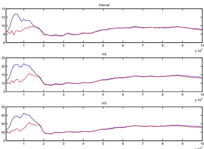
Evaluating the performance of the models to track the properties of the data, looking at Figure 1, the model with financial frictions in some cases better captures the autocorrelation structure of the time series used in the estimation. This is true for output, consumption and investment. It is less clear for the other variables.

Tables 4 and 3 in appendix C, report also the standard deviation and the correlations values. There is not a clear dominance of the model with financial friction in explaining the business cycles. The following charts simple display the autocorrelations in the table.

1 2 3 4 5 0.7 0.8 0.9 1 output 1 2 3 4 5 0.7 0.8 0.9 1 consumption 1 2 3 4 5 0.7 0.8 0.9 1 investment 1 2 3 4 5 0.4 0.6 0.8 1 labour 1 2 3 4 5 0.7 0.8 0.9 1

nominal interest rate

1 2 3 4 5 0.2 0.4 0.6 0.8 1 real wage 1 2 3 4 5 0.7 0.8 0.9 1 inflation

Figure 1: Autocorrelations. Solid line: data autocorrelations. Dashed line: FA

autocorre-lations. Dotted line: NOFA autocorreautocorre-lations.

The convergence analysis, based on specific measure of the parameter vectors

both within and between chains20_{, and obtained running 8 different chains with}

100000 draws for each one of them, suggests that the model without financial friction has less problems, especially in terms of single parameters convergence. Nevertheless, the overall convergence is guaranteed for both eh models.

I can now analyze the estimation results. In table 5, I report the posterior mean and the 95 per cent confidence interval. I will focus first on the key parameter for the financial accelerator, i.e. κ. The estimated value is 0.0548. This value is in line with the calibrated value in BGG and with other results for estimated models for other countries. For instance Did and Christensen estimate it at 0.042 for Canada.

Parameters Posterior mean Confidence interval Posterior mean Confidence interval

without FA with FA σβ 0.0128 0.0106 0.0150 0.0144 0.0102 0.0184 σL 0.0075 0.0059 0.0090 0.0052 0.0044 0.0060 σx 0.0137 0.0116 0.0157 0.0049 0.0036 0.0060 σa 0.0083 0.0073 0.0093 0.0085 0.0074 0.0095 σπ 0.0028 0.0022 0.0033 0.0073 0.0046 0.0097 σr 0.0017 0.0015 0.0019 0.0022 0.0019 0.0025 σg 0.0146 0.0130 0.0162 0.0151 0.0133 0.0167 ρβ 0.8027 0.7630 0.8420 0.8805 0.8414 0.9216 ρL 0.9218 0.8907 0.9537 0.9202 0.8949 0.9465 ρx 0.9461 0.9095 0.9816 0.9972 0.9946 0.9999 ρa 0.7919 0.7487 0.8361 0.7787 0.7277 0.8285 ρg 0.9031 0.8450 0.9624 0.8691 0.7943 0.9416 θe _{0.9750 0.9597 0.9909 0.9766 0.9623 0.9909} κ – – – 0.0548 0.0405 0.0685 ς 0.0218 0.0162 0.0273 0.0076 0.0051 0.0099 φm 0.7927 0.7457 0.8393 0.8610 0.8245 0.8999 Ξ 0.9454 0.8920 0.9980 0.6560 0.5080 0.7905 rπ 1.8045 1.6552 1.9555 1.5125 1.3558 1.6670 ry 0.0860 0.0483 0.1203 0.2144 0.1565 0.2701 ε 0.8471 0.8306 0.8637 0.8575 0.8427 0.8734 h 0.7907 0.7319 0.8495 0.7624 0.6955 0.8244 σl 1.3907 1.2557 1.5241 1.1317 1.0467 1.2083 σc 0.1665 0.0992 0.2341 0.1184 0.0754 0.1602

The mean for the fraction of entrepreneurs who survive, θe_{, is 0.9766. This}

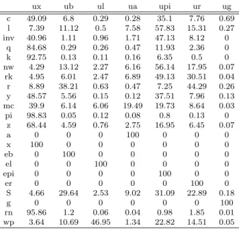
implies an average duration of entrepreneurs of 42 years. The autoregressive coefficients are not surprisingly high, in most cases higher than what expected. The fact that shocks are persistent in the Euro Area is well know and well doc-umented, for instance in Smets and Wouters (2003) and Queijo (2005). Nev-ertheless, in the latter article the estimations of those coefficients are strangely all close to one. More results are more in line with the literature. Contrary, the estimation of the shocks’ standard deviation are more similar to the one ob-tained by Queijo (2005). The variance decomposition presented in the following tablewell shows which shock is more relevant in the Euro Area and which is the most responsible of the variance of the single variables.

ux ub ul ua upi ur ug c 49.09 6.8 0.29 0.28 35.1 7.76 0.69 l 7.39 11.12 0.5 7.58 57.83 15.31 0.27 inv 40.96 1.11 0.96 1.71 47.13 8.12 0 q 84.68 0.29 0.26 0.47 11.93 2.36 0 k 92.75 0.13 0.11 0.16 6.35 0.5 0 nw 4.29 13.12 2.27 6.16 56.14 17.95 0.07 rk 4.95 6.01 2.47 6.89 49.13 30.51 0.04 r 8.89 38.21 0.63 0.47 7.25 44.29 0.26 y 48.57 5.56 0.15 0.12 37.51 7.96 0.13 mc 39.9 6.14 6.06 19.49 19.73 8.64 0.03 pi 98.83 0.05 0.12 0.08 0.8 0.13 0 z 68.44 4.59 0.76 2.75 16.95 6.45 0.07 a 0 0 0 100 0 0 0 x 100 0 0 0 0 0 0 eb 0 100 0 0 0 0 0 el 0 0 100 0 0 0 0 epi 0 0 0 0 100 0 0 er 0 0 0 0 0 100 0 S 4.66 29.64 2.53 9.02 31.09 22.89 0.18 g 0 0 0 0 0 0 100 rn 95.86 1.2 0.06 0.04 0.98 1.85 0.01 wp 3.64 10.69 46.95 1.34 22.82 14.51 0.05

Table 2: Variance decomposition FA in percentage

It is important to stress that the shock on the inflation target and the shock on investments play a quite relevant role for almost ll the variables in explain-ing their variability, while the government expenditure shock is irrelevant for all variables. This latter result is quite common, while the former is different from the decomposition of Smets and Wuoters (the only paper in which a shock on the inflation target is considered); in fact, in their analysis that shock do not assume any active role. This findings may be perhaps explained by the fact the my sample includes many observations after the European Central bank stared to operate, since it is a bank strongly oriented to the inflation stabilization. Dib and Christensen (2007) find similar results in terms of relevance of the invest-ment shocks, first source of variability in the Canadian economy. In the end, Turning to the other estimated parameters, the elasticity of capital price with respect to the investment capital ratio, Ξ, is a bit lower than in Queijo (2005), but still high enough. The estimation of the response inflation to marginal costs is 0.0076, which, given that β is set to 0.99, implies a Calvo parameter equal to 0.99, which in turns means that firms change price every 25 years. This

parameter is usually set at 0.75 (change every year). Smets and Wouter (2003) and Queijo (2005) find that parameter to be 0.90 (change every 2 years and a half) and 0.85 (change every almost 2 years) respectively. The estimation of the model without financial friction gives a more reliable value for ς, giving a Calvo parameter of 0.71. The policy rule parameters do not display any partic-ular strange behaviour. In particpartic-ular, the interest rate smoothing parameter,

φm, and the response of interest rate to the output gap, ry, lay between the

estimation of Smets and Wouters (2003) and Queijo (2005) are in line with the literature, and they are 0.8610 and 0.2144. The mean of the more interesting

parameter rπ is lower than other estimations, but in any acceptable. The

re-maining parameters, related to the consumer side of the economy, i.e. h and

σl, reflect the Euro Area characteristics as in the previous studies, denoting a

persistence in the external habit. Contrary, the estimated mean of σc is much

smaller than other estimations.

5.1

Impulse response functions

To illustrate the different model dynamics implied by the financial accelerator, I plot the impulse response functions of key macroeconomic variables. The most part of these responses are reported in the appendix D and E.

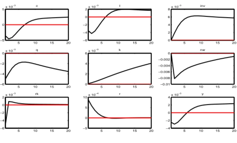
Here, I report the consequences of a monetary policy shock to some variables. Following this shock, the nominal interest rate rises and output, investment, consumption, hours, inflation fall sharply on impact. The basic mechanism of the financial accelerator is evident in the impulse responses. After a tightening in monetary policy, net worth falls, because of the declining return to capital. The external finance premium rises (see appendix D), reflecting the increase in firm leverage. The higher funding cost of purchasing new capital depresses the demand for it, and the expected price of capital persists below its steady-state value. The presence of a financial accelerator mechanism implies a significant amplification and propagation of the monetary policy shock on investment and capital prices.

5 10 15 20 −0.015 −0.01 −0.005 0 c 5 10 15 20 −15 −10 −5 0 5x 10 −3 l 5 10 15 20 −0.02 −0.015 −0.01 −0.005 0 inv 5 10 15 20 −15 −10 −5 0 5x 10 −3 q 5 10 15 20 −0.03 −0.02 −0.01 0 nw 5 10 15 20 −0.01 −0.005 0 y 5 10 15 20 −1.5 −1 −0.5 0x 10 −3 k 5 10 15 20 −1 0 1 2x 10 −3 rn

Figure 2: Variables’ responses to a one standard deviation orthogonalized monetary policy

shock. Percentage deviation from the steady state. Dashed line: without financial frictions. Solid line: with financial frictions.

6

CONCLUDING REMARKS

In this paper I estimated a New Keynesian Dynamic Stochastic General Equi-librium with financial frictions for the Euro Area, along the line of BGG (1999) financial accelerator mechanism. Unlike BGG (1999) I enriched the model with several sources of rigidities and a larger set of structural shocks.

The aim was to investigate, in the context of a structural model, on the relevance of the credit frictions in explaining the business cycles, and the impact of such a relevance on the transmission mechanism of the monetary policy. I found a decisive evidence in favour of the model with financial frictions in fitting data, suggesting that this model is a better representation of the euro area economy. Despite this fact, this model does not explain the business cycle better than the model without financial frictions.

The consequences of the relevance of those frictions is clear for amplitude and persistence of the different shocks hitting the economy. I am particularly interested in the consequences of the monetary policy shocks. They are clearly amplified by the presence of the financial frictions, but the impact on the per-sistence is less relevant.

A

Some steady state values

The real marginal cost is the inverse of the mark-up M C =

µ θ − 1

θ ¶

Referring to the relationship among real wage, marginal cost and productiv-ity of labour I can write

W P = µ θ − 1 θ ¶ (1 − α)Y L And using the condition of the labour supply

µ θ − 1 θ ¶ (1 − α)Y L = Lσl (1 − h) C Rearranging 1 L1+σl = ¡_θ−1 θ ¢ (1 − α) (1−h)C Y

Then, I need the steady state value of the consumption - output ratio C

Y C Y = 1 − I Y − G Y

The steady state value of Q is 1 and the steady state value of I=δK. Sub-stituting in the previous equation

C Y = 1 − δK Y − G Y

Re-arranging and multiplying and dividing by α the last two terms I obtain C Y = 1 − δα αY K −G Y (36)

The steady state of the capital productivity is z = µ θ − 1 θ ¶ αY K Hence equation equation 36 can be written as

C Y = 1 − δα z³ θ θ−1 ´ −G Y (37)

In order to go on I need to specify the the steady state value of the return

on capital Rk_{.I use use two equation to do it (equations ?? and23)}

Rk = SR

where S= is the steady state level of the finance premium. Remembering

that R=(1+i)=(1+r)=1

β (because of the zero inflation steady state), I can write

z as z + 1 − δ = SR z = S1 β − 1 + δ Substituting in equation 37 C Y = 1 − δα ³ S1_β− 1 + δ ´ ³ θ θ−1 ´ −G Y with δ = 0.025, α = 0.3, S=1.02, β = 0.99, θ = 6 and G Y = 0.19521 the

consumption output ratio is

C

Y = 0.692

As a consequence, the investment output ratio is22

I

Y = 0.113

Turning back to the steady state level of L 1 L1+σl = ¡_θ−1 θ ¢ (1 − α) (1−h)C Y L1+σl₌ (1−h)C Y ¡_θ−1 θ ¢ (1 − α) L = " _(1−h)C Y ¡_θ−1 θ ¢ (1 − α) # 1 1+σl With σl= 2 and h=0.6 L = 0.69 21_{See Queijo (2005).} 22_{More formally} I = δK Hence I Y = δ K Y Substituting equation ?? I Y = δ µ θ − 1 θ ¶ α S1+ν β − 1 + δ

References

[1] Adalid, A., G¨unter, C., McAdam, P., Siviero, S. (2005), The

Performance and Robustness of Interest-Rate Rules in Model of Euro Area, ECB’s Working Paper No. 479.

[2] Angelini, P., Del Giovane, P., Siviero, S. and Terlizzese, D. (2002), Monetary Policy Rules for the Euro Area: What Role for National Information?, Temi di discussione, Banca d’Italia. [3] Angeloni, I., Aucremanne, L., Ehrmann, M., Gali, J., Levin, A.,

Smets, F. (2005), Inflation Persistence in the Euro Area: Prelim-inary Summary of Findings, drafted for the Inflation Persistence Network.

[4] Angeloni, I., Kashyap, A. and Mojon, B. (eds.) (2003), Monetary Policy Transmission Mechanism in the Euro Area, Cambridge University Press.

[5] Ball, L. (1999), Policy Rules for Open Economies, in John B. Taylor, ed., Monetary Policy Rules. Chicago, Illinois: University of Chicago Press, 127-144.

[6] Bank for International Settlements (1995), Financial Struc-ture and the Monetary Policy Transmission Mechanism, Basle, Switzerland.

[7] Bernakne, B., Gerltelr, M. and Gilchrist, S. (1999), The Financial Accelerator in a Quantitative Business Cycle Framework, in J. B. Taylor and M. Woodford (eds.) Handbook of Macroeconomics, Amsterdam: North-Holland.

[8] Bernanke, Gerlter and Gilchrist (1996), The Financial Acceler-ator and the Flight to Quality, The Review of Economics and Statistics, vol. LXXVIII, no. 1, pp. 1-15.

[9] Bofim, A. N. and Rudebusch, G. D. (1997), Opportunistic and Deliberate Disinflation Under Imperfect Credibility, Federal Re-serve Bank of San Francesco.

[10] Breuss, F. (2002), Was ECB’s monetary policy optimal?, Atlantic EconomicJournal, 30, 298-320.

[11] Bryant, R. C., Hooper P. and Mann C., eds., (1993), Evaluating Policy Regimes: New Research in Empirical Macroeconomics, Brooking Institute, Washington, DC.

[12] Casares, M. (2006), ECB Interest-Rate Smoothing, International Economic Trends, Federal Reserve Bank of ST. Louis.

[13] Castelnuovo, E. and Surico, P. (2004), Model Uncertainty, Op-timal Monetary Policy and the Preferences of the Fed, Scottish Journal of Political Economy, 51(1), 105-126.

[14] I. Christensen, A. Dib, The financial accelerator in an estimated New Keynesian model, Review of Economic Dynamics (2007), doi:10.1016/j.red.2007.04.006.

[15] Christiano, Motto, and Rostagno (2004), The Great Depression and the Friedman-Schwartz Hypothesis,” NBER working Papers 10255.

[16] Clarida, R., Gali, J., Gerlter, M. (1999), The Science of Monetary Policy: A New Keynesian Perspective, NBER Working Paper. [17] Clarida, R., Gali, J., Gerlter, M. (2000), Monetary Policy Rules

and Macroeconomic Stability: Evidence and Some Theory, The Quarterly Journal of Economic.

[18] Clausen, V. and Hayo, B. (2002), Monetary Policy in the Euro Area – Lesson from the First Five Years, Center for European Integration Studies Working Paper.

[19] Coenen, G. and Wieland, V. (2000), A Small Estimated Euro Area Model with Rational Expectations and Nominal Rigidities, ECB Working Paper No. 30.

[20] Di Bartolomeo, G., Rossi, L. and Tancioni, M (2005), Monetary Policy Rule-of-Thumb Consumers and External Habits: An In-ternational Empirical Comparison, mimeo.

[21] Dieppe, A., K¨uster, K. and McAdam, P. (2004), Optimal

Mone-tary Policy Rules for the Euro Area: An Analysis Using the Area Wide Model, ECB Working Paper No. 360.

[22] European Central Bank (2004), The Monetary Policy of the ECB. [23] European Central Bank (October 2001), Monthly Bulletin. [24] Fagan, G., Henry, G. and Mestre, R. (2001), An area-wide model

(awm) for the Euro area, ECB’s Working Paper No. 42.

[25] Fendel, R. M. and Frenkel, M. R. (2006), Five Years of Single European Monetary Policy in Practice: Is the Ecb Rule-Based?, Contemporary Economic Policy, 24(1), 106-115.

[26] Fernandez-Villaverde, J. and Rubio-Ramirez, J. (2001), Compar-ing Dynamic Equilibrium Models to Data, mimeo.

[27] Four¸cans, A. and Vranceanu, R. (2002), ECB Monetary Policy Rule: Some Theory and Empirical Evidence, ESSEC Research Centre Working Paper No. 02008.

[28] Gali, J. (2001), European Inflation Dynamics, European Eco-nomic Review, 45, 1237-1270.

[29] Gal´ı, J., Gerlach, S., Rotemberg, J., Uhlig, H. and Woodford, M. (2004), The monetary policy strategy of the ECB reconsidered: Monitoring the European Central Bank 5. CEPR.