2 An Introduction of the Theory Used in this Thesis

2 An Introduction of the Theory Used in this

Thesis

The theory on which project is based is not well defined; in fact, there are only few references in literature about side entry impeller and non-standard geometries. Hence, the theory described below is often about a standard geometry when there are inadequate references available. An introduction to used basic concepts in this thesis will be initially presented and then the scale-up/down rules are explained.

2.1 Power Consumption

The cost of a process depends on the power consumption. In order to ensure an optimum productivity, energy consumption must be optimised.

2.1.1 Impellers in Ungassed Newtonian Fluids

The power drawn by a rotating agitator is one of the most important parameter for the design of mechanically agitated vessels and for the understanding of all the developed processes. Although the recent literature has given specific detail for the power drawn for many impellers, the most generally accepted evaluation for the power consumption was found at the 1950’s, and it is shown in Eq. 2-1:

5 3

D N

P∝ ⋅ Eq. 2-1

where the power drawn P is related to the impeller diameter D and the rotational speed N. As explained by Bates et al.5,6 _{a dimensional}

analysis can be obtained from Navier-Stokes equation of motion, and shows that:

0

,

,

₂ 2

=









∆

=

v

p

Lg

v

vL

F

ρ

µ

ρ

Eq. 2-2 where

v

=

velocity; = L a characteristic length, = ∆p pressure difference.

The first group in Eq. 2-2, is the Reynolds number and represents the ratio of inertial forces to viscous forces. Substituting L with the

diameter of the impeller, D, and

v

with

ND

, where

N

is the impeller rotational speed, the Reynolds number can be written as:

µ

ρ

2

Re

=

ND

Eq. 2-3

The group

v /

2

Lg

is known as Froude number and represents the ratio of inertial to gravitational forces. Making the previous substitutions into this group, the following equation is obtained:

blades could be integrated to give torque acting on the impeller. In fact, the power can be calculated directly from the total torque and the rotational speed of the impeller as follows:

NM

P

=

2

π

Eq. 2-5

Where P is the power draw, N and M are the rotational speed and the shaft torque respectively. It can also be shown that ∆p and power

are related by 3 ND P p = ∆ Eq. 2-6

At this point the last group of Eq. 2-2, evolves in the following number, and is known as power number:

5 3 D N P Po ρ = Eq. 2-7

For usual standard geometries it has been found that the trend of the

Po

against the

Re

or the rotational impeller speed has got the behaviour shown in Figure 2-16_{. This curve can be divided in three}

different sections: the first one where

Po

is inversely proportional to

Re

, typical behaviour of the laminar region, then follows a transitional section till the turbulent flow is established, where

Po

can be assumed constant.

The last parameter used for ungassed system analyzed is known as specific energy dissipation rate,

ε

_T, that is the ratio between the power absorbed,

P

, and the volume of the vessel,

V

. Since in the turbulent region the Po is constant the

ε

_Tmight be expressed as:

V

D

N

Po

3 5 T

ρ

ε

=

Eq. 2-8

The ratio

ε

_T is expressed in [W/m3_].

NM

P_g =2π Eq. 2-9

Where the subscript

g

defines the gassed power. As well as the gassed power, the gassed power number is also defined, and its expression is

To compare different systems, in gas power studies, the power ratio

Po

Pg / is reported, where

Po

is assumed constant, against the

Reynolds number and gas flow rate.

As like as all the other parameters, for gassed system also the

ε

_Twill change in

( )

ε

_{T g}. However, it should be noticed that for this specific condition the

Po

g is never constant so the

( )

ε

T _gcan not be expressed

in absolute value, but it has defined for every different rotational impeller rate. 5 3 g

D

N

P

Po

L g

ρ

=

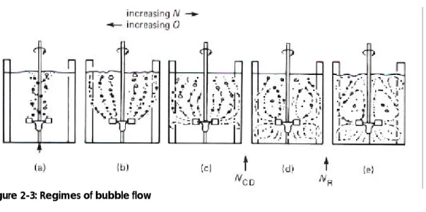
Eq. 2-10

the different gas flow patterns with changing speed as identified by Nienow et al.8 _{and by Chen et al.}9_{. These are shown in Figure 2-3}10_.

These flow patterns can be associated closely with a graph of Po_g/Po

against gas flow number, 3

/ ND

Q

_g , with increasing

N

when

Q

g is held

constant. A characteristic example is shown in Figure 2-410_{. At lowest}

N

(region a) the gas passes through the agitator without any effects and the liquid flows around the outer part of the blades undisturbed by the gas. Thus, the gassed power is not much less than the ungassed. As

N

increases, gas is captured by the vortices behind the impeller blades (large cavity, see Figure 2-26_{) and dispersed;}

_P

g

decreases. Further increase of

N

reduces the cavities and changes their form to ‘vortex’ cavities. The curve passes through a minimum, at a speed,

N

CD, the minimum speed to just completely disperse the

gas. It then rises while small recirculation patterns start to emerge (region d). The maximum corresponds to the speed,

N

R, at which

gross recirculation of gas back into the agitator sets in

2.2 Mixing Time

Another parameter, which is related with the power draw, is the mixing time. This is the time needed by a system to have a complete circulation, e.g. when the whole bulk is completely stirred. This aspect, also if is not explained by any laws, is fundamental to give an idea about how the system is working; in fact, circulation times are measures of average velocity, bulk motion or convective transport generated by liquid pumping of the impeller11. The power drawn is