A computational framework for modeling, simulation and optimization of energy supply chains

(1)

POLITECNICO DI MILANO

DIPARTIMENTO DI ENERGIA

DOCTORALPROGRAMMEIN ENERGY ANDNUCLEARSCIENCE AND

TECHNOLOGY CYCLEXXXI

A COMPUTATIONAL FRAMEWORK FOR

MODELING, SIMULATION AND

OPTIMIZATION OF ENERGY SUPPLY

CHAINS

Doctoral Dissertation of:

SHIYU CHEN

Supervisor:

Prof. ENRICO ZIO

Co-supervisor:

Dr. WEI WANG

Dr. MICHELE COMPARE

Tutor:

Prof. FRANCESCO DI MAIO

The Chair of the Doctoral Program:

Prof. VINCENZO DOSSENA

(2)

(3)

ACKNOWLEDGEMENTS

I would like to express my special appreciation and thanks to my supervi-sors: Prof. Enrico ZIO, for his insightful guidance, strong sense of respon-sibility, great technical supports, numberless discussions throughout all the course of this thesis. His blessing, help and guidance on both research as well as on my career are priceless. It is a pleasure and a great honor to pursue a Ph.D. degree under his supervision.

I would like to express my sincere appreciation and gratitude to the Ph.D. programme “Energy and Nuclear Science and Technology” in De-partment of Energy, Politecnico di Milano, and to the program coordina-tors, Prof. Vincenzo Dossena and Prof. Carlo Enrico Bottani, for a five-year hosting.

I would like to express my special appreciation to my co-supervisor Dr. Wei WANG, for his encouragement and help when I had rough period time during my Ph.D. career. I would like to express my sincere gratitude to my tutor, Prof. Francesco DI MAIO, for his patience and help of my activities at Politecnico di Milano.

I would also like to take this opportunity to thank all my friends/col-leagues in LASAR research group (Laboratory of signal and risk analy-sis): Prof. Piero BARALDI, Marco RIGAMONTI, Sameer AL-DAHIDI, Francesco CANNARILE, Zhe YANG, Alessandro MANCUSO, Edoardo TOSONI, Mingjing XU, Seyed MOJTABA HOSEYNI, Federico ANTONE-LLO, Luca PINCIROLI, Dario VALCAMONICO, Bingsen WANG, Zhao-jun HAO, Mei CHEN, Xuefei LU, Ahmed SHOKRY and Michele COM-PARE. It has been a great pleasure to work with them during the last five

(4)

ited LASAR group: Masoud NASERI, Tao TAO, Youhu ZHAO, Huai SU, Xiaoyu CUI, Tongyang LI, Tongdian WANG, Miao YU, Yu YU, Yanhua ZOU, Haifeng GAO, Yongcheng XU, Yue LIU, Jiayan ZHOU, Yan SHI, Zhiyao ZHANG, Kun MA, Shaomin ZHU, Yang LI, Zhe TONG, Xueyi LI, Yaping LI, Wanqing SONG and Bokai ZHENG.

I would like to thank my parents for their everlasting love and financial support.

At last, I would like to thank the China Scholarship Council for granting me the scholarship to pursue the Ph.D. degree.

(5)

ABSTRACT

E

NERGY Supply Chains (ESCs) are complex systems made up of a number of heterogeneous components/agents interacting with each other, the environment, its hazards and threats. The components/a-gents are structured in a hierarchical system, within which they operate and cooperate in a balanced transaction environment to realize the maximiza-tion of the benefits, under various environmental and safety constraints. ESCs significantly contribute to the sustainment of many industrial areas, such as biomass, oil and gas, chemical processing, sustainable and renew-able energy, etc.

However, ESCs are challenged by multiple sources of uncertainties and risks. Uncertainties exist in supply and demand, propagate through the in-teractions over the whole ESC and influence the agents profits and the ESC operations. Due to the uncertainties, the risk of supply failure is difficult to predict. In such situation, ESCs must offer enhanced flexibility, innova-tive connectivity and communication, to guarantee an orderly and healthy supply management, so as to sustain the operation of the energy industry.

The objectives of the Ph.D. work are to develop a modeling framework for ESC process modeling simulation and optimization, which includes: 1. ESC modeling to identify, understand and analyze the complex interac-tions and for the evaluation of the resilience of ESCs. 2. ESCs efficient production planning optimization under multiple sources of uncertainty. 3. ESCs production planning considering risk of supply failure. 4. Solving the Many-objective Optimization Problem (MaOP) caused by the different agents for efficient production planning of ESCs.

(6)

dustry, capturing the peculiarities of its diverse interacting elements, such as plants, refineries, storages, etc. Different disruption scenarios and recovery strategies are considered in the Agent-based ESC model for investigating the relevant factors influencing ESC resilience.

With respect to the objectives 2 and 3, a simulation-based Multi-Objective Optimization (MOO) framework for ESC production planning is devel-oped. The ABM simulation is embedded into a Non-dominated Sorting Genetic Algorithm (NSGA-II) is then adopted for identifying the Pareto solutions. For ESCs with uncertainties and changing structures, the ESC total profit is maximized and the disequilibrium among the agents’ profits is minimized. Moreover, considering disruption risks, the ESC total profit is maximized and ESC risk under uncertainties is minimized.

Furthermore, an improved Cooperative Co-evolutionary Particle Swarm Optimizer (CCPSO) is proposed to solve the Many-objective Optimization Problem (MaOP) in the agent-based ESC model. The variables are decom-posed into different species based on agents relationships and allowed to evolve independently during the optimization process. Each species has its own repository to keep a historical record of the nondominated vectors in which the solutions are evaluated and updated by cooperating with other species. The effectiveness of CCPSO is proven by test functions and a case study.

KEYWORDS

Energy Supply Chain; Oil and Gas Supply Chain; Agent-based Mod-eling; Multi-objective Optimization; Uncertainty; Risk; Changing Struc-ture; Monte Carlo Simulation; Non-dominated Sorting Genetic Algorithm; Many-objective Optimization Problems (MaOPs); Co-evolutionary Algo-rithm; Multi-objective Particle Swarm Optimization (MOPSO); Coopera-tive Co-evolutionary Particle Swarm Optimizer (CCPSO).

(7)

List of Tables

Table 1.1 The related factors considered in each chapter . . . . 15 Table 2.1 The resilience loss comparing with taking the safety

inventory to mitigate the influence of disruption . . . 30 Table 2.2 The resilience loss comparing with taking the flexible

production capacity to mitigate the influence of disruption . 30 Table 3.1 The setting of the parameters for the ABM-MOO . . 40 Table 3.2 The values of the orders and prices limitations . . . . 40 Table 3.3 The values of the unit prices ol+1,v_l,v 0 (¤/ton) for the

other cost from al+1,v0 to a_l,v . . . 41

Table 5.1 The variable number and the objective number of ZDT2 and DTLZ2 . . . 70 Table 5.2 The parameter settings of CCPSO and MOPSO for

ZDT2 . . . 70 Table 5.3 The parameter settings of CCPSO and MOPSO for

DTLZ2 . . . 71 Table 5.4 The setting of the parameters for the ABM-MOO . . 72 Table 5.5 The values of the orders and prices limitations . . . . 72 Table 5.6 The values of the unit prices ol+1,v_l,v 0 (¤/ton) for the

other cost from al+1,v0 to a_l,v . . . 73

Table 6.1 Original contributions of this Ph.D. work . . . 76 Table 6.2 Perspectives of this Ph.D. work . . . 77

(12)

(13)

List of Figures

Figure 1.1 ESC models . . . 7

Figure 1.2 The framework of our agent-based ESC modeling . 14 Figure 1.3 The structure of the PhD thesis . . . 16

Figure 2.1 ESC structure . . . 20

Figure 2.2 The ABM-ESC model . . . 21

Figure 2.3 The process of sending orders . . . 21

Figure 2.4 The process of receiving orders and choosing de-mander(s) . . . 23

Figure 2.5 The process of response . . . 25

Figure 2.6 The process of selling production . . . 26

Figure 2.7 Resilience loss . . . 27

Figure 2.8 The resilience loss in the scenario S1 and S2 . . . . 28

Figure 2.9 The resilience loss in the scenario S3 and S4 . . . . 29

Figure 2.10 The resilience loss in the scenario S5 . . . 29

Figure 3.1 The flowchart of the ABM-MOO framework . . . . 39

Figure 3.2 Sensitivity for the profit and the disequilibrium . . . 42

Figure 3.3 Sensitivity on the order amounts for the profit . . . . 43

Figure 3.4 The Pareto front . . . 44

Figure 3.5 The values of the orders (ton) sent by the agent al,v for getting Pareto solutions H1, H2 and H3 . . . 45

Figure 3.6 The values of prices (¤/ton) for getting H1, H2 and H3 . . . 46

(14)

Figure 3.7 The profit and the disequilibrium of the profit for each layer considering variables of H1 . . . 47

Figure 3.10 The ESC total profits obtained from the re-inputs of H1, H2 and H3 . . . 52

Figure 3.11 The disequilibrium for each layer considering vari-ables of H1, H2and H3 . . . 52

Figure 3.12 Pareto fronts in MC simulations . . . 53 Figure 4.1 Distribution of sending production loss . . . 56 Figure 4.2 The flowchart of the ABM-MOO framework . . . . 59 Figure 4.3 The Pareto front with the best-compromised solution 60 Figure 4.4 The cost frequency distribution under the ESC

nor-mal state . . . 60 Figure 4.5 The cost frequency distribution with the ESC

dis-ruption risk . . . 61 Figure 4.6 The cost frequency distribution with the ESC

dis-ruption risk after optimization . . . 61 Figure 5.1 The Pareto front of CCPSO and MOPSO for ZDT2 . 69 Figure 5.2 The Pareto optimal solutions of CCPSO and MOPSO

for DTLZ2 . . . 69 Figure 5.3 The framework for MaOP in agent-based ESC

mod-eling . . . 70 Figure 5.4 The framework for MaOP in agent-based ESC

mod-eling case study . . . 71 Figure 5.5 The Pareto optimal solutions . . . 73 Figure 5.6 The HV metric values . . . 74

(15)

LIST OF ACRONYMS

ABM Agent-based Modeling AHP Analytic Hierarchy Process

CCGA Cooperative Co-evolutionary Genetic Algorithm

CCPSO Cooperative Co-evolutionary Particle Swarm Optimizer CEA Co-evolutionary Algorithm

CPSO Cooperative Particle Swarm Optimizer CVaR Conditional Value at Risk

DEA Data Envelopment Analysis DES Discrete Event Simulation DS Dynamic Simulation EA Evolutionary Algorithm ESC Energy Supply Chain GA Generation Algorithm

GIS Geographical Information System LP Linear Programming

MaOP Many-objective Optimization Problem

MC Monte Carlo

MCDM Multi-Criteria Decision Making MILP Mixed-Integer Linear Programming MINLP Mixed-Integer Nonlinear Programming MOO Multi-objective Optimization

(16)

MOPSO Multi-objective Particle Swarm Optimization NLP Nonlinear Programming

NSGA-II Non-dominated Sorting Genetic Algorithm PSO Particle Swarm Optimizer

(17)

SECTION I: GENERALITIES

This part of the dissertation introduces the context of the research, its rel-evance, the state-of-the-art methods, the challenges that are addressed and the research objectives. Furthermore, it briefly describes the developed methods and the applications carried out for their validation.

(18)

(19)

CHAPTER

1

Introduction

1.1

ESC

ESCs are complex systems made up of numerous components/agents in-teracting with each other, the environment and its hazards. An ESC may be view as an network of components/agents (e.g. retailer, refinery, stor-age, crude oil producer) and transportation (e.g. pipe line, crude oil tranker, truck) [1, 2]. ESCs management is a complex process because of many factors involved.

Energy companies in the ESC have to face uncertainties and risks. The demand, manufacturing and supply uncertainties involving the unknowns related to product characteristics are the major sources of uncertainties [3]. Along with these uncertainties, the considerations assigned to risk have grown. For example, new, unconventional sources of energy such as shale gas, tight oils, coal seam gas and oil sands are heavily influencing the en-ergy market, while requiring the ESC to still offer reliable and high quality of service, but also to be more flexible and resilient. Yet, price volatility and increasing operating costs are causing energy companies to scrutinize the existing sourcing strategies and the costs associated with the VMI, con-signments, etc. [4]. Moreover, the number of terroristic attacks

(20)

impact-ing on supply chains has increased steadily over the past decade, reachimpact-ing 3299 attacks in 2010 [5]. These attacks entail possibly disastrous conse-quences on societies, which nowadays depends on the effective functioning of complex network systems (e.g., power supply networks, transportation networks, etc.) [6, 7]. Setting measures for withstanding the attacks has also led to an increment in the operation costs of ESC. These considera-tions justify the increasing interest in analyzing the ESC risk which could be categorized into two types: disruption risks and operational risks [8, 9]. The disruption risks are related to circumstances such as natural disaster, terrorist attacks and labor strikes, while operation risks are caused by high uncertainty and unbalance between supply and demand [10, 11]. The risk is hard or even impossible to be predicted which makes the ESC disrupted and influences the ESC function [12].

Except for the influencing of uncertainties and risks, the structure of ESC is complex. The components/agents such as crude oil producers, re-fineries, storages in ESC are physically and functionally heterogeneous and organized in a hierarchy of subsystems, what happens to one individual will directly or indirectly affect others and spread through the whole ESC. For example, if the disruption happens on ESC, energy company may lose a drilling day waiting on mud system arrival, lose a week of production be-cause of a treating chemical stock out, or miss a day of retail sales bebe-cause the refinery production schedule was not balanced with demand. Secondly, the interaction between components/agents is complex and dynamic which is difficult to describe by traditional analytical methods [13].

According to the system and complexity’s theories, we view an ESC as a complex system or in other words, it is a system in a complex system-of-system. Under such background, we focus our research on modeling and optimizing ESC which are important and significant issues and have been paid more and more attention but they are challenged by diverse factors.

1.2

Challenges in ESC

I. Uncertainty and risk challenge: The phenomena of uncertainties and risks needs to be addressed when designing ESC. Thus, there is a need to develop novel hybrid approaches combining the strengths of multiple techniques of optimization under uncertainties and risks [1].

II. Modeling challenge: This challenge arises from the need to accu-rately model materials and information flows in ESC [1]. Due to the com-plex features in ESC, identifying, understanding and analyzing the comcom-plex interactions between agents represent a challenge to ESC.

(21)

1.3. Research Objectives of The Thesis

III. Optimization challenge: The efficient operation of energy com-panies’ production planning is required. However, it is difficult and chal-lengeable for ESC to get the production planning optimization in complex ESC environment.

III. Computation challenge: There are many agents (e.g. retailer, refinery, storage) whose variables and objectives are independent, so the MaOPs are caused in ESC which are difficult to be solved by traditional EA. It rises another challenge to ESC.

1.3

Research Objectives of The Thesis

In this context, considering the challenges mentioned above, we aim at solving the problem of modeling, analyzing, designing ESC in uncertain and risky environment. The research objectives focus on four of the most challenging problems:

I. Modeling to evaluate the resilience of the ESC

From the complexity of agents’ interdependences, risk scenarios can originate in an unpredictable way, threatening the normal operation of the entire ESC and endangering its supply capability. New methodologies are, then, being developed for carrying out ESC risk and resilience analyses. In this study, we rely on ABM to build a multi-layer ESC modeling for an-alyzing its resilience. Every element in the ESC is simulated as an agent implementing basic functions like sending and receiving orders, and pro-ductions. We simulate different disruption scenarios and recovery strategies to investigate the essential factors influencing the resilience of the overall ESC.

II. Designing efficient energy companies’ production planning Energy production companies have to make planning decisions to sat-isfy the customers uncertain demands and to maximize their own profits. In this work, we propose a simulation-based MOO framework for the efficient management of the ESC sustaining production. The ESC agents interaction is uncertain and the ESC structure can dynamically change. ABM is used to model and simulate the agents actions and behavior, and the ESC transac-tion processes. The simulatransac-tion is embedded into an NSGA-II optimizatransac-tion scheme for identifying the Pareto front of solutions for which the ESC total profit is maximized and the disequilibrium among the agents profits is mini-mized. Based on the Min-Max method, a single best compromised solution is identified. Finally, the MC simulations approach is used to operational-ize the proposed ABM-MOO framework in presence of the uncertainty that affects the ESC.

(22)

For demonstration, we consider an oil and gas ESC modeling with five layers, including crude oil producers, storages, refineries, terminal storages and retailers. The results show that the proposed framework enables the op-timization of the ESC planning, while taking into account multiple sources of uncertainty and the structure dynamics that challenge the ESC operation. III. Optimizing the planning of ESCs considering the disruption risk

The planning of an ESC aims at maximizing the benefits of the ESC agents, while satisfying the demands of the customers [14, 15]. Demand variability and supply disruption, originating from the connectivity between supply and demand, can disturb the agents interactions and impair the agents management [16]. In this study, we propose a risk-based optimization ap-proach for the management of ESC. We introduce a CVaR measure with the purpose of measuring and controlling the risk to the ESC management. The NSGA-II is performed to search for the solutions optimal with respect to the maximization of the ESC total profit and the minimization of the risk under uncertainties.

For demonstration, an application is carried out considering a specific oil&gas ESC modeling with five layers, including crude oil producers, stor-ages, refineries, terminal storages and retailers. Results show that the opti-mization approach enables the trade-off between the ESC optimal planning and the source of risk that it is subjected to.

IV. Solving Many-objective Optimization Problems (MaOPs) in ESC In ESCs, multiple agents proactively interact and cooperate in a coor-dinated production process, where each of them aims to grab the maximal own profits. In this study, we propose a cooperative co-evolutionary ap-proach to solve such an ESC Many-objective Optimization Problem (MaOP) where the agents own profits are maximized. The autonomous behavior of the ESC agents and the interactive transaction processes are modelled in the context of ABM. A CCPSO algorithm is embedded into ABM for iden-tifying the Pareto Front (PF). The effectiveness of the proposed approach is verified by the test functions.

For demonstration, we also illustrate the proposed approach by consid-ering an oil and gas ESC model with five layers, including crude oil produc-ers, storages, refineries, terminal storages and retailers. The results show that the proposed CCPSO enables the many-objective optimization for the efficient production planning of the ESC, whilst taking into account multi-ple sources of uncertainty and the structure dynamics challenging the ESC operation balance.

(23)

1.4. State-of-the-Art Literature Review on ESC Models

Figure 1.1: ESC models

1.4

State-of-the-Art Literature Review on ESC Models

A variety of models have been used to model and describe the character-istics of an ESC, and they can be identified into three categories based on model types, as shown in Figure 1.1.

Mathematical programming has been widely used to solve the problem of the optimal design of ESC networks. A variety of techniques have been applied in this context, like LP, MILP, NLP and MINLP, etc. For example, a simple LP model is presented for the optimal allocation of palm biomass supply chain [17]. Bittante et al. [18] have applied MILP to find the supply chain structure that minimizes costs associated with fuel procure-ment. Robertson et al. [19] have used NLP model to solve refinery pro-duction scheduling and unit operation optimization problems. In Ref.[20], a two-stage stochastic MINLP model combined with chance constraint is proposed to minimize the total cost of producing electricity from woody biomass in a four-level integrated bioenergy supply chain. Although appli-cable to the treatment of problems involving blending, continuous flow pro-cessing, production and distribution, strategic/tactical planning, etc., math-ematical programming models are not flexible in dealing with the stochas-ticity, uncertainty and complexity of structure and interaction typically en-countered in supply chains [21, 14].

Analytical models build on mathematical expressions and numerical models characterize the ESC behavior, and find solutions to ESC manage-ment problems by use of, for example, Game theory, MCDM (including DEA, AHP), etc.[22]. In Ref.[23], authors proposed a novel Game-theory-based stochastic model for optimizing decentralized supply chains under

(24)

uncertainty. Optimization of renewable power sources has been tackled with a fuzzy MCDM technique based on cumulative prospect theory in Ref.[24]. A DEA model has been used to reduce the complexity of solving the proposed model in the literature [25]. In Ref.[26], AHP combined with a fuzzy set theory enhances the reliability of the sustainable results along different stages of petroleum refinery industry projects. Analytical model-ing can be used to evaluate and improve the performance of an ESC, but has strong limitation in the description of realistically complex supply pro-cesses including stochastic and dynamic structures, uncertainty and partial information sharing [13].

Simulation models, e.g. DES and DS, have been developed to explore the behavior of agents in ESC, with the further goals of evaluation [27], analysis and optimization [28], risk management [29], and so on. For ex-ample, Windisch et al.[28] have applied DES to simulate the raw material planning in an energy wood supply chain. Becerra-Fernandez et al. [30] have proposed a DS model for assessing alternative security of supply pol-icy along the natural gas value chain. The modeling benefits and the large computational capacities make simulation models increasingly attractive for the modeling of ESC realistic problems.

ABM provides another way to model and simulate ESC, also applicable to continuous processes [31, 32] and also applied to various types of supply chains. For example, Guo et al. [33] applied ABM to build an integrated system modeling framework for a resource-food-bioenergy nexus applica-tion. Raghu et al. [34] relied on ABM and GIS to assess the environmental impact on the forest biomass supply chain. Moncada et al. [35] developed a spatially explicit agent-based model to analyze the impact of different blend mandates and taxes levied on investment in processing capacity, and on production and consumption, of ethanol in the biofuel supply chain. In Ref.[36], the authors used ABM to analyze the evolution of biofuel produc-tion and producproduc-tion capacity.

These published researches confirm that ABM can be effectively used for modeling, simulating, assessing and analyzing ESC but, rarely it has been used in optimizing ESC operations. To the authors’ knowledge, no study has yet attempted to solve ESC planning problems by using ABM within an optimization framework and also considering demand and sup-ply uncertainties and structure dynamics at the same time. This is done here, thanks to the capability of ABM in dealing with complex production processes and service problems under uncertainty.

(25)

1.5. Overview of The Proposed Framework

1.5

Overview of The Proposed Framework

1.5.1 Simulation-optimization framework

To the best of my knowledge, the hybrid simulation-optimization frame-work is first proposed by Subramanian, pekny and Reklaitis. They present the hybrid simulation-optimization framework to assess the uncertainty and control the risk in the pipeline [37]. Now, some researches have been done in this area.

For instance, Jung et al.[37] use a simulation-based optimization ap-proach to determine the safety stock level and scheduling applications. Nikolopoulou and Ierapetritou [38] combine methematical progamming and simulation model to minimize the summation of production cost, trans-portation cost, inventory holding and shortage costs. Sahay and Ierapetri-tou propose a hybrid simulation-based optimization framework to solve the two-stage optimization problem [39].

In the hybrid simulation-based optimization, the method can be divided into phase: simulation phase and optimization phase. In the simulation phase, ABM is a good modeling to give a realistic representation of ESC. In the optimization phase, finding the high-quality solutions is the most important task [38]. This demand leads to various optimization algorithms applied in this field. The choice of optimization algorithm is important because it influences the effect and efficiency of the results [40]. Realistic ESC problems have multi-objective or even many-objective which contains more than three objectives. EA working with a population of solutions naturally offers a suited algorithm to solve such optimization problems [41, 42].

1.5.2 ABM

Although analytical model has been proven useful in many fields [38], it still has some limitation in describing some complex phenomenon from system perspective. ESC is a complex system which is dynamic, has com-plex structure and contains plenty of uncertainties, so traditional analytical model is confining in modeling ESC [13]. Overcoming these shortages of analytical model, ABM shows its advantage in modeling ESC.

Firstly, ABM is good at dealing with complex. Some systems are too complex for us to adequately model. However, Agent-based model is “bot-tom up” modeling approach which can model the complexity arising from individual actions and interactions [31, 43]. Secondly, ABM is easy to operate. ABM just needs to describe basic behaviors and interactions from

(26)

individuals which are formalized by simple equations, (decision) rules such as if-then kind of rules or logical operation [44]. Moreover, it is easy to im-plement individual variations and random influences(stochasticity) in ABM [44]. Thirdly, ABM is observable. The Agent-based simulation approach is a method that allows to observe the behaviors through time and the dy-namics of the supply chain from interactions [45].

Due to these advantages, at present, ABM is widely used in modeling supply chain. For example, ABM is used in Wu et al. [46] to investigate re-tail stockouts. In this literature, authors develop an Agent-based simulation model to understand the influence of different stockout length for different products and the response from the retailer and the manufacturers of the product. Fox et al. [47] rely on ABM to manage perturbation in the supply chain with complex cooperative work. Julka et al. [48] rely on ABM to model, monitor, and manage supply chains. Authors view elements in the supply chain as entities, flows and relationships. Entities are modeled as agents and flows are modeled as objects. The authors use two case studies to illustrate the framework. Finally, Gjerdrum et al. [49] develop a supply chain by applying ABM. In this literature, authors model every different role in the supply chain as an agent. All the agent types include customer, external logistics, warehouse, internal logistics, factory, spot market and transportation. In the experiment, authors investigate how optimal schedul-ing influence the behavior.

ABM offers possible way to control complex agents’ behavior and their interaction in ESC. In this thesis, ABM is implemented in the software ANYLOGIC, which is exported as a jar file and then, imported and run in ECLIPSE.

1.5.3 Evolutionary algorithm

EAs are the algorithms that are based on the evolution of the species [50]. EAs use bio-inspired mechanisms, including mutation, crossover, selection and survival of the fittest to refine a set of solution candidates iteratively [51]. GA is one typical algorithm of EAs.

In GA, a set of candidate solutions represented as chromosomes is gen-erated. By selection, crossover, mutation the GA iteratively eliminates poor solutions and the solutions with high fitness value have high probability to survive in the next generation. Consequently, GA is convergent to overall good solutions.

In the field of supply chain, many problems are solved by applying GA. For instance, Altiparmak et al. apply GA to solve a supply chain network

(27)

1.5. Overview of The Proposed Framework

design problem in order to minimize the total cost and the capacity utiliza-tion ratio in supply chain network and maximize the total customer demand (in %) [52]. Naso et al. propose a novel meta-heuristic approach based on GA to solve supply chain scheduling problem [53]. In literature [54], a heuristics based genetic algorithm is proposed by Kannan, Sasikumar and Devika to solve the optimum usage problem of secondary lead recov-ered from the spent lead-acid batteries for producing new battery. Yeh and Chuang use the multi-objective GA approach to solve the partner selection problem in green supply chain. GA is considered as a primary tool to solve many multi-objective problems in supply chain.

In spite of the liveliness of research applying GA in supply chain, only a few papers combine GA and AMB to solve problems in supply chain. Considering the good ability of ABM in dealing with complex problem un-der uncertainty. Simulation-based optimization combining GA and ABM offers a possible way to solve variety of problems in supply chain, more so in case of ESC [55].

1.5.4 CEA

CEA is similar to EA but CEA co-evolves sub-populations of individuals representing different parts of the global solution instead of evolving one population of similar individuals representing a global solution [56]. There are several advantages of CEA [57]: For example, decomposed problem allows calculating in parallel which speeds up the optimization process. Moreover, separated species help to maintain good solution diversity [58], increase the robustness against the modules’ errors and failures and enhance the reusability in dynamic environments [59].

According to the relationship between sub-populations, CEA can be di-vided into two main types: the competitive CEA and the cooperative CEA [56]. In competitive CEA, individual competes with others so it usually contains the whole problem and variables but individual in cooperative CEA decomposes the problem and has partial variables.

In the competitive CEA, individuals in the populations compete among themselves, characterizing the classical predator-prey or an arms race co-evolution [60], and usually individuals contain the whole variables. The fitness of an individual is the result of a series of encounters with other individuals from other species [61, 56].

A variety of MaOPs have been solved by the competitive CEA. The competitive CEA is firstly proposed in Ref.[62], where two sub-populations are considered as the hosts and the parasites to evolve simultaneously and

(28)

interact through their fitness function. The competitive CEA can be imple-mented in a predator-prey-like way, in order to imitate the competitive be-havior between two sub-population, for example, a biogeography optimiza-tion in the constrained design of a brushless dc wheel motor [63]. Whereas, another way based on competitive fitness is adopted in the arms race forms of all-againts-all, bipartite, all versus best, tournament, k-random and so on [56, 64, 65, 66, 67].

For the cooperative CEA, the fitness of an individual is the performance collaborating with other individuals from other species[68, 69] in which individuals usually contain partial variables. Comparing with competitive CEA, the species in cooperative CEA has to cooperate with others to as-semble the whole variables, and then, the fitness value can be calculated.

Potter and De Jong [69], for the first time, proposed a CCGA approach in which the decision variables are divided into the small size species, evolved independently, evaluated cooperatively. Bergh and Engelbrecht proposed two new cooperative PSO models: CPSO-Sk and CPSO-Hk, by

applying Potter’s co-evolutionary technique to the PSO [70]. It is proven that the PSO-based algorithms surpass the performances of the GA-based algorithms on the test problem [70]. Besides, some other researches are proposed to implement cooperative CEA architecture. For example, An-tonio and Coello Coello [71] proposed an Indicator-based Cooperative Co-evolutionary Multi-objective Evolutionary Algorithm (IBCCMOEA) which uses the CCGA framework and Differential Evolution (DE) as the main multi-objective optimizer. Tan, Yang and Goh [72] proposed a cooperative CEA for multiobjective optimization incorporated with features like archiv-ing, dynamic sharing and extending operator. These studies show that co-operative CEAs have many different architectures which usually combine with GA or PSO and all of them are effective to deal with MOO problem or even MaOP.

The cooperative CEAs have also been applied to supply chains. For example, Gong et al. [73] proposed dynamic interval multi-objective coop-erative co-evolutionary optimization framework to handle dynamic inter-val MOPs. Pedrasa, Spooner and MacGill [74] improved the formulation of the cooperative PSO to investigate the potential consumer value added by the coordinated Distributed Energy Resources (DER) scheduling. In Ref.[75], the authors proposed a Cooperative Co-evolutionary bare-bones PSO with Function Independent Decomposition (FID), for a multiperiod three-echelon a large-scale supply chain network design with uncertainties problem. The cooperative CEAs have been successfully applied to solve optimization problem in supply chain but rarely used in solving MaOP in

(29)

1.6. Case Studies

ESC.

Cooperative CEA highly fits the characteristics of ABM because ABM is made up of several individuals/agents with its own variables to be opti-mized and its own problem to be solved which need to cooperate to obtain the optimal objective, so cooperative CEA is more appropriate to used in solving MaOP in agent-based ESC modeling.

1.6

Case Studies

In this Ph.D. thesis, the studied field is the ESC. The ESC has some funda-mental properties comparing with supply chain such as the network struc-ture, organization made of people, information and resources moving. In order to build a comprehensible formulation for ESC problem, we take a petroleum supply chain as object of study which is organized in five layers: retailers, bottling & storage, refinery, port storage and crude oil producers. The framework of our Agent-based ESC model is shown in Figure 1.2.

Generally, we assume the total transaction days are 1000 days and every 30 days the agents make a deal. The variables (the supply and the demand) are sampled from Gaussian distributions when the agents make a deal and the beginning time is different for each agent, so the sampling size is about 30. Every agent makes decisions based on the oil production in hand and the order amount. The price fluctuations are not considered.

In the thesis, we assume the normal distribution in the supply and de-mand, which is a common assumption in the ESC modeling [76, 77, 78]. In the case study of Chapter 3, we optimize two objective functions which can be solved by NSGA-II effectively. When it comes to Many-objective Prob-lem (MaOP) in the ESC, the probProb-lem of ”curse of dimensionality“ is easily caused, which is considered and solved in Chapter 5 by Co-evolutionary Algorithm (CEA). In Chapter 2, we consider 5 recovery strategies to help ESC to come back to be normal which are shown in Section 2.2. In Chapter 4, the recovery strategy is not considered in the case study. We assume that every disruption influences one transaction. After the transaction finishes, the disruption vanishes and the ESC come back to be normal.

The ESC modeling in this thesis features the following characteristics: I. Make decisions by agent itself: In this model, customer agents try their best to get enough productions from suppliers. Simultaneously, sup-plier agents have right to choose the demanders who can bring them higher profit. Driven by these internal motivations, agents generate a series of be-havior to realize their expectations. These bebe-haviors are shown in Chapter 2. These behaviors define the internal rules and decision processes when

(30)

Figure 1.2: The framework of our agent-based ESC modeling

agents face other agents and variational environment. Meanwhile, by do-ing these behaviors, orders flow from retailers (layer1) to crude oil pro-ducers(layer5) and productions flow from crude oil producers (layer5) to retailers(layer1).

II. Uncertainty in demand and supply: We consider a set of customer agents who dynamically demand refined production and a set of supplier agents who dynamically supply crude oil. Because of the network structure of ESC and complex behaviors of agent, these uncertainties are easy to spread through the whole ESC, influence the agents’ decision making and causally change the whole ESC structure.

III. Dynamic structure: An important aspect in ESC is that the ESC structure may change dynamically due to the interaction among agents. In ESC, every individual may take decisions independently at any time and these anonymous decisions cause the whole structure to change, which makes the ESC adaptive and dynamic. Therefore, the ESC structure dy-namics must be considered when modeling ESC. In this modeling, every agent makes decisions by itself, based on the production amount of the supply and the demand. The supply and the demand are uncertain, so the agents decisions may be different in each transaction process, and thus, the structure changes from time to time.

(31)

1.7. Thesis Structure

Table 1.1: The related factors considered in each chapter

Agent-based Modeling Uncertainty Structure Dynamic Disruption Risk Many-objective Problem Optimization Chapter 2 Yes Yes Yes Yes No No Chapter 3 Yes Yes Yes No No Yes Chapter 4 Yes Yes Yes Yes No Yes Chapter 5 Yes Yes Yes No Yes Yes

1.7

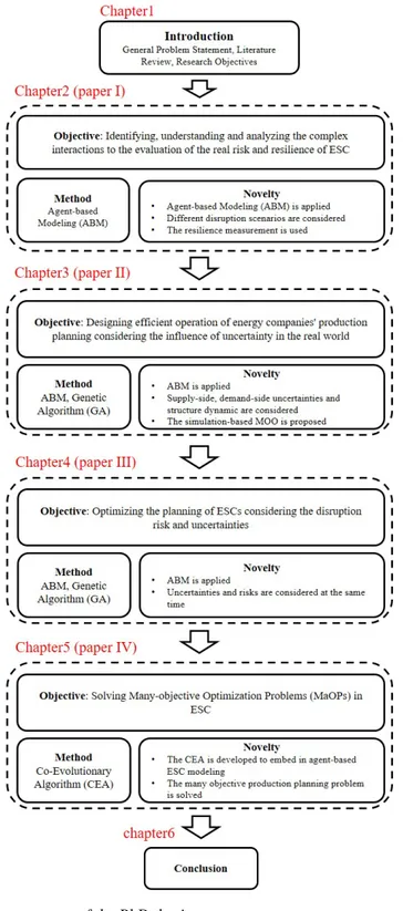
Thesis Structure

In Chapter 2, we develop an agent-based ESC to investigate the resilience of the whole ESC under different disruptions. Based on the agent-based ESC modeling in Chapter 2, the research in Chapter 3, Chapter 4, and Chapter 5 have been done. Chapter 3 consider a multi-objective optimization problem under the uncertainty and the structure dynamic in the ESC. In Chapter 4, besides the uncertainty and the structure dynamic, the disruption risk is considered when optimize the ESC. Also based on Chapter 3, a many-objective optimization problem is solved in Chapter 5. The related factors we consider are shown in Table 1.1.

Figure 1.3 shows the structure of this PhD thesis. The following 4 Chap-ters (from 2 to 5) are dedicated to the deepening of the theoretical back-ground of the exploited methods, to the description of the application and of the results provided by the developed methods, particularly focusing on the novelty and the original contributions introduced in this Ph.D. research work. Finally, in Chapter 6, some conclusions and remarks on the devel-oped work are drawn, and the perspective regarding the possible future ap-plications of the developed methods will be discussed. At the end of this Ph.D. thesis work, we also included a collection of the published/under re-view international journal papers to which the reader can refer to for further details.

(32)

(33)

SECTION II: DETAILS OF THE DEVELOPED

FRAMEWORK

This part is the main body of the thesis which includes 4 Chapters (from Chapter 2 to Chapter 5) and presents the original contributions of the re-search works.

(34)

(35)

CHAPTER

2

ABM for ESC Resilience Analysis

The objective of this work is to describe complex interaction between agents and assess the resilience of an ESC and for these we adopt an ABM frame-work, which allows modeling large interconnected systems. This capability comes from the fact that ABM is a bottom-up modeling approach, which focuses on modeling individual agents and their interactions, from which phenomena emerges, which are difficult to model by the traditional top-down modeling methods [43]. Every agent is defined by a set of behavioral functions, which give it intelligence to make decisions in response to its interactions with other agents and the environment. The simulation of the agents behaviours yields the overall system behavior.

2.1

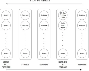
The Proposed Method

In this study, we take an oil supply chain as object of study. The supply chain is considered organized in five layers: retailers, bottling & storage, re-finery, port storage and crude oil producers. Every layer contains its agents, which are competitors. The structure of the ESC of the reference example is shown in Figure 2.1.

(36)

Figure 2.1: ESC structure

from the retailer (layer 1, on the right) to the producer (layer 5, on the left) in sequence, whereas the production, in turn, proceeds backward from the producers to the retailers. The basic idea of the negotiation strategy is that the demander sends orders to its preferred supplier. The supplier accepts or rejects the orders and, then, sends back its response. After a number of negotiation runs, the supply chain network sets up. The main parameters and variables are given below.

2.1.1 Modeling of agent uncertain behavior

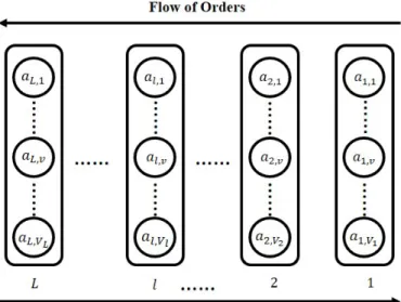
We consider an ESC with L layers and each l-th layer consists of Vlagents,

al,1, al,2, ..., al,v, ..., al,Vl (Figure 2.2). In the ESC, the orders sent from

Layer 1 flow layer-by-layer to the end layer L, whose VLagents are

suppli-ers that send supply decisions backward to the demandsuppli-ers.

An agent al,v, v = 1, 2, ..., Vl, in the l-th layer, is assigned with

behav-iors, which allow the agent to adaptively interact with the others. The de-tails of the model are described in the following.

2.1.1.1 Sending Orders

The process of sending orders of an agent al,vin the l-th layer (Figure 2.3)

is as follows:

(a) al,vchooses the supplier(s) al+1,v0 in the upper layer l + 1.

(b) al,vsends orders to al+1,v0.

(37)

2.1. The Proposed Method

Figure 2.2: The ABM-ESC model

(38)

2.1.1.2 Receiving Orders and Choosing Demanders

The process of an agent al,v receiving orders and choosing demander(s) is

shown in Figure 2.4 and described as follows:

(a) al,vreceives the order from al−1,v00 in the lower layer l − 1.

(b) al,vchecks whether the received order is empty:

• If yes, al,vdoes not choose demanders.

• Otherwise, (c) al,v checks whether it has available productions that

satisfy the received orders.

– If yes, (d) al,v checks whether the received orders exceed the

ex-isting production limitation Ul,v(t) defined as:

Ul,v(t) = Sl,v(t) − Sl,v∗ (t) (2.1)

where Sl,v is the storage of al,v and Sl,v∗ is the back-up safety

storage of al,v.

* If yes, (e) al,v refuses the order from al−1,v00 demanded with

the lowest bid price, and returns to (d).

* Otherwise, (f) the agent al,v accepts the order and makes a

contract with al−1,v00.

Then, the existing oil production limitation of the agent al,v

(Eq.(2.2)) updates for the next time t + 1: Ul,v(t + 1) = Ul,v(t) −

X

v00_,v00_∈{v a}

xl−1,v_l,v 00(t) (2.2)

where, xl−1,v_l,v 00(t) is the amount of orders accepted by the agent al,vwhich are sent by the agent al−1,v00

– Otherwise, (g) al,vsends a response back to the demander al−1,v00.

2.1.1.3 Response

One demander al,v may negotiate with its supplier al+1,v0, in case of

re-ceiving a response from al+1,v0. This process is shown in Figure 2.5 and

described as follows:

(a) The agent al,vreceives a response from the supplier al+1,v0.

(b) Check whether the order plan is satisfied: • If yes, al,vstops sending the order plan.

(39)

(40)

• Otherwise, (c) al,v checks whether all the alternative suppliers have

been considered:

– If yes, the agent al,vstops sending the order plan.

– Otherwise, (d) the agent al,v updates its demands,

yl+1,v_l,v 0(t + 1) = y_l,vl+1,v0(t) − X

v0_,v0_∈{v a}

xl,v_l+1,v0(t) (2.3)

where, y_l,vl+1,v0(t) is the amount of orders sent by the agent al,v

which are received by the agent al+1,v0 at time t, xl,v

l+1,v0(t) is the

amount of orders accepted by the agent al+1,v0 which are sent by

the agent al,v at time t.

And, (e) send orders (as discussed in Section 2.1.1.1) again.

2.1.1.4 Selling Production

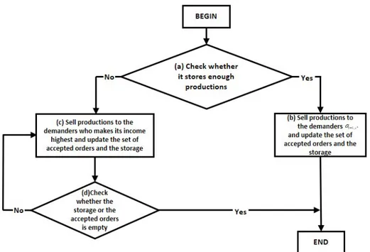
An agent al,v should sell productions after accepting an order plan. This

process is shown in Figure 2.6 and defined as follows:

(a) al,v checks whether it stores enough productions satisfying the

ac-cepted order plan:

• If yes, (b) sells the productions to the demander al−1,v00and updates the

set of accepted orders and the storage for the next time t+1 (Eq.(2.4)): Sl,v(t + 1) = Sl,v(t) −

X

v00_,v00_∈{v a}

z_l,vl−1,v00(t) (2.4)

where Sl,vis the production storage of al,vand, zl−1,v

00

l,v (t) is the amount

of the production sold by al,v to al−1,v00.

• Otherwise, (c) al,v sells the productions to the demander who makes

its income highest, and, then, updates the set of accepted orders and the storage Sl,v(t + 1).

(d) Check whether the storage or the set of accepted orders is empty. – If not, repeat (c).

(41)

(a) Receive a response from the

supplier (b) Check whether the order plan is satisfied (c) Check whether all the

suppliers have been considered? (d) Update

demands

(e) Another cycle of Sending Order END Yes Yes No No 1, 1, , , , 1, ,{} ( 1) ( ) ( ) a lv l v l v l v l v lv v vv y+¢t y+¢t x t ¢ + ¢ ¢Î + = -å BEGIN

Stop sending order

(42)

Figure 2.6: The process of selling production

2.1.1.5 Receiving Production

An agent al,v receives the oil production from the upstream agents al+1,v0

and updates its storage Sl,v(t + 1) for the next time t + 1:

Sl,v(t + 1) = Sl,v(t) + wl+1,v

0

l,v (t) · kl,v (2.5)

where Sl,v is the production storage of al,v, wl+1,v

0

l,v (t) is the amount of the

oil production sent by the the agent al,v which are received by the agent

al+1,v0 time t, k_l,v is the production capacity of a_l,v.

2.1.2 Resilience measurement

For simplicity, we consider a deterministic and static metric for measuring the resilience of the considered ESC ([79]), which is formally defined as:

RL = Z t2

t1

Q(t)dt (2.6)

where t1 and t2 are the endpoints of the time interval under consideration

(43)

2.2. Case Study

Figure 2.7: Resilience loss

Q(t) = 1 − V P i=1 D01,i(t) V P i=1 D1,i(t) (2.7)

where D is the quantity of the total production that customers demand and D01,i is the quantity of the total production delivered to the retailer after

disruptions. In words, Eq. 2.6 denotes the shaded area in Figure 2.7. To estimate the ESC resilience, we apply MC simulations. We repeat simulat-ing the ABM model for N times; in each trial, we insect a disruption and strategy. Then, we get resilience RLi(i = 1, 2, ..., N ). We finally average

the resilience values.

2.2

Case Study

According to the structure of the 5-layer ESC model, we assume that there are 5 agents in each layer. Every agent can implement the basic function like sending and receiving orders and production. The orders flow from the retailer agents to the producer agents, whereas the production flows from the producer agents to the retailer agents. In this case study, we consider several disruptions scenarios occurring in ESC. In order to investigate how these disruptions influence the resilience of the whole ESC, the following scenarios are considered.

Disruptions:

S1: an increase in demand (10%) for 15 transaction cycles S2: an increase in demand (30%) for 15 transaction cycles S3: a decrease in supply (10%) for 15 transaction cycles S4: a decrease in supply (30%) for 15 transaction cycles

(44)

Figure 2.8: The resilience loss in the scenario S1 and S2

S5: a break in supply process

In the scenario S5, we assume that if the disruption happens, agent a2,1in

Layer 2 cannot get oil production from upstream agents and thus, it cannot offer oil production for any downstream demanders.

To recover the ESC from disruption, we consider following strategies respectively: 1. The safety inventory. 2. The flexible production capacity. These strategies in detail are shown as follows.

Storage:

O1: Original storage

O2: Increasing storage 30% O3: Increasing storage 50%

Supplier:

A1: Increase internal production capacity by 5% of existing capacity A2: Increase internal production capacity by 10% of existing capacity

In each scenario, after the disruption happens, the retailers get less pro-duction than before, so there is a gap after the disruption happens which can be proven by comparing S1 and S2 in Figure 2.8 or S3 and S4 in Figure 2.9. However, if we take strategies, these strategies can effectively mitigate the influence of the disruption.

(45)

2.2. Case Study

Figure 2.9: The resilience loss in the scenario S3 and S4

(46)

If we take the safety inventory (O1, O2 or O3) in the retailer storage as the mitigatory strategy, we assume that once the disruption happens, the agents take actions immediately, so in the beginning, the resilience loss gets smaller. After a while, the safety inventory is depleted, so the resilience loss becomes same as the resilience loss without taking any strategies. The total resilience loss gets smaller if the safety inventory is larger which can be demonstrated by comparing S2O1, S2O2 and S3O3 in Figure 2.8, S4O1, S4O2 and S4O3 in Figure 2.9 and S5O1, S5O2 and S5O3 in Figure 2.10.

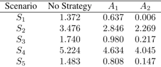
If we take the flexible production capacity (A1 or A2) in the finery as the mitigatory strategy, we still assume that once the disruption happens, the agents take actions immediately, but we increase the production capacity until the disruption terminates. The results show that increasing production capacity can effectively decrease the resilience loss which are demonstrated by comparing S2A1 and S2A2 in Figure 2.8, S4A1 and S4A2 in Figure 2.9 and S5A1 and S5A2 in Figure 2.10.

The resilience loss for disruption impact under different scenarios and recovery strategies are represented in Table 2.1 and Table 2.2 in detail.

Table 2.1: The resilience loss comparing with taking the safety inventory to mitigate the influence of disruption Scenario No Strategy O1 O2 O3 S1 1.372 1.126 1.044 0.990 S2 3.476 3.269 3.199 3.153 S3 1.740 1.473 1.383 1.323 S4 5.224 4.953 4.863 4.803 S5 1.483 1.302 1.242 1.202

Table 2.2: The resilience loss comparing with taking the flexible production capacity to mitigate the influence of disruption

Scenario No Strategy A1 A2 S1 1.372 0.637 0.006 S2 3.476 2.846 2.269 S3 1.740 0.980 0.217 S4 5.224 4.634 4.045 S5 1.483 0.808 0.147

In this work, we simulate a basic ESC model within the Agent-based simulation framework. The main agents in ESC as retailers, bottling & storages, refineries, port storages and crude oil producers, which can com-municate (sending and receiving orders) and interact (sending and receiving

(47)

2.2. Case Study

production) with each other. This ESC model is built for investigating the resilience of the whole ESC under different disruptions.

To this aim, we considered different scenarios and we used the resilience measurement to estimate the system resilience. It is notable that the more serious disruption will make more resilience loss. In addition, safety inven-tory and flexible production capacity are essential factors influencing the resilience of the ESC.

Based on this model, we know how disruption influence the resilience in the ESC. It also provides future scope for improvements. In the following, we plan to construct an Agent-based ESC model which has some specific difference from common supply chain and it is related to the energy system. How to design inter-system or/and inter-component dependencies and how to deal with their uncertainties will be more challenging. Finally, we desire to optimally design the ESCs with higher levels of resilience.

(48)

(49)

CHAPTER

3

A Simulation-based MOO Framework for

ESCs

Energy production companies have to make planning decisions to satisfy the customers uncertain demands and to maximize their own profits. In this work, we propose a simulation-based MOO framework for the efficient management of the ESC sustaining production. The ESC agents interaction is uncertain and the ESC structure can dynamically change. ABM is used to model and simulate the agents actions and behavior, and the ESC transac-tion processes. The simulatransac-tion is embedded into an NSGA-II optimizatransac-tion scheme for identifying the Pareto front of solutions for which the ESC total profit is maximized and the disequilibrium among the agents profits is mini-mized. Based on the Min-Max method, a single best compromised solution is identified. Finally, the MC simulations approach is used to operational-ize the proposed ABM-MOO framework in presence of the uncertainty that affects the ESC.

For demonstration, we consider an oil and gas ESC model with five layers, including crude oil producers, storages, refineries, terminal storages and retailers. The results show that the proposed framework enables the op-timization of the ESC planning, while taking into account multiple sources

(50)

of uncertainty and the structure dynamics that challenge the ESC operation.

3.1

The Planning Problem of The ESC

ESC can be effectively described by ABM. ABM can provide logical rules to describe the agent behavior and interactions and allows simulating the ESC transaction processes in an uncertain, dynamic and time-dependent environment [31, 45, 48, 80, 81]. Thus, in our work, we apply ABM to the modeling, analysis and optimization of ESCs, taking into account both the demand and supply uncertainties, and the structure dynamics.

We consider an ESC with L layers and each l-th layer consists of Vl

agents, al,1, al,2, ..., al,v, ..., al,Vl. In the ESC, the orders sent from Layer 1

flow layer-by-layer to the end layer L, whose VLagents are suppliers that

send supply decisions backward to the demanders.

An agent al,v, v = 1, 2, ..., Vl, in the l-th layer, is assigned with

behav-iors, which allow the agent to adaptively interact with the others. The de-tails of the model are described in Chapter 2 Section 2.1.1.

In the aforementioned ESC, each agent al,vneeds to make decisions on

the planning to satisfy its customers uncertain demands and to maximize the own profits. This is challenging due to the fact that the uncertainty originating from the production and purchase quantities (e.g., cost, price, demand, supply, etc.) influences the agents decisions associated with the interaction structure, which, in turn, affects the agents profits. The uncer-tainty propagates throughout the dynamic transaction process in the whole ESC, making it difficult to deal with production schedules and purchase orders.

To deal with this, we formulate a MOO problem in terms of the ESC total profit (that is expected to be maximized) and the agents own profits (for which the disequilibriums are supposed to be minimized).

Eq.(3.1) defines the ESC total profit P :

P = T X t=1 L X l=1 Vl X v=1 (A − B − C) − D (3.1)

where A is related to the income from selling the oil production to the customer, expressed in Eq.(3.2).

A =

V_l−100

X

v00₌₁

(51)

3.1. The Planning Problem of The ESC

where pl−1,v_l,v 00is the unit price of the agent al,vwhen selling the oil

produc-tion to the agent al−1,v00, zl−1,v 00

l,v (t) is the production sent by the agent al,v,

which is received by the agent al−1,v00 at time t.

B is the purchase cost, which includes the procurement cost plus the other costs e.g. the transportation cost, the labor cost and so forth.

B = V0 X v0₌₁ (pl,v_l+1,v0 + o l+1,v0 l,v )w l+1,v0 l,v, (t) (3.3)

where pl,v_l+1,v0 is the unit price of the agent a_l+1,v0 for selling the oil

produc-tion to agent al,v , ol+1,v

0

l,v is the unit price for the other cost, w l+1,v0 l,v,t is the

amount of the oil production sent by the agent al+1,v0, which is received by

the agent al,v.

The item C calculates the storage cost.

C = cS_l,vSl,v(t) (3.4)

where cS_l,v is the agent al,v storage unit cost, Sl,v,t is the production storage

of the agent al,v at time t.

And, D is a penalty from the loss [82], D =

T

X

t=1

r(t)εP (3.5)

where r(t) is equal to 1 when the agent suffers a loss after the oil production transaction at time t; otherwise, 0. εP is an arbitrary large number for the

total profit.

On the other hand, the profits of the agents are expected to be different in a healthy ESC. It is of importance to measure and control the disequi-libriums among the agents own profits, E, which is defined as the sum of the dispersion quantifying the deviation of the agents real profits from the expected values (F ) and the penalty of loss in all the transaction cycles (G):

E = F + G (3.6) F = L X l=1 σ_l2 |µl| (3.7) G = T X t=1 r(t)εE (3.8)

(52)

where σl is the standard deviation of the profits of the agents in the layer

l, µlis the mean of the agents profits in the layer l, r(t) is equal to 1 if the

agent suffers a loss after the oil production transaction at time t; otherwise, 0. εE is an arbitrary large number for the disequilibrium.

Hence, the MOO problem can be formulated: max P (¯y1,1, ..., ¯yl,v, ..., ¯yL−1,VL, p 1,1 2,1, ..., p l−1,v00 l,v , ..., p L−1,VL−1 L,VL ) (3.9) min E(¯y1,1, ..., ¯yl,v, ..., ¯yL−1,VL, p 1,1 2,1, ..., p l−1,v00 l,v , ..., p L−1,VL−1 L,VL ) (3.10) s.t. ¯ ymin_l ≤ ¯yl,v≤ ¯ymaxl (3.11) pmin_l ≤ pl−1,v_l,v 00 ≤ pmax l (3.12)

The problem will be solved by maximizing the ESC total profit (3.9) and minimizing the disequilibrium (3.10), simultaneously. Eq.(3.11) and Eq.(3.12) are constraints defining the feasible regions for the average orders and the prices.

3.2

The ABM-MOO Framework

An ABM-MOO framework is originally proposed to obtain the non-dominant solutions of the Pareto fronts, which can maximize the total ESC profit P and minimize the disequilibrium among the agents profits E. To account for demand and supply uncertainties, MC simulations are used, as sketched in Figure 3.1, to operationalize the ABM-MOO framework. NSGA-II as a type of GA is easy and flexible to be applied to the optimization problem in our ESC. The general advantages of NSGA-II are list as follows [83]: 1. The non-dominated sorting techniques is used to get the optimal solution closely. 2. The crowding distance techniques is used to maintain diversity of the solutions. 3. The elitist techniques is used to preserve the best solu-tion in the next generasolu-tion. Specially, in our case, the number of decision variables is 39 which is difficult to be solved by derivative based methods but can be easily encoded and then optimized by NSGA-II.

The algorithm is summarized as follows: Initialization

• Initialize the MC simulations.

(53)

3.2. The ABM-MOO Framework

Initialization of the ABM-MOO in each n-th MC run

• Set the transaction time t = 0, 1, 2, ..., N Tmax, the GA population size

N P , the maximum number of GA generations N Gmax, the crossover

coefficient Ccand the mutation coefficient Mc.

• Generate QL,VL(t) ∼ N (µQ, σ

2

Q), where QL,VL(t) is the amount of

productions which are produced by the agent aL,VL in the last layer at

time t, µQis the average value, σ2Qis the variance.

• Set the NSGA-II generation index k = 1.

• Randomly generate the order and price decision matrices P OPn i (k) = {[¯y1,1, ..., ¯yl,v, ..., ¯yL−1,VL, p 1,1 2,1, ..., p l−1,v00 l,v , ..., p L−1,VL−1 L,VL ] n 1, ..., [¯y1,1, ..., ¯yl,v, ..., ¯ yL−1,VL, p 1,1 2,1, ..., p l−1,v00 l,v , ..., p L−1,VL−1 L,VL ] n

N P} within the feasible space. They

are coded into the chromosomes of the GA. • Generate y_l,vl+1,v0(t) ∼ N (¯yl,v, σ2y), where y

l+1,v0

l,v (t) is the amount of

orders sent by the agent al,v which are received by the agent al+1,v0 at

time t, ¯yl,vis the average value and σ2y the variance.

Begin the NSGA-II loop

• Input all the generated values into the ABM ESC model, to simulate the transactions.

• Calculate the values of P and E, according to Eq.(3.1) and Eq.(3.6), respectively.

• Rank the chromosomes P OP_in(k) by running the fast non-dominated sorting algorithm.

• Rank the chromosome P OP_in(k) based on the crowding distance, aimed at finding the Euclidean distance between chromosomes in a front that maximizing P and minimizing E. It is worth pointing out that the chromosomes in the boundary are selected all the time, since they are assigned with infinite distance.

• Select the chromosome P OPn

i0(k) by using a binary tournament

selec-tion with crowded-comparison-operator(≺λ), where λ is a predefined

tournament size.

• Apply the polynomial mutation [84, 85] and the simulated binary crossover operator [84, 86] to generate the offspring populations P OP_in (k + 1).

(54)

• Set k = k + 1 and check that the NSGA-II stopping criterion (k > N Gmax) is reached:

– If yes, return the ranked Pareto-optimal {F₁n, F₂n, ..., F_ndn} where F₁nis the best front and F_ndn is the least good front, set n = n + 1. – Otherwise, begin a new NSGA-II cycle.

• Check whether the MC simulations stopping criterion reaches (n > M Gmax).

– If yes, end ABM-MOO and get all the Pareto fronts. – Otherwise, begin a new MC simulations cycle.

Notice that a set of Pareto fronts can be identified from each MC run of the ABM-MOO framework and a best compromised solution can be identified among them by the Min-Max method [87, 88]. The Min-Max finds the highest value that one objective can be sure to get without know-ing the strategy that would satisfy the other objective. Given Pareto front H ≡ (P, E) the relative deviations of P and E are defined, respectively:

zP =

|P − Pmin_|

Pmax_{− P}min (3.13)

where Pmin_{and P}max_{are the minimum and maximum of the fitness values}

P , respectively.

zE =

|E − Emin_|

Emax_{− E}min (3.14)

where Emin_{and E}max_{are the minimum and maximum of the fitness values}

E, respectively.

The best compromised solution is determined as

zH = min[max{zP, zE}] (3.15)

3.3

Case Study

For illustration, we consider an oil ESC which is structured in five layers, including retailers (Layer 1), terminal storage (Layer 2), refinery (Layer 3), storage (Layer 4) and crude oil producers (Layer 5). Three cooper-ative agents are modeled in Layer 1 (i.e., a1,1, a1,2, a1,3), Layer 2 (i.e.,

(55)

3.3. Case Study

(56)

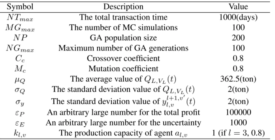
Table 3.1: The setting of the parameters for the ABM-MOO

Symbol Description Value

N Tmax The total transaction time 1000(days)

M Gmax The number of MC simulations 100

N P GA population size 200

N Gmax Maximum number of GA generations 100

Cc Crossover coefficient 0.8

Mc Mutation coefficient 0.8

µQ The average value of QL,VL(t) 362.5(ton)

σQ The standard deviation value of QL,VL(t) 2(ton)

σy The standard deviation value of yl+1,v

0

l,v (t) 2(ton)

εP An arbitrary large number for the total profit 100000

εE An arbitrary large number for the uncertainty 1000

kl,v The production capacity of agent al,v 1 (if l = 3, 0.8)

Table 3.2: The values of the orders and prices limitations

l = 1 l = 2 l = 3 l = 4 ¯ ymin l (ton) 100 100 100 100 ¯ ymax l (ton) 400 450 300 600 pmin_l (¤/ton) 40 25 15 10 pmax_l (¤/ton) 55 40 25 15

are modeled in Layer 4 (i.e., a4,1, a4,2) and Layer 5 (i.e., a5,1, a5,2),

respec-tively.

Customer agents try to get enough productions from suppliers and, at the same time, supplier agents have to choose the demander(s) who can bring them the highest profits. Motivated by this, agents take relative behaviors to realize their expectations. These behaviors have been illustrated in Chapter 2 Section 2.1.1, and define the rules and decision processes of the agents interacting with other agents in an uncertain environment.

We apply the ABM-MOO framework to the ABM of the aforementioned oil ESC, for a total of M Gmax = 100 MC simulations runs, in a period of

1000 transaction days. Table 3.1 summarizes the main parameters set for the ABM-MOO algorithm. Table 3.2 lists the constraints as discussed in Eqs.3.11 and 3.12, and Table 3.3 lists the unit prices ol+1,v_l,v 0 for the other cost from al+1,v0 to a_l,v. The uncertain variables are distributed as Gaussian