ALMA MATER STUDIORUM - UNIVERSITÀ DI BOLOGNA
FACOLTA’ DI INGEGNERIA
CORSO DI LAUREA IN INGEGNERIA CIVILE
Dipartimento di Ingegneria delle strutture.
dei Trasporti, delle Acque, del Rilevamento, del Territorio (D.I.S.T.A.R.T.)
TESI DI LAUREA
in
Calcolo Automatico delle Strutture
Monitoraggio delle condizioni strutturali
del Rio Dell – Hwy 101/Painter Street Overpass
attraverso l’utilizzo di dati dinamici
CANDIDATO: RELATORE:
Luciana Balsamo Prof. Francesco Ubertini
CORRELATORE: Prof. Raimondo Betti
Anno Accademico 2008/2009 Sessione III
Computers are incredibly fast, accurate and stupid. Human beings are incredibly slow,
inaccurate and brilliant. Together they are powerful beyond imagination.
Table of Contents
1. INTRODUCTION
Pag. 1
2. REVIEW OF PREVIOUS STUDIES
Pag. 8
2.1 Introduction
Pag. 9
2.2 The Geometrical Characteristics of the Bridge
Pag. 10
2.3 Dynamic Characteristics of the Bridge
Pag. 11
2.4 Soil-Structure Interaction
Pag. 26
2.5 Structural Identification through OKID
Pag. 32
3. SYSTEM IDENTIFICATION VIA OKID/ERA
Pag. 34
3.1 Introduction
Pag. 35
3.1.1 The Historical Path of OKID/ERA Algorithm Pag. 37
3.2 Basic Formulation
Pag. 38
3.2.1 Input-Output Relations Pag .37
3.2.2 Observer/Kalman filter IDentification Pag. 41
3.2.3 Eigensystem Realization Algorithm Pag. 43
3.2.4 Refining the Identified State-Space Model Pag. 45
3.2.5 Recovering the Dynamics of the System from the
Realized State-Space Model
3.3 Numerical Results
Pag. 51
3.3.1 Trinidad Offshore (November 8, 1980) Pag. 54
3.3.1.1 Discussion of the Results Pag. 57
3.3.2 Rio Dell Earthquake: Discussion of the Results Pag. 72
3.3.3 Petrolia Earthquake: Discussion of the Results Pag. 86
4. FINITE ELEMENT MODEL
Pag. 100
4.1 Introduction
Pag. 101
4.2 Formulation of the Displacement-Based
Finite Element Method
Pag. 103
4.2.1 General Derivation of Finite
Element Equilibrium Equations
Pag. 105
4.2.1.1 The Principle of Virtual Displacements Pag. 107
4.2.1.2 Finite Element Equations Pag. 109
4.2.2 Finite Element Formulation for Euler Beams Pag. 112
4.2.3 Finite Element Formulation for Plates and Shells Pag. 115
4.2.3.1 Kirchhoff Plate Pag. 116
4.2.4 Modal Analysis Pag. 120
4.2.4.1 Verification Example: Modal Analysis
of a Beam via STRAUS7 and SAP2000
Pag. 122
4.3 Finite Element Models
Pag. 125
4.3.1 First Model: the Beam Model Pag. 125
4.3.2 Second Model: the Grid Model Pag. 129
4.3.3 Third Model: Shell Model Pag. 142
4.3.3.1 The Shell Element in SAP2000 Pag. 142
4.3.3.2 Thick-Shell Elements Model Pag. 145
4.3.3.3 Thin-Shell Elements Model Pag.149
4.4 Model Calibration
Pag. 155
4.4.1 Genetic Algorithm (GA) Pag. 155
4.4.2 The Code Used in the Optimization Process Pag. 157
4.4.2.1 Tournament Selection with
a Shifting Technique
Pag. 159
4.4.2.2 Single Point and Uniform Crossover Pag. 159
4.4.2.3 Jump and Creep Mutation Pag. 160
5. CONCLUSIONS
Pag. 161
BIBLIOGRAPHY
Pag. 164
1
1
INTRODUCTION
Sommario
Il problema del monitoraggio delle condizioni strutturali di sistemi quali quelli pontuali è divenuto ormai un tema centrale nel campo dell’ingegneria civile. Per questo, negli ultimi decenni, si sono sviluppati sempre più metodi aventi come obiettivo quello del controllo dello stato della struttura. Molto sviluppati, in questo senso, sono quelli che si avvalgono di dati dinamici, registrati ad esempio da strumenti quali gli accelerometri. Questi metodi permettono l’osservazione dello stato strutturale del sistema oggetto d’analisi e nel contempo possono fornire informazioni utili per il rinvenimento di danno, generatosi, ad esempio, a seguito di un evento sismico importante. Nel presente lavoro è stata compiuta l’analisi strutturale del Rio Dell – Hwy 101/Painter Street Overpass.
Il Painter Street Overpass è collocato presso Rio Dell, nella California del Nord (Figure 1.1). Si tratta di un ponte a due campate, con impalcato a cassone in cemento armato precompresso. La geometria è complicata da un’inclinazione pari a 38.9 gradi dell’asse trasversale dell’impalcato rispetto a quello longitudinale. Il ponte è stato munito di accelerometri nel 1977 ad opera del Dipartimento dei Sottosuoli e della Geologia della California. In figura 1.2 è mostrata la disposizione di tali strumenti.
Il metodo di monitoraggio qui proposto si sviluppa in cinque passaggi. Essenzialmente, la vera e propria fase di monitoraggio si esplica solo al quinto passo, mentre i primi quattro possono considerarsi stadi necessari alla creazione di strumenti indispensabili per la finale individuazione del danno.
2
The use of dynamic data aimed to structurally identify systems such as bridges has become a well known non-destructive method able to provide evaluation of the condition of the structure. The subject of the present work is the Rio Dell - Highway 101/Painter Street Overpass, California. The approach presented herein is thought to offer an almost immediate estimation of whether or not the bridge under consideration has suffered some damage and, possibly, the location of the damage.
The Painter Street Overpass is located near Rio Dell, in Northern California (Figure 1.1). It is a continuous, two span, cast-in-place, pre-stressed post-tension, concrete, box-girder bridge. The geometry is complicated by a 38.9 degrees skew of the bent with respect to the deck longitudinal axis. The bridge was instrumented in 1977 by the California Division of Mines and Geology. Figure 1.2 shows the location of the accelerometers.
The health condition monitoring method here proposed is developed in five stages. Essentially, the proper monitoring phase is only the fifth one, while the first four can be considered as the necessary steps that have to be taken in order to create the indispensable tools required for the final damage detection.
3
First Phase: Review of Previous Studies
The review of previous studies enables to have some granted information on the structure, resulting as a starting point for the development of the actual work. At this stage, one should not seek any detail in particular. Any data gained should be accurately analyzed, since they could offer some hints such as indications on how to model the system, or suggestions on the boundary conditions to employ.
Second Phase: Structural Identification through OKID Algorithm
In this part, special attention is devoted in identifying the dynamic characteristics of the bridge. An Observer/Kalman filter Identification (OKID) algorithm is applied using the recorded time histories available at the Center of Engineering Strong Motion Data website. This stage is essential to define the modal characteristics that will be some of the thresholds of the calibration of the mechanical model that will be built in the following step.
Third Phase: Linear Finite Element Model of the Bridge
It consists in developing a linear finite element model of the bridge.
This part is crucial in the development of the future steps. It is required to the finite element model to be the most accurate as possible, in order to constitute a reliable tool on which perform the future damage detection. A number of finite element models are created with an increasing level of detail. Once the modal characteristics and the response of the model cannot be improved any further, the model has to be calibrated. In this study a genetic algorithm is applied. The calibration thresholds are the modal frequencies identified in the previous step, and the acceleration time histories available for the Painter Street Overpass.
4
Fourth Phase: Non-Linear Finite Element Model
The previously generated FE model is extended to the nonlinear range. By progressively increasing the load in the three space directions, the most stressed zones of the system are individuated. In these areas the elastic limit can be overcome, but this may not necessarily imply damage is occurred. On the contrary, it may only mean that the system has a non-linear behavior. Therefore, introducing non-linear elements in the most stressed regions will lead to handle with a model that will resemble more likely the actual response of the bridge. The simulated time histories of the response from the nonlinear model represent a new set of data that are used in the next phase to test rapid response evaluation tools.
Fifth Phase: Damage Detection
This phase is herein presented to utterly describe the approach. Nonetheless, the phase explained below has not been tested, since the Painter Street Overpass had not suffered any damage at the time of the research.
The “amplified” ground motion time histories are fed through the high-fidelity bridge model developed, and the predicted response of the bridge at the various sensor locations on the superstructure is estimated. If the predicted response of the model matches the simulated response from Phase IV at all of the sensor locations, it will be indication that no damage has occurred in the bridge. If, instead, the previously identified model provides structural responses that do not match the ones from Phase IV, then this will serve as a caution that damage might have occurred somewhere in the bridge. Since the nonlinear response data are simulated through the model developed in Phase IV, different damage levels will be investigated and a sensitivity analysis on the damage intensity level should be performed.
Another indicator of potential damage could consist in the relative displacements between critical sensor locations. Using the nonlinear model from Phase IV, time histories of the structural displacements at different sensor
5
locations and their relative magnitude will be determined. A displacement between two recording stations that is close to or beyond a certain threshold will be an indication of potential damage between the two sensor locations and an in-depth damage assessment at that specified location will be necessary. This indicator can also be obtained in a relatively short time after the occurrence of the earthquake and can be run concurrently at the first approach.
6
7
8
2
REVIEW OF PREVIOUS STUDIES
Sommario
Il capitolo che segue è frutto della ricerca bibliografica di studi precedentemente compiuti, aventi come oggetto il Rio Dell Overpass. Una volta reperito la maggior quantità di materiale possibile sull’argomento, è possibile analizzarlo e cogliere spunti di approfondimento. In particolare, nel seguito verranno analizzate le caratteristiche geometriche della struttura, il comportamento dinamico desunto dai dati ambientali registrati dagli accelerometri di cui il ponte è stato munito dal 1977 ad opera del Dipartimento dei Sottosuoli e della Geologia della California, l’interazione terreno-struttura ed infine verrà introdotto il problema dell’identificazione strutturale per mezzo dell’algoritmo OKID/ERA, sebbene nella letteratura scientifica sia difficile trovare pubblicazioni a rigurado. Infatti, l’algoritmo menzionato è stato creato per applicazioni nel campo dell’ingegneria aeronautica e solo ultimamente è stato introdotto nel campo dell’ingegneria civile.
9
2.1 Introduction
As mentioned in the previous chapter, the Rio Dell Overpass was instrumented in 1977 by the California Division of Mines and Geology with twenty accelerometers (Figure 1.2). Eighteen accelerometers were located on the north edge of the bridge, while the remaining three sensors were put on the embankment in order to measure free field accelerations. However, the position of the channels give some problems for the determination of the characteristics of the system. Since the bent is skewed, the deck torsional deformations are not negligible. Nonetheless, the torsional contribute to the deformation cannot be caught only by means of the consideration of the recorded accelerations. It results apparent the necessity of the finite element model for a detailed structural identification of the Rio Dell Overpass.
Moreover, despite the fact that the bridge was instrumented thirty three years ago, accelerograms of only three earthquake events are available at the Center of Engineering Strong Motion Data (CESMD) website. Therefore, maybe these are some of the reasons why there are not many papers published on the Painter Street Overpass subject. Nevertheless, the researches available offer very helpful hints for structural identification through both OKID algorithm and finite elements model.
Essentially, the literature available on the subject of the Painter Street Overpass is focused on the characteristics of the bridge derived from the acceleration time histories analysis. The soil-structure interaction is another issue accurately described in many papers.
The literature on the use of the OKID/ERA algorithm for the structural identification is less ordinary. In fact, this is one of the first research in which this tool is exploited for structural purposes. The OKID/ERA algorithm was born in the mechanical engineering field, and only recently, for an intuition of Professor Betti and Professor Longman, has begun to be successfully tested in the civil engineering field.
10
2.2 The Geometrical Characteristics
of the Bridge
Identified as CSMIP Station No. 89324, the US 101/ Painter Street Overpass is located in Rio Dell, California. The Rio Dell overpass is a two span bridge crossing Highway 101 at Painter Street, 265 feet long. The bridge is a monolithic, cast in place, prestressed concrete, multi-cell box girder road deck with end diaphragm abutments and a two columns bent. Both the abutment and bent foundations are supported on piles. The behavior is complicated by a 38.9 degrees skew between the centerline of the bent and the centerline of Highway 101 passing. The bent spans 38 feet measured along the centerline of the skewed cross sections and is monolithically connected top and bottom to the footings and superstructure respectively. The columns are approximately 20 feet in height. The abutments have been constructed on top fill material to provide appropriate vertical clearance over Highway 101 below. The west abutment rests on a neoprene bearing strip which is part of a designed thermal expansion joint. All of the foundations are supported on driven 45 ton concrete friction piles.
11
2.3 Dynamic Characteristics of the Bridge
Due to the records of the seismic events that interested the bridge since the Trinidad Earthquake in 1980, it is possible to examine the dynamic behavior of the bridge by means of the analysis of the aforementioned records. The following analysis are inspired by some papers published by Prof. Romstad, from the California University.
The first analysis performed consists in calculating and plotting the power spectral density functions for individual earthquakes for each sensor. Figures 2.1 show the results. From the observation of all figures 2.1, it can be inferred that earthquakes tend to show a spike at 3.3 – 3.6 Hz, indicating an active natural mode with significant participation of all of the sensors. Other spikes tend to be concentrated at about 2.3, 4.2-4.4, 5.5 and 6.8 Hz. Nonetheless, only figures 2.1b and 2.1c show clearly dominating spikes; in particular, for sensor 6 two natural frequencies can be identified at 3.37 and 5.45 Hz, while for sensor 8 the dominating frequencies correspond to the values of 3.42, 4.40 and 6.98 Hz. However, it should be important to analyze the contribute to the modal characteristics of sensors 9 and 11, since they are the only sensors that measure transversal and longitudinal accelerations respectively. Anyway, observation of figures 2.1d and 2.1f demonstrates that the measurements recorded from these channels are quite invalidated by the noise. Therefore, only the modal frequencies at 3.42-3.52 Hz and at 4.20 Hz can be considered reasonable, since the frequency content of the other channels show this values too. Summarizing, from this initial analysis, four modal frequencies can be identified: the first is in the range from 3.2 to 3.6 Hz, and is supposed to have both longitudinal and vertical and transverse contributes, since all of the channels have a peak corresponding to this value; then, the modal frequency of about 4.3 Hz is identified by both vertical and transverse channels; follow the modal frequencies at 5.5 and 7 Hz, both identified through sensors that measure vertical accelerations.
12
13
14
15
16
17
18
Another analysis is performed on the Fourier transforms of the time histories recorded from channels that measure accelerations at the base of the pier (1, 2, 3), in free field (12, 13, 14), at the top of the east abutment (15, 16, 17) and on the bridge deck above the same abutment (9, 10, 11). First of all, the average value of the records between the Trinidad and Petrolia earthquakes is computed. Then, the Fourier transforms of the resulting time histories are calculated, grouping the plots depending on the direction of the measured motions. Then, three plots are obtained: the first representing the frequency content of the longitudinal accelerations, from channels 1, 11, 12 and 15; the second presenting the vertical accelerations, from sensors 2, 10, 13 and 16; the last showing the transverse behavior, from accelerometers 3, 9, 14 and 17. Results are presented in figures 2.2.
Analysis of figures 2.2 demonstrates a minor soil-structure interaction in the area of the pier. In fact, free field and base of the pier motions are similar. On the other hand, the interaction soil-structure is considerable in the area of the embankment, as can be inferred from the differences between the free filed and the top of abutment motion. Lastly, the similarity of the motions on top of the fill with the motions on the bridge deck could imply that the embankment fill moves with the bridge deck.
The trend identified via Fourier Transforms is found again by comparing the acceleration amplitude of the channels, plotted in figures 2.3. The maximum longitudinal accelerations on the abutment fill and on the structure are essentially the same as the free field motion for all earthquakes, possibly indicating the bridge is moving as a rigid body with the ground in the longitudinal direction. Practically, the same behavior is observed in the vertical direction. On the contrary, in the transverse direction the abutment and deck accelerations are amplified compared to the free field ones.
These observations offer valuable information on how to model the boundary conditions of the finite element system. In fact, the soil-structure interaction between the base of the pier and the soil can be modeled through fixed
19
restraints, since the two systems move together as a rigid body. On the other hand, the area through which the deck approaches the abutment does not need any special representation, for the two systems move as rigid body as well. On the contrary, the soil-structure interaction needs to be well understood and then modeled at the abutment level. As will be deeply clarified in the following paragraph, the best model for this connection is represented by a set of springs, whose stiffness choice constitutes a crucial step to obtain a model with realistic response.
Other interesting information on the dynamic behavior of skewed bridges can be found in a paper of Eng. Shamsabadi and Eng. Kapuskar. The research of the two engineers is focused on the determination of the response of skewed bridges to seismic inputs as a function of skew angle. Their results have obtained by exciting three-dimensional model of two-span box girder bridges with a skew angle varying from 0 to 60 degrees with non-linear time histories. It is observed that skewed bridges are affected by strong rotations with respect to the vertical axis during the seismic event, while present an irreversible transverse displacement after the shaking is terminated. On the contrary, the bridge with zero skew angle do not show this behavior. Moreover it is observed that, for particularly intense ground motions, the deck could experience the unseat at the abutments. The engineers clarify that what causes the severe deck rotations is a non uniform passive soil wedge behind the abutment wall, that results in asymmetric soil reactions of the wall itself. What deserves to be underlined is that the response changes as the direction of the applied motions vary. Therefore, it is important to be provided of earthquake time histories with more than one component and different records in order to completely identify the dynamic behavior of a skewed bridge.
20 0 5 10 15 20 25 30 0 0.1 0.2 0.3 0.4 0.5 0.6 0.7 0.8 0.9 1
Fourier Transform (Longitudinal Motion)
frequency (Hz) N o rm a lize d A m p lit u d e Pier Base Deck Free Field Abutment
21 0 5 10 15 20 25 30 0 0.1 0.2 0.3 0.4 0.5 0.6 0.7 0.8 0.9 1
Fourier Transform (Vetical Motion)
frequency (Hz) N o rm a lize d A m p lit u d e Pier Base Deck Free Field Abutment
22 0 5 10 15 20 25 30 0 0.1 0.2 0.3 0.4 0.5 0.6
Fourier Transform (Transverse Motion)
frequency (Hz) N o rm a lize d A m p lit u d e Pier Base Deck Free Field Abutment
23 5 5.5 6 6.5 7 7.5 8 8.5 9 9.5 10 -200 -150 -100 -50 0 50 100 150
Time Histories of Longitudinal Motions (channels 11, 12 and 15)
Time [sec] A cce le ra ti o n [ cm /se c 2 ] Deck Free Field Abutment
24 5 5.5 6 6.5 7 7.5 8 8.5 9 9.5 10 -100 -50 0 50 100 150
Time Histories of Vertical Motions (channels 10, 13 and 16)
Time [sec] A cce le ra tio n [ cm /se c 2 ] Deck Free Field Abutment
25 5 5.5 6 6.5 7 7.5 8 8.5 9 9.5 10 -300 -200 -100 0 100 200 300
Time Histories of Transverse Motions (channels 9, 14 and 17)
Time [sec] A cce le ra tio n [ cm /se c 2 ] Deck Free Field Abutment
26
2.4 Soil-Structure Interaction
As derived in the previous paragraph, it is essential to individuate a model through which reasonably represent the soil-structure interaction at the base of the abutment. Moreover, the final aim of this study is obtaining a realistic non-linear model of the Rio Dell Painter Street Overpass. It becomes apparent that this leads to deal with large displacements theory. As displacements raise, the behavior of bridge abutments cannot be modeled as linear anymore. Studies proved that the peak accelerations recorded near and on highway overcrossing approach embankments can be more than twice the crest motion of the pile cap of the center bent. Then, the kinematic response of the embankment strongly effects the bridge response. Design procedures used by Caltrans (1989) solve the problem by means of distributed linear springs whose objective is modeling the stiffness of the embankment. Nevertheless, the Caltrans approach does not take into account neither the energy absorbed by the embankment nor the dynamic nature of the problem. Thus, this simplified approach becomes unacceptable when there is an attempt to seek more detailed results.
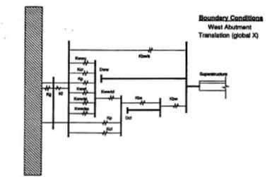
The solution proposed by Prof. Romstad consists of a complex system of springs reflecting soil, pile, concrete and interaction properties, as the one presented in figure 2.4. At both abutments the wingwalls are pinned with respect to moment about the vertical global Y axis. The wing wall cannot move out from the centerline of the bridge, once the joint filler is crushed to transfer the load. Nevertheless, there is not resistance to movement of the wingwall toward the longitudinal centerline of the bridge, except frictional resistance at the base of the wingwall. Moreover, the west backwall and the foundation are separated by a ¼” neoprene bearing strip. Shear keys bound the abutment backwall in the case gross relative displacements in both transverse directions and in the skewed longitudinal direction such that the backwall cannot move into the soil.
27
Figure 2.4a: Elevation View of Longitudinal West Abutment Resisting Elements
Figure 2.4b: Schematic Representation of Longitudinal West Abutment Active Spring Elements
However, this model seems to be very complex to apply and to be implemented in an FE model. Therefore, it is looked for another model. The research published by Zhang and Makris seems to achieve the purpose. The two researchers presented a study on Painter Street Overpass, providing the values of
28
the spring stiffness and dash-pot damping coefficients that can be used in a three dimensional finite element model in order to represent the soil-structure interaction at the end abutments. In the first phase of the method, the kinematic response of the embankments is evaluated. Through this step the shear modulus G and the damping coefficient of the soil embankment are determined. In particular, the shear modulus of the Rio Dell Overpass embankment is set equal to 8 MPa, while the damping coefficient equals 0.5. Then, it is possible to complete the dynamic stiffness calculation. Since this second phase is the one that leads to the values of interest, the detailed calculations are presented below:
1. Computation of the dynamic stiffness of the unit-width shear wedge:
) kz ( Y H z k J ) kz ( J H z k Y ) kz ( Y H z k J H z k Y ) kz ( J k B i 1 G ) ( kˆ 0 0 0 0 0 0 0 0 0 1 0 0 0 0 0 1 c x (2.1) where G = 8 MPa = 0.5 Vs = 190 m/s Bc = 15.24 m z0 = 3.81 m H = 9.6 m k = ) i 1 ( Vs J0() = Zero Order Bessel Function of the First Kind
J1() = First Order Bessel Function of the First Kind
Y0() = Zero Order Bessel Function of the Second Kind
29
2. Plot of the real and the imaginary parts of equation 2.1 as a function of frequency f = /2: 0 2 4 6 8 10 12 14 16 18 20 5 10 15 20 25 30
Real Part of Dynamic Stiffness of the Unit-Width Shear Wedge
frequency [Hz] k x [ M N /m 2 ]
Figure 2.5: Plot of the Real Part of Equation 2.1
0 2 4 6 8 10 12 14 16 18 20 0 50 100 150 200 250
Imaginary Part of Dynamic Stiffness of the Unit-Width Shear Wedge
frequency [Hz] k x [ M N /m 2 ]
30
3. Selection of practical spring and dash-pot values by passing a horizontal line through the graph of the real part and inclined line through the graph of the imaginary part at locations that capture with satisfaction the low frequency behavior: 0 2 4 6 8 10 12 14 16 18 20 5 10 15 20 25 30
Practical Spring Value
frequency [Hz] k x [ M N /m 2 ]
Real Part of Equation 1 Practical Spring Value
Figure 2.7: Practical Spring Value
0 2 4 6 8 10 12 14 16 18 20 0 50 100 150 200 250
Practical Dash-Pot Value
frequency [Hz] k x [ M N /m 2 ]
Imaginary Part of Equation 1 Practical Dash-Pot Value
31
Figures above show that the practical spring value can be taken equal to 25.413 MN/m2, while the slope of the imaginary part of the unit-width shear wedge gives the practical dash-pot value of the soil embankment:
=10.992 (2.2)
4. Computation of the transverse spring and dash-pot values of the embankment by multiplying the practical values with the critical length defined by equation 2.3: 987 . 5 H B S 7 . 0 Lc c (2.3) where S = 0.5 Bc = 15.24 m H = 9.6 m
Finally, the transverse and longitudinal values of the spring stiffness are:
ft / lbf 450 , 425 , 10 m / MN 148 . 152 k kx y (2.4)
while the transverse and longitudinal values of the dash-pot damping coefficients are: 809 . 65 y x (2.5)
32
2.5 Structural Identification through OKID
Examination of the literature demonstrates that essentially the subject is explored in the damage identification field. The most common use of the OKID tool is that where data is recorded at two different period of time, and the goal is that of establish whether the system has suffered damage in the time between the two observations. At the beginning of the development of structural health monitoring technique, the recorded time histories were used to optimize a mechanical model of the system under analysis in the two states, and then the damage was identified by comparing the differences in the two conditions. Nonetheless, because of the high level of uncertainty and complexity strictly linked to the generation of a structural model, the results were not always reasonable and reliable. Trying to fix a guideline for the Structural Health Monitoring, the dynamics committee of ASCEE formed a Task group on the subject in 1999. One of the solution the task group considered was that of obtaining a state-space realization from the measured signals. Moreover, in order to solve the state-space model in discrete time, the Eigensystem Realization Algorithm with a Kalman Observer (ERA-OKID) was used. As will be completely clear in next chapter, this is the starting point for the structural identification of the system through the OKID Algorithm. The damage identification strategy then developed by the task follows by extracting flexibility matrices form the matrices realization, computing the change in flexibility from the undamaged to the damaged state, reducing the subset of potentially damaged elements by examination of the change in flexibility and finally, quantifying the damage using the identified damaged flexibility. The technique finds its power in the simplicity of application. However, the exigency of disposing of many channel represents an important limitation of the method. Moreover, the technique was tested on relatively simple systems. Finally, this method represents a valid
33
tool to identify damage when occurred, and it is not the case of the Painter Street Overpass.
The last mention technique was used to solve the so called benchmark problem. Starting from the proposed solutions of the ASCEE task group, a team of researchers, led by Prof. Betti and Prof. Lus, introduced a new approach in the structural identification and damage detection theory. The method is divided into two stages: the first consists in identifying a state-space model, by using the recorded data, through the OKID/ERA algorithm, and then optimizing it through a non-linear optimization approach. The second step leads to the identification of the second order dynamic model characteristics from the previously realized state-space model. Through the identification of the main dynamic model parameters, as mass, stiffness and damping, a set of information of the undamaged system can be organized. The variation of such values could mean the system has suffered damage. The intriguing advantage of this approach is the use of only the available input-output measurement data, without the need neither of manipulating them, nor of imposing any limitation on the kind of damping by which the system is subjected.
34
3
SYSTEM IDENTIFICATION VIA
OKID\ERA
Sommario
Di seguito è presentata una metodologia per l‟identificazione di modelli che descrivono lo stato di un sistema strutturale attraverso l‟utilizzo di time histories registrate delle accelerazioni al suolo e sulla struttura stessa registrate durante eventi sismici.
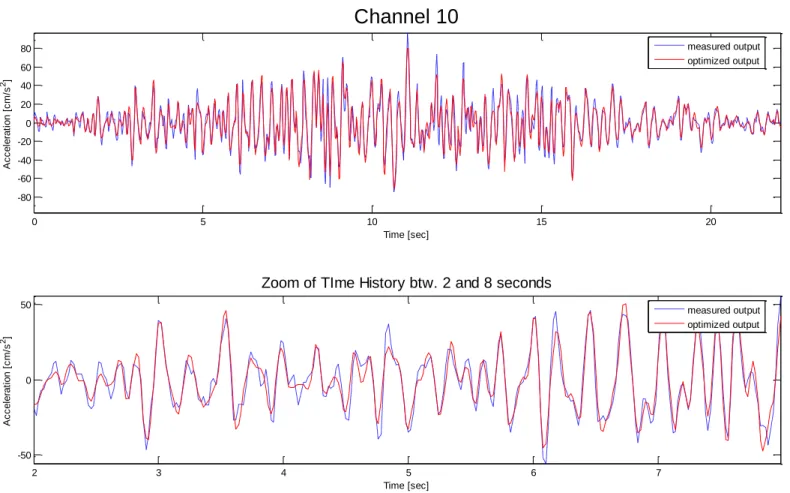
Da tali modelli possono essere facilmente ricavati i parametri modali della struttura, quali le frequenze, i rapporti di smorzamento e le forme modali. Tale approccio d‟identificazione si basa sull‟utilizzo dell‟Eigensystem Realization Algortihm (ERA), complementato dall‟algoritmo Observer/Kalman filter IDentification (OKID). Per l‟ottenimento dei risultati finali, si attua un‟ottimizzazione tramite la minimizzazione dell‟errore tra la risposta dedotta computazionalmente e quella misurata. L‟analisi dei risultati porta a concludere che la metodologia qui proposta è efficace nell‟identificare le caratteristiche strutturali del sistema, sebbene si debba riconoscere che tali risultati potrebbero essere migliorati avendo ad esempio a disposizione time histories più lunghe o accelerogrammi registrati anche sulla sponda sud del ponte.
Fin dall‟inizio della sua introduzione, molti utenti hanno trovato questo metodo efficace in numerose applicazioni pratiche nel contesto del controllo delle vibrazioni di strutture flessibili in campo aerospaziale e meccanico. La teoria, dunque, è stata originariamente coniata appositamente per questo tipo di sistemi, tuttavia la formulazione matematica si basa su ipotesi facilmente applicabili a qualsiasi tipo di struttura.
35
3.1 Introduction
In the field of identification of structures, the common practice is to create an analytical model and to update it by using static and dynamic testing. The initial finite element model is calibrated by comparing the numerical eigendata (natural frequencies and mode shapes) with the eigendata acquired from the model tests. Approaches based on frequency response functions and fast Fourier transforms are still dominant in the model updating philosophy. The aim of experimental modal analysis is to retrieve the system‟s modal characteristics, such as the natural frequencies, mode shapes, etc. from experimental data. However, such experiments generally require a large number of actuators and sensors to pick up most of the modal data. An alternative approach to determine an appropriate structural model is to use input-output relations, as the one developed in the present work.
The time histories available at the Center of Engineering Strong Motion Data (CESMD) are necessary to the Observer/Kalman filter Identification (OKID) algorithm to compute the Markov parameters of the system. The quality of the estimated state of the system by a designed observer depends on the accuracy of not only the assumed system model, but also the assumed system and measurement noise characteristics. Information of both the system and the noise characteristics are embedded in the above mentioned Markov parameters. For a lightly damped system, the number of system Markov parameters needed to be solved for becomes exceedingly large. It is known that not all the system Markov parameters are independent. By invoking the Cayley-Hamilton theorem we know that every Markov parameter can be expressed as a linear combination of a finite number of “independent” system Markov parameters where the unknown coefficients of the linear combination are those of the system characteristic equation. The key issue is how to reduce the number of unknowns without having to pose this problem as a non-linear parameter estimation problem. It is possible
36
to compress the original set of system Markov parameters into another set of parameters where the details of the compression is explained via a special matrix, which is precisely an observer gain described previously.
The observer Markov parameters are then used by the Eigensystem Realization Algorithm (ERA) to realize the discrete time first order system matrices. Then, via a non-linear optimization algorithm, the output error between the measured and detected response is minimized. Finally, the physical characteristics of the structure are recovered by means of a technique discussed by Lus (2001) and De Angelis (2002).
For my purposes I have used one of the latest version of the function OKID/ERA/non-linear optimization algorithms written in the Matlab programming language. Essentially, the user provides a set (or multiple sets) of input-output data, together with such information as the number of inputs, the number of outputs, sampling interval, etc., the function will return an identified state-space model, associated observer gain and physical characteristics of the model.
37
3.1.1 The Historical Path of OKID/ERA Algorithm
During the last three decades, there has been a vast number of studies and algorithms concerning the construction of state space representations in the time-domain for linear dynamical systems, beginning with the works of Gilbert and Kalman. One of the first result obtained in this field was about „minimal realizations‟, indicating „a model with the smallest state-space dimension among system realized that has the same input-output relations within a specified degree of accuracy…‟. It was shown by Ho and Kalman, that the minimum representation problem was equivalent to the problem of identifying the sequence of real matrices, known as the Markov parameters, which represent the unit pulse responses of a linear dynamical system. Following a time-domain formulation and incorporating results from control theory, Juang and Pappa proposed an Eigensystem Realization Algorithm (ERA) for modal parameter identification and model reduction of linear dynamical systems, which extends the Ho-Kalman algorithm and creates a minimal realization that mimics the output history of the system when it is subjected to unit pulse inputs. Later, this algorithm was refined to better handle the effects of noise and structural non-linearities, and the ERA with data correlations (ERA/DC) was proposed. When general input data such as an earthquake-induced ground motion is used, difficulties in retrieving the system Markov parameters can arise related to problem dimensionality and numerical conditioning. Among the algorithms proposed to overcome these difficulties, the Observer/Kalman filter IDentification (OKID) algorithm introduces an asymptotically stable observer which increases the stability of the system and reduces the computation time, improving the performance even when the noise and slight non-linearities are present. This technique has proven to be quite successful in the aerospace community in the identification of complex, high-dimensional space craft structures.
38
3.2 Basic Formulation
3.2.1 Input-Output relations
The dynamic behavior of an N degrees of freedom linear structural system can be represented by the second-order differential equation:
) t ( ) t ( ) t ( ) t ( Lq Kq u q M B (3.1)
where q ϵ RN is the structural displacement vector in a fixed system of reference. The matrices M, L and K, all RN x N, are the mass, damping and stiffness matrices, respectively, while B ϵ RN x r indicates the continuous time input matrix, in fact, the vector u(t) is assumed to contain r external excitations applied to the system. When the input is represented by a seismic excitation, the components of q(t) correspond to nodal displacements with respect to a system of reference whose origin is at the base of the structure and moves together with the base. The external forcing term B u(t) can now be replaced by MINx1xg(t), with IN x 1 being the unitary vector and xg(t) the ground acceleration at the time t.
The same structural system of equation (3.1) can also be represented as a system of first-order differential equation in state-space form, setting v(t)q(t):
) t ( ) t ( ) t ( ) t ( ) t ( ) t ( q v u q K v L v M B (3.2)
Let assume that one is provided of only m output time histories of the response, then, it is possible to introduce a new vector y(t), containing the measurements available (generally m ≠ N).
39
T T a T v T p (t) (t) (t) ) t ( 0 ) t ( ) t ( 1 0 ) t ( ) t ( q Ψ q Ψ q Ψ y M B v q M L M K v q (3.3) ) t ( ) t ( ) t ( ) t ( ) t ( ) t ( u D x C y u B x A x (3.4) (3.5)where x is the n-dimensional state vector, and y is the m-dimensional output vector, where n is 2N. The matrices A ϵ Rn x n, B ϵ Rn x r, C ϵ Rm x n and D ϵ Rm x r represent the time invariant system matrices. Since we receive measurements of input and output as sets of discrete data, it is convenient to work in the discrete time domain so that equation (3.4) and (3.5) can be expressed as difference equations in the following form:
) k ( ) k ( ) k ( (k) (k) 1) (k u D x C y u Γ x Φ x (3.6) (3.7)
where the integer k denotes the time step number, i.e. x(k+1) =x[k(T)+T], with
T being the time step interval. Assuming the input as a unit pulse, we obtain:
Γ Φ C C Γ Φ Φ Γ Φ Φ 1 n-n n 1 n-1 n n 1 2 1 x y x x 1 n k for x x 1 k for 1 x 0 k for (3.8)
The yn are called system Markov parameters, they are the response of the system
40
discrete time system matrices and can be evaluated as = eA(T) , so that
= B
DT A d e 0 , and the solution of equations (3.6) and (3.7) is given by the
following convolution sum:
1 1 0 1 1 0 x( ) x(0) y( ) C x(0) D
k k k j j k k k j j k u(j) k C u(j) u(k) (3.9) (3.10)For zero initial conditions, equation (3.10) can also be written in matrix form for a sequence of l consecutive time steps as:
l l r l r m l m M U Y (3.11) where
y(0),y(1),y(2), ,y(l 1)
l m Y (3.12)
D CΓCΦΦ CΦ Γ
Mmrl , , ,, l2 (3.13) ) 0 ( u ) 1 ( u ) 0 ( u ) 2 l ( u ) 1 ( u ) 0 ( u ) 1 l ( u ) 2 ( u ) 1 ( u ) 0 ( u l l r U (3.14)the matrix Y is a matrix whose columns are the output vectors for the l time steps, while the matrix U contains the input vectors for different time steps arranged in an upper-triangular form. The matrix M contains the Markov parameters, in form of its partitions. The system Markov parameters form a basis for the ERA.
41
3.2.2 Observer/Kalman filter IDentification
The aim of this paragraph is that of explaining how to extract the system Markov parameters when only input-output data are available. The first attempt would be that of solving equation 3.11. However, for a input multiple-output system the solution of that system is not unique, unless one truncates the Markov parameters sequence. In addition, deciding at which order truncate that sequence is problematic as well, especially for lightly damped structures. OKID algorithm solves these issues by introducing an observer to the state space equations, so that equations 3.6 and 3.7 become:
) k ( ) k ( ) k ( (k) ˆ (k) ˆ ) k ( ) k ( ) ( ) k ( ) ( u D x C y Γ x Φ Ry u RD Γ x RC Φ y(k) R -y(k) R u(k) Γ x(k) Φ 1) x(k (3.15) (3.16) where:
T T
T (k) (k) (k) ˆ ˆ y u ν R RD Γ Γ RC Φ Φ (3.17)The new matrix R is chosen in order to make the system of equations 3.15 and 3.16 as stable as possible. The gained system can be considered as an observer system, therefore its Markov parameters are called observer Markov parameters. By choosing R such that Φˆ is asymptotically stable, one can obtain the result
0 ˆ ˆhΓ
Φ
C for h > p, and the input/output relation can be written as:
(r m)p r (r m)p r l m
l
m Mˆ V
42
The observer Markov parameters are the block partitions of the matrix Mˆ , and
they are obtained by finding the least-squares solution of Equation 3.18 as:
Mˆ =Y V† (3.19)
with ()† denoting the pseudo-inverse of a matrix. It should be noted that when both Y and V are polluted with noise, the least square solutions might be problematic. Moreover, since the Markov parameters of the real system are retrieved from the identified observer Markov parameters, any bias introduced in the initial least-squares solution might propagate and become more pronounced in the Markov parameters of the real system, leading possibly to loss of accuracy in the final identified model. Having identified the observer Markov parameters, the system Markov parameters can be retrieved using the recursive formula:
D ˆ ˆ ˆ (2) k l i k 1 k 0 i ) 2 ( i ) 1 ( k k M M M M M
(3.20)Once the system Markov parameters have been identified, they can be used in the ERA formulation for the identification of the dynamic structural characteristics.
43
3.2.3 Eigensystem Realization Algorithm
The objective now is solving the so called minimal realization problem, i.e. finding a set of minimum order discrete time matrices , C, D, from the system Markov parameters identified previously.
Let us consider that r impulse tests have been performed on a system with
m outputs. Let us denote with yj(k) a new vector, of dimension m, that represents the response of the system at time kT to the unit impulse input uj at time zero. In
this way, we can package the data as:
y y y
Y(k) 1 2 r (3.21)
For definition given in the first paragraph of this chapter, the vector Y(k) represents the system Markov parameters at time k t. The evaluation of the matrix D is then very simple, since it is apparent that:
) 0 (
Y
D (3.22)
Having identified the D matrix, we now look for C, . ERA solves the problem by means of the singular value decomposition of the Hankel matrix, an
ms x rs matrix constructed by means of the system Markov parameters just
identified: )] 1 s ( 2 k [ Y symm ) s k ( Y ) 2 k ( Y ) 1 s k ( Y ) 1 k ( Y ) k ( Y ) 1 k ( s H (3.23)
44
where s is an integer that determines the size of such a matrix. The Hankel matrix is a block symmetric matrix: denoting with O~ the ms x n the observability matrix and with C~ the n x rs controllability matrix, the Hankel matrix can be written as:
C O~ ~ ) i ( Φi H (3.24) where:
T T T C 1 s 2 T 1 s T 2 T ~ ) C ( ) C ( ) C ( ~ C O (3.25) (3.26) Γ CΦ Γ CΦ Γ CΦ Γ CΦ Γ CΦ Γ CΦ H ) 1 s ( 2 i s i 2 i 1 s i 1 i i symm ) i ( (3.27)The rank of the Hankel matrix is equal to the dimension of the minimum realization. The singular value decomposition of the Hankel matrix can then be written as:
T 1 1 T 2 T 1 2 1 ~ ~ ) 0 ( U S V V V 0 0 0 S U U UΣΣ H T C O (3.28)where the matrices U, of ms x ms dimension, and V, of rs x rs dimension, are unitary matrices, while the diagonal matrix S encloses exactly n singular values for a system deprived of noise. It is then clear the statement of the ERA theorem:
45 † † H Φ V S S U C O C O ~ ) 1 ( ~ ~ ~ T 1 2 / 1 2 / 1 1 (3.29)
where ()† denotes the pseudo-inverse of a matrix. The input matrix can be easily determined, as it is the first block partition of C~, and, similarly, the output matrix
C is the first block partition of O~.
3.2.4 Refining the Identified State-Space Model
The method described in the preceding sections performs quite well for finite-dimensional system when:
1) the available input/output data time histories are sufficiently long; 2) the noise is white, of zero mean and small.
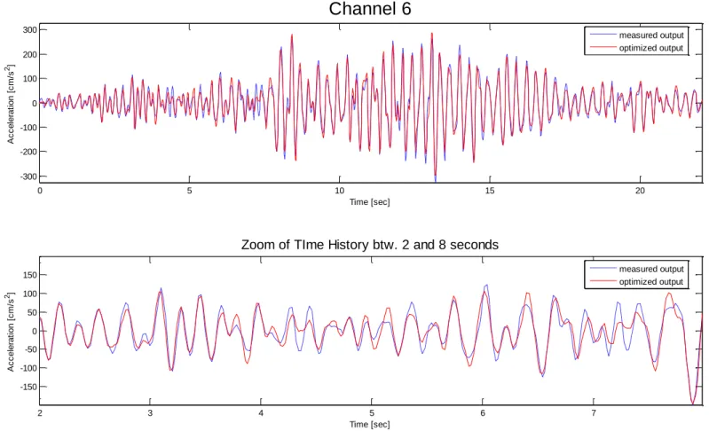
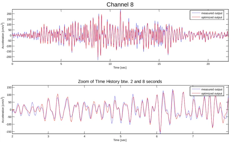
When these conditions are not satisfied, the results could be not acceptable. Moreover, measurement noise is not the only issue one has to consider. Other problems such as non-stationary and insufficient excitations, and truncation errors introduced in the ERA stage, also contribute to the errors. Therefore, it is apparent that the basic OKID/ERA methodology needs an optimization. The technique used to obtain the results of the present work is the output error minimization approach, a non-linear least squares problem based on the minimization of the following function:
L k i T )] k ( ) , k ( [ )] k ( ) , k ( [ 2 1 ) ( y y y y F (3.30)where contains the parameters to be optimized, the vector y(k,) is the output vector obtained from the state-space realization at time-step k, while y(k) is the
46
measured output at time step k, with the index k varying from an initial time ti to a
final time tf.
In particular, the method used for the optimization of the state-space realization is the „Sequential Quadratic Programming‟ (SQP) technique, belonging to the quasi-Newton-type methods family; such methods guarantee fast convergence provided that the initial conditions are sufficiently close to the desirable solutions. This issue is solved for the problem analyzed, since the solutions provided by the methodologies discussed previously will serve as reasonably good estimates to initiate the search.
The Taylor series expansion truncated at the second order of equation 3.30 is:
) ( ) ( ) ( ) ( T 2 1 H G F F (3.31)
where, for i referring the ith output, the following terms have been considered :
) ( ) , k ( ) , k ( ) ( ) ( ) , k ( )] k ( ) , k ( [ ) ( ) ( T tf ti k 2 L k i T
y y y y y F H F G (3.32)
tf ti k m 1 i i 2 i i ) , k ( y )] k ( y ) , k ( y [ ) ( (3.33)It is necessary to have the Hessian at worst positive semi-definite, therefore, the contribution of only the positive eigenvalues of () to H() will be considered. The SQP technique is an iterative method: in each iteration the parameters are updated via the following formula:
) ( )] ( [ dj * j 1 T j j 1 j H G (3.34)
47
where j denotes the jth iteration, dj is the step size, and H*(j) and GT(j) are
obtained by evaluating Equations (3.32) using the parameters j. The size of the
iteration step size has to be calibrated in order to avoid any instability, and to have a decrease of the objective function F().
An important issue is the choice of the parameters to be optimized. It can be observed that the observer Markov parameters play a crucial role in the identification of the state-space realization, and then, indirectly, to the determination of the dynamics of the system, that are the proper objectives of the whole identification. Of course, one could decide to optimize all of the variables in the discrete time state space matrices, and in that case the number of elements of would be n2 + n x r +m x n. This approach would give reliable results, but the
computational effort requested will be very high for complex structures. An alternative is represented by the transformation of the state space discrete time system realization to a set of modal coordinates. Since the eigenvalues of the identified first-order system appear in complex conjugate pairs as ~i ji, with j representing the imaginary unit, the discrete time equations can be transformed into a new basis in which they can be written as n/2 uncoupled equations (one for each structural vibration mode) as
(k) (k) (k) (k) (k) ) 1 (k B B B Du z C y u z z where: (3.35) 2 / n 2 / n 2 / n 2 / n 2 2 2 2 1 1 1 1 B ~ ~ 0 0 0 0 ~ ~ 0 0 0 0 0 0 ~ ~ 0 0 0 0 ~ ~ 0 0 0 0 0 0 ~ ~ 0 0 0 0 ~ ~ (3.36a)
48 mr 1 m r 1 11 2 / n , r 1 2 / n , 21 2 / n , r 1 2 / n , 11 1 , r 2 1 , 21 1 , r 1 1 , 11 B d d d d , D (3.36b) 2 / n , 2 m 2 / n , 1 m 1 , 2 m 1 , 1 m 2 / n , 12 2 / n , 11 1 , 12 1 , 11 B c c c c c c c c C (3.36c)
and the state vector can now be expressed as z(k)[zT,1(k)z,nT/2(k)]T. With this formulation, the total number of parameters is reduced to n + n x r + m x n + m x
r. The discrete time equations for each mode in the state vector can now be
written separately as:
) t ( D ) t ( ) t ( ) t ( ) t ( ) t ( 1 u z C y u B z Λ z (3.37)
where in are embedded the continuous time eigenvalues of the identified state space model, while , of order n x n, is the matrix of the eigenvectors corresponding to the eigenvalues of .
49
3.2.5 Recovering the dynamics of the system from the realized
state-space model
Finally, it is possible to retrieve the dynamics of the system using the optimized state-space realization 3.37. Let recall the well-known eigenvalue problem:
2iMiLK
i 0 (3.38) where i represents the ith complex eigenvalue i = i± jI, for i = 1,2,…, N. Theeigenvectors are then scaled such that:
I Λ ψ ψ 0 M M L Λ ψ ψ (3.39)
Λ ψ ψ M -0 0 K Λ ψ ψ (3.40)where is the matrix containing the complex eigenvalues, while the one of the corresponding eigenvectors. By using the assumptions presented in equations 3.39 and 3.40, the system of equations 3.4 and 3.5 becomes:
(t) (t) (t) (t) (t) p T ξ ψ y u ψ Λξ ξ C B (3.41)
that represents the first order modal form of the equation of motion 3.1. Formulation given by equations 3.41 is a different model of the same system represented by equations 3.37: there must be a transformation matrix T that relates the two representations:
50 ψ ψ Λ Λ p 1 1 C T C B B T T T 1 -T 1 - (3.42)
Once the eigenvectors matrix is determined, the evaluation of the mass, damping and stiffness matrices are retrievable from equations 3.39 and 3.40:
1 1 ) ( ) ( T T T ψ Λ ψ K M ψ Λ ψ M L ψ Λ ψ M 1 -2 (3.43)
and undamped natural frequencies and damping ratios can be finally calculated:
i i i i i 2 i 2 i i arctan cos 2 f (3.44)
51
3.3 Numerical Results
The Painter Street Overcrossing was instrumented in 1977 by the California Division of Mines and Geology as part of the California Strong Motion Instrumentation Program. The bridge site was instrumented with twenty strong accelerometers capturing various motions on and off the bridge as shown in figure 3.1. Channels 12, 13 and 14 measure free field motions (longitudinal, vertical and transverse to the bridge axis respectively) near the bridge site. At the east end of the bridge, triaxial sets of sensors are located both on the embankment (15, 16, 17) and on the end of the bridge deck (9, 10, 11) so that relative motion between the embankment and the deck could be assessed. A triaxial set of sensors (1, 2, 3) is also located at the base of the bent‟s north column to aid in measuring soil-structure interaction. A transverse sensor (7) is located at the base of the deck adjacent to the center bent and vertical sensors are located at midspan of the east (8) and west (6) spans on the north side of the deck. An important issue is the absence of accelerometers at the south edge of the bridge: torsion of the bridge cannot be directly assessed.
Since the overpass was instrumented, it has been shaken by six earthquake. Of these only three set of data are available at Center of Engineering of Strong Motion Data (CESMD). Therefore, the results herein proposed are obtained by using records of Trinidad Offshore, Rio Dell earthquake and the first event of Petrolia earthquake. Table 3.1 presents the characteristics of the six earthquakes that interested the structure since 1977.
In figure 3.1 are circled in different colors the sensors whose records are used as input and output data. In particular, the sensors circled in red offer input data, while the ones circled in blue give the output data.
52
Event Date Mag.
[ML] Epic. Dist. [km] Maximum Ground Acceleration Maximum Bridge Acceleration C12 C13 C14 C6 C7 C8 Trinidad 11/08/80 6.9 72 0.15g 0.03g 0.06g 0.34g - 0.25g Rio Dell 12/16/82 4.4 15 - - - 0.39g 0.43g 0.59g Cape Medoncino 08/24/83 5.5 61 - - - 0.27g 0.22g 0.16g Petrolia (#1) 11/21/86 5.1 32 0.46g 0.08g 0.16g 0.24g 0.26g 0.33g Petrolia (#2) 11/21/86 5.1 26 0.15g 0.02g 0.12g 0.21g 0.36g 0.29g Cape Medoncino 07/31/87 5.5 28 0.15g 0.04g 0.09g - 0.34g 0.27g
53
54
3.3.1 Trinidad Offshore (November 8, 1980)
For this set of data records from channels 1, 2, 3, 15, 16, 17, 18, 19, 20 are used as inputs, while the ones from channels 5, 6, 8, 9, 10, 11 as outputs. The total number of data points for each record is 1104, at a sampling interval of 0.02 seconds.
As discussed, the choice of the number of observer Markov parameters affects the solution of the observer system, and then it is critical in the determination of the characteristics of the structure. It is important to choose the value of the number of observer Markov parameters (denoted as ‘p’ from now on) as higher as possible. The upper bound for p is given by the following demonstrable formula:
73 r m r l pmax (3.45) where r = number of inputs (9) m = number of outputs (6) l = number of data points (1104)
The number of system Markov parameters is usually set from two to four times the one of p. In the present work ‘nmarkov’ (number of system Markov parameters) equals four times p.
With the values of ‘p’ and’ nmarkov’ defined, it is now possible to run the OKID/ERA via MATLAB. The program needs the asks for the definition of other parameters. The first thing one has to choose is the number of singular values of the V*VT matrixto keep to compute observer Markov Parameters. Usually, it is chosen the number of singular values just above the sharp drop, that in this case equals 1031. Nonetheless, after many trials, it has been observed that for this set of data the most stable results are
55
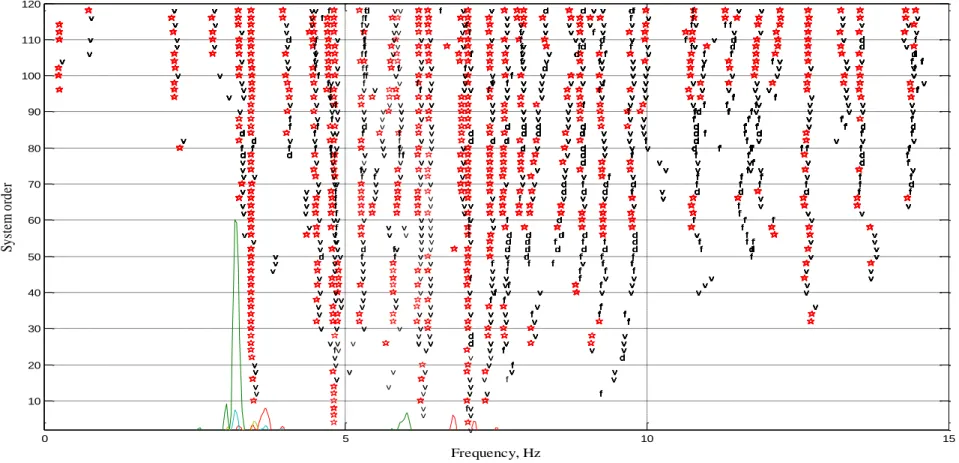
obtained by keeping 558 singular values, whose amount is one of the first to be not negligible (Figure B.1). The next step is to choose the number of singular values of the decomposed Hankel Matrix H(0)*H(0)T (Figure B.2). When output observations are not contaminated by noise, the dimension of the state matrix can be clearly indicated by singular values of H(0)*H(0)T and so the modal parameters for the system modes can be estimated just from a realized model. However, when output measurements are disturbed by noise, the Hankel matrix has full rank and this makes it difficult to assign a certain order to an identified system model only based on the singular values distribution. Even though it is true that having a higher order identified model helps in minimizing the error between the measured data and the reconstructed responses from the identified model, this error reduction could be due to noise modes that are now included to improve the fitting between the data sets. For this reason the extraction of modal parameters corresponding to structural modes is generally complemented by a Stabilization Diagram (SD). Such a diagram, which represents the identified frequencies as a function of the model order, highlights modes whose properties do not change significantly when varying the dimension of the state vector; such modes are considered as structural modes. In order to form the SD, an observability matrix is repeatedly formulated from equation 3.29 varying the dimension of the state, which provides different pairs of state and output matrices of corresponding orders. The properties of poles in a model of a certain order are compared with those of a two order larger model and stable and unstable modes are determined on the basis of the identified frequencies, damping ratios and mode shapes. A star in the diagram represents a value for which modal shape, frequency and damping are stable; an ‘f’ indicates that only modal frequency is stable, while a ‘v’ should give stable modal shape and frequency; finally, a ‘d’ informs that modal frequency and damping are stable (Figure 3.1).