38
Chapter 4
VALIDATION OF VEHICLE MODEL AND
ANALYSIS OF THE RESULT
4.1. The vehicle model simulator
4.1.1. Introduction to CarMaker®
CarMaker® is a commercial software that allows to simulate and analyze the global dynamical behavior of four-wheel vehicles; it also enables a wide spectrum of applications besides the classical vehicle dynamic simulation: describing the dynamic of a vehicle in response to a particular input set (steering angle, longitudinal speed, etc.), testing and developing a chassis control system, reproducing tough driving maneuvers also thanks to a fully parameterized driver model, analyzing the vehicle’s consumption and other applications normally used for virtual test driving. This software is mainly composed of five integrated modules described below [21], [22].
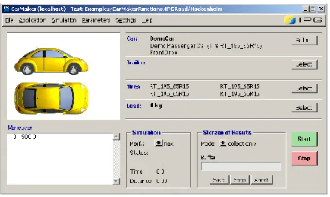
Figure 4-1 – CarMaker GUI
The main module “CarMaker GUI (Graphical User Interface)” (Figure 4-1) primarily serves as user interface: it represents the control center of CarMaker;
39
through this module different characteristic parameters of the vehicle and simulations (road, maneuvers, driver model, etc.) are settable.
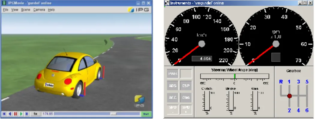
The IPGMovie (Figure 4-2, left) is the CarMaker’s animation tool for online (during a simulation) or offline use (reading of result files).
The third module “Instruments” allows displaying graphically the most useful data of a vehicle, especially the tachometer. The content is very similar to what is present in the cockpit of a real car (Figure 4-2, right).
Figure 4-2 – CarMaker IPGMovie and Instruments
The “IPGControl” module allows plotting and viewing the result of a simulation. From Figure 4-3, it is possible to see that there are a huge number of simulation variables which can be plotted. It allows also manipulating these, changing the scaling, axis, etc. so that the results can be better analyzed.
40
The fifth module is a program system called “IPGKinematics” designed to simulate a vehicle axle on an axle kinematic test bench and is used to calculate the kinematics, steering kinematics and elastokinematics of all types of suspension. Additionally to all the previous modules, the CarMaker software features an interface for both of the most important result management tools, Excel and Matlab.
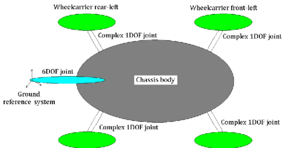
Figure 4-4 – Joints and rigid bodies within the vehicle model
The multibody system used in the software consists of five rigid bodies interconnected by five rigid joints (Figure 4-4). The rigid bodies may move in space and relative to each body. The chassis body is connected to the ground body with a six degree of freedom joint (cyan-blue color). The wheel carrier bodies are connected with the chassis body with a complex one degree of freedom joint (white color), which simulates the suspension. The model described has therefore ten degrees of freedom.
4.1.2. Setting the vehicle’s parameters
To run a simulation it is necessary to build a model. This can be done having access to the GUI and then to Parameters > Car in order to open the vehicle editor. After having created and saved a default vehicle data set, the Vehicle Generator has to be used. This is a tool that generates automatically a plausible vehicle data set,
41
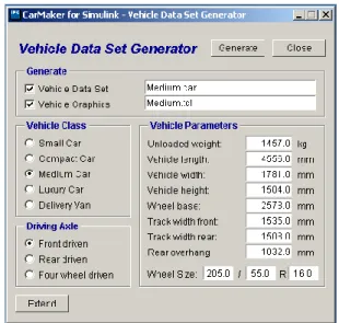
based on the most important data that characterizes a vehicle. It’s possible to select directly the class of the vehicle, e.g. “Compact Car” or “Luxury Car” in order to get the typical values corresponding to this kind. Here, the basic characteristic of the Volkswagen test car presented in Table 3-1 will be introduced. The results are shown in Figure 4-5, where also length, width, height, track width front and track width rear of the vehicle appear:
Figure 4-5 – Vehicle Data Set Generator
After this, a new vehicle is generated, and it is possible to work with the new vehicle data set: from now on, the new values previously inserted are not only displayed in the editor, but also really saved. Then, it is necessary to parameterize the vehicle, e.g. tyres, suspensions, etc.. The following subsections refer to the various sections of the vehicle editor.
4.1.2.1. Main Body
First of all, the vehicle model wanted is chosen by using the option “kind”: RigidBody – a simple vehicle model without flexibility;
FlexBody – a model with a feasible body.
A RigidBody is chosen to simplify the model: in fact, nothing can be said about the flexibility of the body. With this choice, the vehicle will be constituted only by one
42
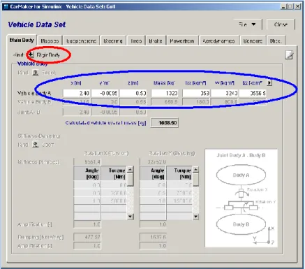
body, which is called “Vehicle Body A”, as shown in the Figure 4-6 (red circle). In the blue circle there are the main characteristic of the Vehicle Body A: they are the
position of the center of gravity respect the reference system (located as shown
in Figure 4-7), unloaded mass of the vehicle, and the three vehicle moment of
inertia respect the position of the three axis of the reference system.
Figure 4-6 – Vehicle Data Set: selection of a rigid body
43
It is worth remembering how these quantities were obtained: the position of the center of gravity is known from Table 3-1; the vehicle mass was measured with four scales which were situated underneath each tyre [23]; for the two moment of inertia the default values of a CarMaker medium car were chosen, instead the
moment was previously estimated as reported in [24].
4.1.2.2. Masses
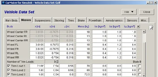
As shown in Figure 4-8, in this tab all the other masses of the vehicle are defined, according to the model chosen in the “Main Body” tab. They are:
Engine: this value is optional, since the engine mass can be merged with the body masses; no value was therefore entered;
wheels: unsprung spinning masses;
wheel carriers: unsprung masses that don’t rotate;
trim loads: additional loads which can be added to the Vehicle Body. The three masses of passengers who were sitting in the car during the tests in the proving ground belong to this category (so three trim loads are defined);
44
4.1.2.3. Suspensions
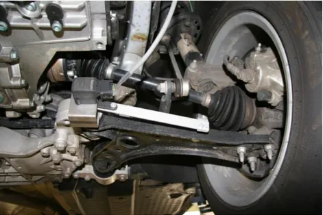
The Volkswagen test car is characterized by a MacPherson strut in the front axle and a four link suspension in the rear axle. They are respectively shown in Figure 4-9 and Figure 4-10. Springs, dampers, buffers, stabilizers and kinematics of both suspensions are modeled in the next sections.
Figure 4-9 – Volkswagen front axle: MacPherson strut
45 4.1.2.3.1. Springs
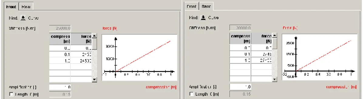
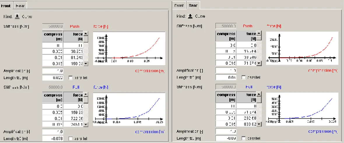
In this tab the spring stiffness for the front and rear axle are independently defined. The stiffness has to be indicated in N/m. In this case, a linear characteristic for the spring is chosen, in accordance with Table 3-1. This is a simplification: the presence of other additional elastic elements will be taken into account with the parameterization of buffers. The choice both for front and rear spring is shown in Figure 4-11.
Figure 4-11 – Springs parameterization, front and rear
4.1.2.3.2. Dampers
In this tab the damping factor for the front and rear axle are independently defined. The damping has to be indicated in Ns/m. Push and pull domain are separately parameterized: in particular, the damping factor is here greater in extension than in compression to allow a fast dissipation of energy stored within the spring during the extension and to get a not very high force during the compression. However, also here a linear characteristic for the dampers is chosen, in accordance with Table 3-1. The Figure 4-12 shows the characteristics of the two dampers, and for both push and pull are separately shown.
46
Figure 4-12 – Dampers parameterization, front and rear
4.1.2.3.3. Buffers
The buffer enables to limit the wheel travel. If the wheel travel reaches the given distance, the buffer acts like an additional spring. Because of the lack of data about this element, it has been decided to use the default values contained in the commercial software. These values are shown in Figure 4-13, where front and rear, push and pull, are separately considered.
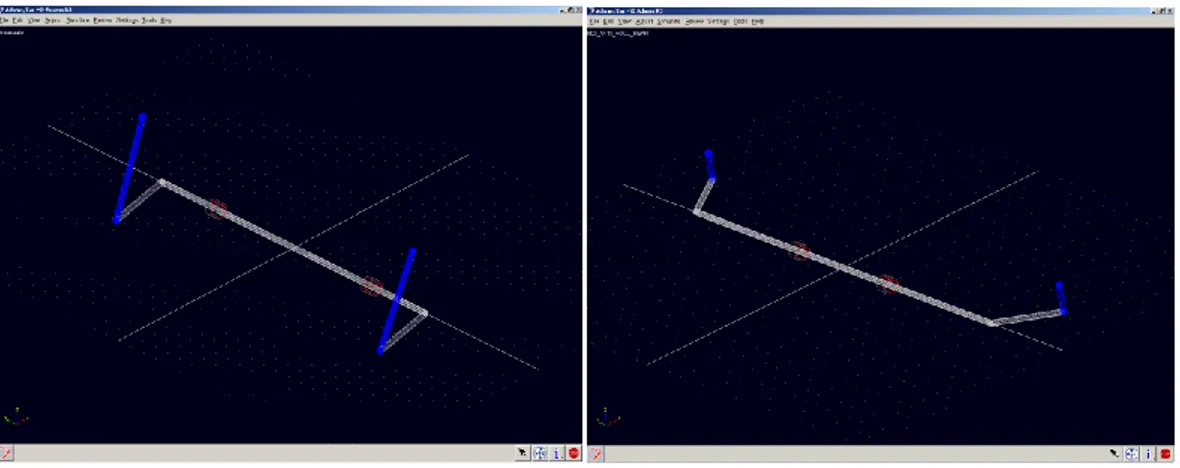
47 4.1.2.3.4. Stabilizers
Figure 4-14 – Stabilizer bars model in AdamsCar, front and rear
Two AdamsCar models of front and rear stabilizer bars were previously created as reported in [25]. They are shown in Figure 4-14.
First of all is necessary to calculate the stabilizer bars stiffness, which has to be entered in N/m. The calculation is reported in Appendix A. The front and rear
stabilizer stiffness and respectively are:
They are entered in CarMaker as shown in Figure 4-15:
48 4.1.2.3.5. Kinematics
CarMaker offers a kinematics model where it is not necessary to parameterize the geometry of the vehicle axle; in fact, the only important information are the positions of the wheels according to the wheel travel and the steering rack displacement (for the front axle only). As a more accurate alternative it is possible to parameterize the entire axle kinematic by tables written to an external file. This possibility is given by the IPGKinematics program which was briefly introduced in 4.1.1.. In order to have a more accurate parameterization of the front axle, this alternative is chosen; indeed, for reason of modeling simplicity, a “linear” kinematic characteristic is chosen for the rear axle: in this case, the kinematic only depend on the wheel travel and it is parameterized by coefficients directly introduced in the vehicle editor.
Considering the front axle, the following quantities were set:
1. Parallel Compression simulation type: is the possibility to have a simulation where left and right wheel suspensions are jounced and rebound in the same direction. This option will be used;
2. Distance of extension-compression, from a minimum to a maximum value (±65 mm with a stepsize of 5 mm);
3. Reciprocal Kinematics simulation type: in this case the left and right wheel suspensions are alternately jounced and rebound. This option will not be used;
4. Steering Kinematics simulation type: in this case the steering rack is displaced (CarMaker considers a rack-and-pinion steering system): the front wheels are then correspondingly steered. This option will be used to simulate the steering system kinematics;
5. Lateral Force simulation type: it applies a specified force in the vehicle’s transverse direction at the left and right force application point of each wheel. This option is used for both wheel (left and right): in this case it is also necessary to specify the minimum and maximum values of lateral force (±7000 N with stepsize of 250 N);
6. Longitudinal Force simulation type: same characteristics than the previous simulation type but a longitudinal force is applied in the tire force application point. This option will not be used;
49 7. Vehicle data which are subdivided into:
General: this section mixes parameters of the overall vehicle with specific design features: Driving Torque Ratio (100% because the front axle is driven); Tire Rate (the vertical stiffness of the tire [N/mm] is calculated in Appendix B); Wheel Toe and Camber angle (not considered).
Springing: entered in this tab are the parameters for the axle spring and stabilizer bar: Spring fixing and Stabilizer bar fixing (which element carries respectively the spring and the stabilizer bar: in this case both are fixed to the wheel carrier), Type of axle spring (linear in this case), Spring Rate (24,5 N/mm), Torsional Rate of the stabilizer bar (292 Nm/deg). Some of this input values are repeated (they were entered during the construction of the main model) because IPGKinematics operates as a separate sub-program which does not take into account the car parameterization.
Bushings: an input file is specified for each bushing, with the file containing all of the information on a bushing. It is possible to switch between the individual bushings of the wheel suspension; the content of the tab are then updated accordingly and the parameters for the selected bushing are displayed. Due to lack of information about bushing structure, position, shape, force, damper rate and torsional spring rate, it was not possible to make a modeling of those, so that the IPGKinematics default bushings were selected.
Masses: all unsprung masses are introduced. Due to lack of information , the IPGKinematics default values were introduced; Geometry: here, the positions of all elements which forms the
50
Figure 4-16 – Reference system for the definition
of MacPherson geometry
A local reference system for the front axle is used: its origin and
the direction of its axis is shown in Figure 4-16. To insert the coordinates of the elements in this reference system, a AdamsCar® front suspension model was used. This was previously created as reported in [25]. Figure 4-17 clearly represents the MacPherson model: the numbers in yellow dots refer to the elements mounting positions and are reported in Appendix C.
Figure 4-17 – MacPherson model in AdamsCar [25]
The position of all the elements in the Adams model was therefore
transformed in the local reference system and the new coordinates
were entered in IPGKinematics. The geometry obtained can be graphically controlled by the “Graphical Control” button. The positions of all points of the wheel suspensions are represented to
51
scale. The Figure 4-18 contains three views: Sectional view, Side view, Top view of the MacPherson front suspension:
Figure 4-18 – CarMaker Geometrical Control
Integrated with “IPGKinematics” is “IPGGraph” which allows displaying the suspension kinematics results. Between the huge amount of graphics which can be plotted with this tool, it is interesting to show the trend of camber angle and toe angle with the left wheel
travel (the translation of the wheel center in Z direction) in case of a
parallel compression. They are shown in the following Figure 4-19 and Figure 4-20.
Figure 4-19 – MacPherson front suspension, variation of camber angle
52
Figure 4-20 – MacPherson front suspension, variation of toe angle with left wheel travel
From the Camber angle plot, it is possible to see that such angle has higher alteration (positive values) when the wheel is in rebound conditions (>2 deg); furthermore, the wheel is in condition of toe-in during the spring compression.
For the rear axle the IPGKinematics program was not used: the reason is that the Multi-Link rear suspension is characterized by a too high level of complexity which cannot be correctly managed by the program. Different simulation were tried but with poor results. A so called “Linear2D” kinematics was used: in this particular case the suspension kinematics depend on the wheel travel and the movement of the opposite wheel and the parameterization is obtained by entering coefficients in
the tables of vehicle editor. Here, the and parameters respectively
define the translations and rotations of the wheel in three directions (i.e. represents the camber angle variation and is the toe angle variation). Because of the lack of information about such quantities, a CarMaker default rear kinematics was chosen ( = 0.02 rad, = 0 rad).
53
4.1.2.4. Steering system
In CarMaker the relation between the steering wheel angle or the steering wheel torque and the steering rack displacement has to be defined (the so called “steering ratio ”). This relation can be linear or non-linear: a linear relation is here chosen and the steering ratio, previously calculated, is = 14.96.
4.1.2.5. Tyres
As already described in 3.3.1.4., a Magic Formula tyre model is used. An Adams tire property file is supported by CarMaker: it contains a list of parameters, introduced in the previous chapter, which defines the tire property. They are obtained using the Cftool of Matlab and entered in the Adams property file: the tyre model is then created.
Four different tyre models were considered at the beginning, which are: WRG2 1.8 bar, WRG2 2.2 bar, RF 2.2 bar and RF 3.0 bar. Four different Adams property files were therefore written. They are shown in the Appendix D.
4.1.2.6. Powertrain
The test car has a TDI engine of 1.9 liters, which can provide a maximum torque of 250 Nm at 1900 rpm and a maximum power of 77 kW at 4000 rpm.
In CarMaker, the powertrain is a global system which is divided into a number of subsystems with defined interfaces. These are: Kind, Engine, Clutch, Gearbox and Driveline.
4.1.2.6.1. Kind
The “Powertrain – Kind” selects the kind of torque generation, which can be: Generic for a common internal combustion engine, OpenXWD used for a hybrid driveline and AVL_Cruise which is a very detailed powertrain modeled by AVL. A Generic kind is chosen.
4.1.2.6.2. Engine
The engine model is primarily concerned with engine torque. It provides the torque to the clutch input shaft. An engine torque “map” which represents the torque
54
characteristic can be prepared and entered in CarMaker. The real 1.9 TDI engine torque map is available in the technical internet page of Volkswagen [26]. This is therefore entered in CarMaker: the result is shown in Figure 4-21:
Figure 4-21 – 1.9 TDI engine torque map and CarMaker parameterization
4.1.2.6.3. Clutch, Gearbox and Driveline
CarMaker offers the possibility to parameterize a manual clutch as well as an automatic transmission. Same possibility for the gearbox, where two models are available: manual and automatic. Default CarMaker clutch and gearbox were selected, as missing sufficient data to build these two subsystems.
Regarding the option “Driveline”, it enables to choose the kind of transmission: front, rear or any kind of 4WD. A front transmission is here considered.
4.1.3. Definition of the maneuver
Several maneuvers can be run in the software; basically every kind of simulation may be simply obtained. However, as first step is necessary to validate the model: this is possible considering the real data acquired in the Nokia test track; in particular, CarMaker offers the possibility to use such real measurements as input to define a maneuver. Several data may be read from a file: vehicle longitudinal speed and steering wheel angle are the most important: they will be entered as input in the software.
55
The next Figure 4-22 shows the “Input from a file” dialog box where real measurements data are entered:
Figure 4-22 – Input from a file dialog box
In “Input File” the measurement file is loaded. It contains three columns to represents three different channels: time, longitudinal speed, steering wheel angle. This file can be created importing the measured data files in a text file. The “Time Channel” box defines the time channel which will be the main one followed by the program during the simulation. In “Starting Conditions” the starting speed, gear and gas position are used as initial values. The “Model Quantity to override” is a list of quantities which may be overwritten: the values for the selected quantities are read directly from the file and used as given by CarMaker.
4.1.4. Definition of the scenario
In this paragraph, the parameters required to define the road model are described. The road model of CarMaker is called “IPGRoad” and is reachable from the GUI. This model enables to build an open or closed track in CarMaker.
56
The window showed in Figure 4-23 represents the first section of IPGRoad, which is General Settings: through it, is possible to enter the global settings which will be applied to the whole track.
Figure 4-23 – IPGRoad tab
They are:
Start coordinates: it defines the origin of the middle of the road;
Car starts at (m): it defines at which distance the car should start (normally is set to 0);
Track Width: it defines the width of the entire track on both sides of the middle lane; here the friction coefficient is also defined, e.g. 1.0 for a good macadam or 0.1 for a icy surface; a value of 1 is considered here;
Margin Width: it defines the lateral zones of the road where usually the friction coefficient is lower; therefore a different coefficient has to be introduced here: a value of 0.6 is considered;
With regard to the definition of the road geometry, it consists of a succession of various segments (straight lines, curves, etc.) with parameterized properties in order to build a complete road. This method is defined in the section “Segments” as shown in Figure 4-24:
57
Figure 4-24 – Definition of the road geometry in IPGRoad
The segment list is displayed in the green circle: here they are added or deleted. In the red circle it is possible to define the exact tridimensional geometry of each segment, setting the following quantities:
Kind of Segment: it defines the general geometry of the segment selected (a curve, a straight line, etc.);
Length: it defines the length of the segment and it is used only for straight lines;
Angle (deg) and Radius (m): they are two parameters used to describe curves;
Grad (%), Slope (%), Camber (m/m): they enable to define each segment in
three dimensions: Grad defines the longitudinal slope, Slope define the
lateral slope, Camber defines in [meters of elevation/meters of lateral
58
4.2. Simulation results and comparison
4.2.1. Validation maneuver
As already discussed in 3.2.2., the first maneuver tested is a double-lane change at a start speed of 108 km/h: it is representative of the transient lateral behavior of the vehicle. So in the input file will be loaded a text file obtained from Nokia proving ground measured data: in that case, the double-lane change maneuver was tested with RF 2.2 bar tyres on the front axle and WRG2 2.2 bar tyres on the rear axle, so this justified the name given to the input file in Figure 4-22. Nevertheless, a measure unit conversion is necessary: the longitudinal velocity extracted from the measurement is expressed in km/h, so that the signal has to be multiplied for a quantity that is 0.277 to obtain the same quantity in m/s; the steering wheel angle has a negative value, so it has to be multiplied for -1. The starting speed is 107.2 km/h and the gear engaged is the fourth.
As road definition, a “black lake” was created: it consists in a scenario where a straight segment of 2000 m defines a track whose width is > 50 m on left and right sides, the car starts at a distance of 200 m from the beginning, the friction coefficient between tyres and asphalt is set to 1. In these conditions, the car moves on a wide asphalt surface without reaching the external margins. The following Figure 4-25 better clarify such concept:
59
Figure 4-26 and Figure 4-27 respectively show the yaw rate and vehicle slip angle trend during the test, and compares experimental data with CarMaker results:
Figure 4-26 – Yaw rate trend during double-lane change maneuver
Figure 4-27 – Vehicle slip angle trend during double-lane change maneuver
Figure 4-26 and Figure 4-27 are representative of the good match there is between simulation and experimental data: it is possible to understand the goodness of the model built with CarMaker.
60
Other quantities can be compared (e.g. Lateral acceleration, Lateral speed, etc.) but the figures are not here shown.
4.2.2. Steering-pad
Steering-pad tests were performed in Nokia proving ground for six different combination of tyres and pressure, as already discussed in the previous 3.2.3.3. Every combination was tested two times to obtain clockwise and counterclockwise maneuver: it is worth remembering that directly from this maneuver is possible to extract the handling diagram.
Six input data files were created and run; the starting speed was 0 km/h and the gear engaged was the first: only first and second gears were used during the test, so that in CarMaker gearbox subsystem only two gears are selected.
About the simulation scenario, the circle of 40 m of radius was reproduced in CarMaker. To obtain this, a “Turn right” segment was used for angle of 360 deg; the radius was set to 40 m, a small lateral slope was considered (0.2%), to simulate the real track geometry. Friction coefficient was set to 1, and the track width was set to 6 meters both sides. Figure 4-28 shows the CarMaker steering-pad simulation running in the case of WRG2 tyres on front axle and WRG2 tyres on rear axle.
61
The pictures from Figure 4-29 to Figure 4-31 show different Yaw rate trends for the six different set of tyres, and a comparison between experimental data and CarMaker results. A Counterclockwise maneuver is only considered.
Figure 4-29 – Yaw rate comparison: A) WRG2 2.2 bar front – WRG2 2.2 bar rear; B) RF 2.2 bar front – WRG2 2.2 bar rear
Figure 4-30 – Yaw rate comparison: A) WRG2 2.2 bar front – RF 2.2 bar rear; B) RF 2.2 bar front – WRG2 1.8 bar rear
Figure 4-31 – Yaw rate comparison: A) RF 3.0 bar front – WRG2 1.8 bar rear; B) RF 2.2 bar front – RF 2.2 bar rear
62
4.2.2.1. Handling diagrams
By using the signals of steering angle, longitudinal speed and yaw rate extracted from Carmaker simulations, six handling diagrams are created. The equation (2.14) was used. The diagrams obtained by simulations are directly compared with the six experimental handling diagrams showed in 3.3.2.1. Pictures from Figure 4-32 to Figure 4-34 show such comparison:
Figure 4-32 – Handling diagrams comparison: A) WRG2 2.2 bar front – WRG2 2.2 bar rear; B) RF 2.2 bar front – WRG2 2.2 bar rear
Figure 4-33 – Handling diagrams comparison: A) WRG2 2.2 bar front – RF 2.2 bar rear; B) RF 2.2 bar front – WRG2 1.8 bar rear
63
Figure 4-34 – Handling diagrams comparison: A) RF 3.0 bar front – WRG2 1.8 bar rear; B) RF 2.2 bar front – RF 2.2 bar rear
Some difference can be noticed at high lateral acceleration (>±0.8 g): the CarMaker model doesn’t reach such high level of lateral acceleration and when this is reached the difference between steering angle and Ackermann angle becomes noisy, as it is shown in Figure 4-32 A and B and Figure 4-33 B.
However, the comparison immediately shows the close proximity between the experimental data obtained on the track and the simulations.
4.2.3. The driver model
After having validated the CarMaker model by using real measurements, a driver model is defined. The aim is to create new simulations and therefore new handling diagrams without using inputs from a file, but customizing the behavior of a virtual driver: in fact, the previous data were obtained from real measurements and were particularly noisy; the driver model uses also certain inputs, has feedback from the car and environment to know if the vehicle is doing what he intended to do, generates outputs to the vehicle as steering angle, longitudinal speed etc. These quantities are more precise and smooth.
64
4.2.3.1. Driver parameters
In order to repeat the steering-pad maneuvers using a virtual driver model, the driver parameters were entered in the tab; the most important of them are shown in Figure 4-35.
Figure 4-35 – Set the driving parameters
Mode: in order to drive on any tracks with different driver characteristics, a “User parameterized driver” is chosen. The “Racing Driver” mode, after a learning phase, calculates the physical limits of the driver considering very high speed and accelerations: very important becomes the aerodynamics behavior of the vehicle. Limit conditions were tested at the Nokia proving ground, but the User parameterized driver was used.
Cruising speed: it is the speed that the driver will try to reach, keeping the vehicle on the track. It is set to 80 km/h (the maximum speed reached during the steering-pad maneuvers is 75 km/h);
Max. Long. Acceleration and Deceleration, Max. Lat. Acceleration: they define the driver’s maximal value of acceleration (lateral and longitudinal) and longitudinal deceleration. To repeat the same conditions of acceleration during the test at the proving ground, a longitudinal acceleration of 0.258
65
m/ and a maximal lateral acceleration of 10 m/ are chosen; for the
construction of the handling diagrams, no importance is given to the
deceleration (a default value of -6 m/ is considered). These limits define a
“G-G diagram” which is shown in the following Figure 4-36:
Figure 4-36 – G-G diagram
Declutching/Gear Shifting: it defines the time necessary to shift up or down the gears. It is set to a ideal value of 0.001 sec.
4.2.4. New set of tyres
The previous tyre models described in 4.1.2.5. are used to create the new handling diagrams. Together with these, new tyre models were introduced. They are: WRG2 2.6 bar, WRG2 3.0 bar, RF 1.8 bar, RF 2.6 bar. The tyre parameterization for these models is described in the Appendix D.
66
Combination Set Front axle Rear axle Tire Pressure (bar) Tire Pressure (bar) A A1 WRG2 1.8 WRG2 1.8 A2 WRG2 2.2 WRG2 1.8 A3 WRG2 2.6 WRG2 1.8 A4 WRG2 3.0 WRG2 1.8 B B1 WRG2 1.8 WRG2 1.8 B2 WRG2 1.8 WRG2 2.2 B3 WRG2 1.8 WRG2 2.6 B4 WRG2 1.8 WRG2 3.0 C C1 WRG2 1.8 RF 1.8 C2 WRG2 2.2 RF 1.8 C3 WRG2 2.6 RF 1.8 C4 WRG2 3.0 RF 1.8 D D1 WRG2 1.8 RF 1.8 D2 WRG2 1.8 RF 2.2 D3 WRG2 1.8 RF 2.6 D4 WRG2 1.8 RF 3.0 E E1 RF 1.8 WRG2 1.8 E2 RF 2.2 WRG2 1.8 E3 RF 2.6 WRG2 1.8 E4 RF 3.0 WRG2 1.8 F D1 RF 1.8 WRG2 1.8 D2 RF 1.8 WRG2 2.2 D3 RF 1.8 WRG2 2.6 D4 RF 1.8 WRG2 3.0 G G1 RF 1.8 RF 1.8 G2 RF 2.2 RF 1.8 G3 RF 2.6 RF 1.8 G4 RF 3.0 RF 1.8 H D1 RF 1.8 RF 1.8 D2 RF 1.8 RF 2.2 D3 RF 1.8 RF 2.6 D4 RF 1.8 RF 3.0
67
4.2.5. New handling diagrams
According to the previous Table 4-1, new handling diagrams are created. It is important to remember that such new graphics are completely obtained by the simulation software, which uses a car model and a driver model.
The handling diagrams are reported in the picture from Figure 4-37 to Figure 4-40.
Figure 4-37 – CarMaker handling diagram: 1) Combination A; 2) Combination B
68
Figure 4-39 – CarMaker handling diagram: 1) Combination E; 2) Combination F
Figure 4-40 – CarMaker handling diagram: 1) Combination G; 2) Combination H
4.2.5.1. Discussion
From the previous pictures is possible to notice the frequent understeering behavior of the vehicle; for a normal front driven car an increase of the understeering behavior with the lateral acceleration is wanted. But there are some exceptions in the previous diagrams. This is discussed as follows:
the choice of set of tyres for the rear axle is very important; in fact, mounting a WRG2 set in the rear axle gives always an understeering behaviour of the vehicle, for every kind of front set of tyres and every
69
pressure (this is the case of combinations A, B, E, F in Figure 4-37 and Figure 4-39);
mounting a RF set of tyres to the rear axle can give different results (combinations C, D, G and H in Figure 4-38 and Figure 4-40); here the most important parameter is the tyre inflation pressure: increasing it to the front axle tyres gives always a understeering behaviour (C and G. The vehicle is more understeering with the increase of pressure); instead, increasing it to the rear axle can give an oversteering behaviour (D and H. The vehicle is less understeering with the increase of pressure; it becomes oversteering at 3.0 bar);
it is important to remember also that the two oversteering conditions (both for RF at the rear axle) are obtained at a tyre pressure of 3.0 bar: this value is uncommon for the normal drive conditions (the tyre pressure is kept around a value of 2.2÷2.3 bar) during which the vehicle is always in understeering conditions;
there is almost no difference between handling diagrams obtained at a pressure of 2.2 bar and 2.6 bar. Around these to limit values the behaviour of the vehicle stays the same.