146
CHAPTER 4
IMPLEMENTATION OF A CORE
INVOLVING 3 PMA32’s
4.1 MULTIPLEXING ON A
RING INVOLVING 3 PMA’s
This paragraph is a meditation on the possible topologies that can be created using 3 PMA-32’s.
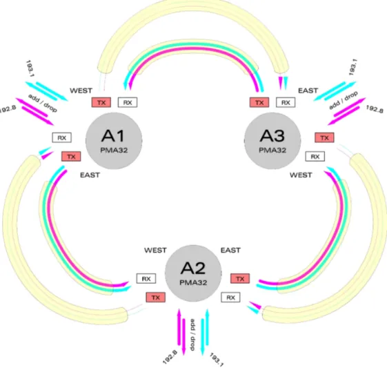
First of all let’s just have a look at an ideal scenario: 3 PMA’s, which have been all configured with the Worker on the west line, so to have a real ring topology – in every PMA32 the main traffic can be received (dropped) at the East RX and sent from the West TX, or we can also decide to have a simple pass-through not having any add/drop action. This solution can be seen in Figure 4.1.
147
In the picture we have considered a possible add/drop procedure at the 3 PMA’s, using 2 tributaries – the pink and the blue ones, which are shown as the 192.8 and the 193.1, that is to say the 2 frequencies we have considered in the tests faced throughout the Chapter 3 experience.
Obviously we can decide where to add and where to drop a certain frequency, thus selecting also where we want a certain PMA to let a frequency be passed through: for example we could add the blue wavelength at the A1 PMA, select a pass-through at the A3 PMA, and finally drop it at the A2 PMA, or at the sourcing A1 itself – as we prefer or as we need.
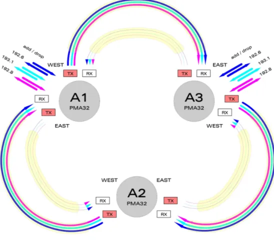
So we see the way all the system works: in this scenario the direction is the WEST one, but we can SWAP WORKER/PROTECTION to obtain the opposite goal – using the EAST direction. Actually we can see in Figure 4.2 the way this can be done, obviously when no SIGNAL FAIL ON PROTECTION alarms are raised for the frequencies we’re working on.
Figure 4.2 – Ring involving 3 PMA’s with Worker at the East TX for every single PMA
This was a general resume of the possible scenario an operator could create or manage; it’s important to highlight that, even if the PMA features are quite useful and repetitive as for the procedures required to change a topology or to face a signal failure problem, a ring with 3 PMA’s is not as practical as a point-to-point link with 2 PMA’s, which is much more manageable and elastic to necessities or topology changes – actually this is the way the Marconi technology is thinking its new apparatuses, thus following more linear and simple strategies.
148
Anyway we must remember how the ring topology can be useful in metropolitan area networks: here’s the reason why we’re considering in the next paragraph a real 3 PMA’s scenario on which many tests have been faced.
4.2 THE PHYSICAL LAYER GOAL:
A 3 PMA’s OPTICAL CORE
4.2.1 CONFIGURATION OF THE 3 INVOLVED PMA’s
In this section we’re finally examining an optical core implemented with the 3 PMA’s we have been testing throughout the Chapter 3 of this publication.
Our goal was to create a topology including a dedicated fiber link connecting two locations in the city of PISA, 2 PMA’s situated in the locations themselves, plus a PMA used to add more complexity to the link and to implement the pass-through feature.
The real scenario we have finally created is just like the ideal one shown in Figure 4.1. The only thing we have to say is we’re adding 3 frequencies at the A1 PMA, dropping them and adding them again at the A3 and finally dropping them at the sourcing A1 PMA itself – all using the Spirent AX 4000, so to compare the results with the ones we got in the 2 PMA’s case. Everything is shown better in Figure 4.3.
149
Actually it should be an interesting thing to see the impact a new PMA (in our case the A2) can have on the link – and we’re going to understand it later in this section.
The A1 is, as usual, the PMA situated at the Information Engineering Department, and the A3 & A2 are located in the CNIT block, in S. Cataldo’s area, in the same room connected to each other as if they were connected at a certain distance.
Besides we could also add or drop the one or two frequencies at the new A2 PMA, but it could be done only moving one of the two cards available for a certain frequency or for both frequencies – but this would be unnecessary in a topology as the one we have created, where the A2 and A3 PMA’s are in the same location, connected to each other by very short fiber cables, which add a very small delay.
What we have done to use the third PMA without any cards involving the two usual 192.8 and 193.1 tributaries is creating a pass-through for the two frequencies – as we know the pass-through just forwards a certain traffic received at the EAST RX onto the WEST TX, and any traffic received at the WEST RX onto the EAST TX – thus not doing any action on the treated flows.
At the A1 and A3 PMA’s we have configured cross-connections for 3 frequencies: the 192.8 and 193.1 Gbit Ethernet traffics and a 192.6 frequency available for the ATM/SONET traffic. In the tests we’re going to face we’re focusing on the 2 Gbit Ethernet flows, during the transmission of the 3 frequencies obtained multiplexing them in a unique signal.
Let’s start with a quick description of the standard windows available for the A1 PMA, showing the hardware and the eventual alarms regarding the cards inserted in the PMA itself (Figure 4.4, 4.5)
150
As we can see in the pictures there’s no red alarm regarding the east or west TX / RX, while there can be something indicated in red if some of the used frequencies cannot be sent in the correct way throughout the ring. The Controller/Comms device (Figure 4.4) and the shelf monitor (Figure 4.5) are alarmed in red because there are some warnings or not important alarms noticed in the hardware by the considered cards ( as we’re going to see in the alarms pictures shown later in this paragraph).
As for the SQM device, it’s alarmed in red for a problem due to a lightly different value of a monitored wavelength if compared with the one expected by the system (nothing problematic).
Figure 4.5 – Sub-rack configuration @ A1 PMA
In Figure 4.5 we can see in which slots the 3 tributary cards have been located.
It will be also useful for an operator to use the View Cable feature to see the internal cabling and the frequencies which have been associated to the cards located in the chosen slots (Figure 4.6).
There are some slots we’re not going to use, that we have to associate to a certain frequency just because they are adjacent to the slots hosting our cards and frequencies – for those empty slots we can select some random frequencies chosen among the ones not involved by the system at the moment.
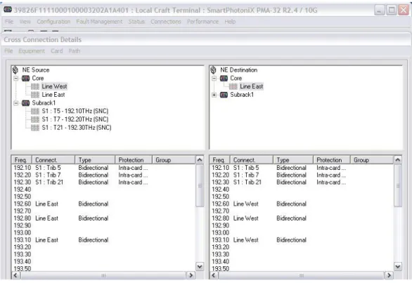
Always considering the first PMA we can have a look at the Connections window, resuming all the frequencies and the cross-connections / pass-through’s created on the present PMA (Figure 4.7).
In this case we see 3 pass through connections created for the 192.1,192.2, 192.3 frequencies, due to three protected cards contained in the A2 PMA, not used at the moment.
151
Figure 4.6 – Sub-rack cabling @ A1 PMA
Figure 4.7 – Cross-connections window @ A1 PMA
The Amend SNC Protection window, analyzed in Chapter 3 in the section regarding the protection features, is very useful to decide where to send what frequency at each PMA, getting eventual alarms regarding the tributaries’ incapability to follow the required path. We’re now having a look at the following A3 PMA, situated at the other end of the long link.
152
Figure 4.8 shows the Signal Quality Monitor graphics, where we can view all the wavelengths which are being treated by the system – this could be really immediate and useful when sending a large number of flows.
The SQM is useful but not necessary in a PMA32, so one could decide to locate a SQM only on a PMA, and not to the others. Actually we’ll not find a device like that in the sub-racks of the A3 & A2 PMA’s.
Figure 4.8 – Signal Quality Monitor – available @ A1 PMA
153
Figure 4.9 refers to the A3 PMA’s sub-rack, and the red alarm signaling the T13 tributary regards the Loss Of Signal problem at the west TX affecting the west 192.8 channel, as already seen when testing the point-to-point link between A1 & A3 in Chapter 3.
We’ll see later that this problem will not let our topology work as we projected it, so we’ll be forced to send the 192.8 frequency onto the east direction at the A3 TX side.
Figure 4.10 – Remote mode, Cross-connections window @ A3 PMA
154
In Figure 4.10 we show the connections available at the A3 PMA, so to go on with the clear comprehension of the projected links among the apparatuses.
192.1, 192.2 and 192.3 are the 3 frequencies related to the 3 cards located in the A2 PMA; besides we have the 3 usual cross-connections.
Figure 4.11 starts the description about the last PMA, the A2 – which has 3 protected cards, as already explained above.
We’ll notice in the next picture (Figure 4.12) that in this PMA the 192.1, 192.2 and 192.3 tributaries have been configured as cross-connections, while the remaining 3 frequencies - the ones cross-connected in the preceding PMA’s – are now considered simple pass-through’s because they’re not added or dropped at this node of the network.
Figure 4.12 – Remote mode, Cross-connections window @ A2 PMA
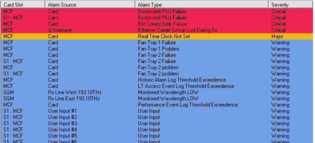
With the preceding picture we have finished the resume about the 3 PMA’s configuration. A final help to the reader is given showing the alarms noticeable at the 3 apparatuses. In the next page we can compare the 3 Real Time Alarms windows obtained in the 3 PMA’s (Figures 4.13, 4.14, 4.15) and notice that EM Comms Link Failure & Distributed PSU Failure are common red alarms – and we have already explained how these two problems are signaled by the PMA but they do not create any particular problem in the system.
Power Feed Failure A is an alarm signaling that one redundancy module bringing electricity to the A3 PMA has failed – so it should be replaced; but we haven’t done that considering that some PMA’s do have this redundancy system while others don’t use it. Wrong card fitted is finally an alarm signaling that the PMA notices a slot with a card/configuration mismatch, but it depends on a faulty slot, which appears to have a card inside while it’s empty at the moment. Otherwise it’s common in the PMA-32 to see from time to time some cards which are inserted but not recognized by the management software or some signaled cards which are not really located in the corresponding slots: it’s one of the negative characteristics of this apparatus (we have noticed this on all the considered PMA’s).
155
Figure 4.13 – A1 real time alarms
Figure 4.14 – A3 real time alarms
Figure 4.15 – A2 real time alarms
4.2.2 LATENCY VALUES IN THE POSSIBLE TOPOLOGIES
In the present paragraph we’re going to test once again the delay values which are obtained using the different paths between the transmitters and receivers of the A1 and A3 PMA. The values will be compared with the ones we got in the point-to-point link, to see what changes in this case – thus verifying the additional delay given by the new A2 PMA.
Let’s start with the standard configuration shown in Figure 4.16, which has the west TX selected at each PMA for each frequency: the selected path was a medium delay in the point-to-point link considered in Chapter 3.
156
The desired configuration is not available because of the problem involving the A3 WEST TX, so the system will force the 192.8 frequency to the east direction at each PMA – as the DUAL ENDED MODE has been selected. We can easily verify this in Figure 4.17.
Figure 4.16 – The desired configuration, with all the frequencies on the external path
Figure 4.17 – The configuration as it can be configured by the PMA’s
To calculate the packet transfer delays we’re using the Spirent AX4000, which generates traffic and analyzes it at the A1 PMA situated at the Information Engineering Dept.
157
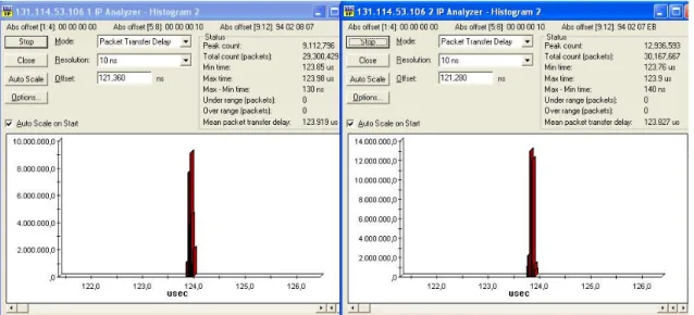
Let’s see the results we get in the scenario shown in Figure 4.17, with the 192.8 frequency running on the eastern path (left histogram) and the 193.1 frequency passing through the west direction (right histogram) (Figure 4.18).
Figure 4.18 – Medium path delay for both Gigabit Ethernet traffics
The delay seems to be more or less the same using the east or the west path: 123.9 and 123.8 – actually it was like that even in the 2 PMA’s scenario, as we can see in the following Figure 4.19 (2 paths with approximately the same delay transferring the packets).
Figure 4.19 – Comparison delays obtained in the 2 PMA’s configuration
Comparing the 2 Figures 4.18 and 4.19 we’ll notice that the new A2 PMA adds a delay which is around 1 microsecond, so a really small delay if we consider that a medium fiber link as the one considered (about 20 Km) creates a 123 microseconds delay – this means we could add many PMA’s to a fiber ring absolutely not caring about the delays this could add to the configuration.
Obviously we expect the frequencies to have the same kind of delay values when sending all tributaries on the east direction – the 192.8 will not change its path, while the 192.6 and 193.1 will go on the opposite direction than before (Figure 4.20).
158
Figure 4.20 – Medium path delay for both Gigabit traffics using the opposite direction
An interesting test is sending the 192.6 and 193.1 on the west direction at both PMA’s once again, forcing the 192.8 frequency to be sent on the west direction at the A1 PMA and to be sent back on the east direction at the A3 PMA, so not letting the 192.8 Worker pass through the A2 PMA – this should generate for the 192.8 tributary the usual shortest path delay we saw in the last chapter (Figure 4.21).
159
Comparing Figure 4.22 and 4.23 we get about the same 104.5 microseconds delay in each case a frequency is sent through the west TX at the A1 PMA and using the east TX at the A3 PMA.
As we have already said many times this is the shortest path to send a traffic onto the ring we have created, and it can be easily used in every case we are not interested in adding or dropping any frequency at the A2 additional PMA.
Figure 4.22 – Shortest path for the 192.8, medium path for the 193.1
Figure 4.23 – Comparison delays obtained for the 2PMAs configuration’s shortest path
Finally we can also send all the frequencies between the west part of the A1 and the east part of the A3, thus excluding the the channels called “Workers”.
In a situation like that the path starting at the east part of the A1 and getting back at the west part of the A3 will be a protection channel for all the frequencies, which will be passed through the A2, where as we know a pass-through has been initially configured. In this case we’ll find a 104 microseconds delay for both the 192.8 and the 193.1 Gigabit Ethernet tributaries (Figure 4.24), the exact value we got using only two PMA’s (actually nothing has changed in this configuration if compared to the one used in the last chapter).
160
Figure 4.24 – Shortest path for both the 192.8 and the 193.1 tributaries
To complete our analysis we must measure the delay for the path which connects the east TX at the A1 with the west TX at the A3 – obviously considering the usual problem on the 192.8 when sending traffic on the west direction.
If we consider the single ended mode for the 192.8 tributary we’ll have the topology shown in Figure 4.25 and the results of Figure 4.26.
161
We’ll measure a 142 microseconds delay, exactly one microsecond more than in the point-to-point link topology, for the 193.1 tributary, and about 123 microseconds for the 192.8 frequency, which uses the internal path.
Figure 4.26 – Longest path for the 193.1; single ended & medium delay for the 192.8
Considering the dual ended mode we’ll have the 192.8 tributary running on the shortest path, so getting a delay of about 104 microseconds, the usual good path – not passing through the A2 PMA (Figure 4.27 and 4.28).
162
Figure 4.28 – Longest path for the 193.1; dual ended & shortest delay for the 192.8
Let’s just focus on a final scenario, with 3 more frequencies, the 192.10, 192.20, 192.30 – related to 3 cards we have in the A2 PMA and we haven’t used until now.
This way we could have 6 frequencies multiplexed in a unique signal by the PMA32’s. Whatever number of frequencies we use, the delays will be more or less the same as the ones considered in the tests above; so it should be useful to resume all the results in the following Figure 4.29, where the “VS” indication stands for a comparison with the delays we got in Chapter 3 in a point-to-point link.
163
4.3 COMPUTER NETWORKS BASED
ON OPTICAL CORES with PMA’s
4.3.1 AN ADD-DROP OPERATION REQUIRING 2 FREQUENCIES
Sometimes it could be useful to consider two different frequencies for a single add-drop operation involving a certain kind of traffic (in the next paragraph we’ll use a video traffic): for example if we wanted to have a particular traffic passing through the optical ring, and getting back to the place where the source itself is, we could use a tributary card, working at a certain frequency, to send the signal onto the ring and another card using another frequency to receive, or better drop, the signal getting back from the ring.
We could for example send the signal onto the ring using the 192.8 frequency, get through the link between our Engineering Department and the CNIT, and finally drop the traffic using the 193.1 frequency – so we’ll be able to decide which direction to choose depending on the delays we need to have and on the topologies we want to create.
To better learn the way this operation can be implemented by our PMA’s, we can have a look at Figure 4.30.
164
In this scenario we are using two frequencies, the 192.8 and 193.1 tributaries; the add operation is done at the A1 PMA, and we have chosen the point-to-point link structure, so that the A2 PMA (where there’s a simple pass-through for both frequencies) seems to be unused at the moment – actually it’s being passed-through by the protection lines.
The main file transfer involves the upper part of the picture.
We have chosen to add the pink frequency at the A1 PMA, simulating to drop it at the A3 PMA - actually we have connected the 192.8 “drop” fiber to the 193.1 “add” fiber, so at the A3 PMA it’s just as we were dropping a certain traffic, and adding another one by another frequency. So two traffic flows are being transferred on opposite directions, even if in this case the two file transfers involve the same signal and not two separate traffics.
Obviously at the A1 PMA we’ll also drop the blue frequency to verify the latency values and the quality of the signal – this can be done using an application as VLC, which seems to be easy to use and clear about the main parameters we need to transfer a simple video traffic from a computer to another one.
We cannot talk about a real multiplexed signal in the case we’re examining, because in the picture above we can see how starting both at the west tx line @ A1 PMA, and at the east TX line @A3 PMA we’ll have a single transfer channel fully used for the traffic sent (indicated by a continuous line), plus the feedback channel (indicated by a broken line) of the opposite frequency – and we must not forget that the feedback channel, even if necessary to let the transmission be successful, is not a fully used optical channel.
We’ll see in the next sections a scenario where a real multiplexed system implements the DWDM philosophy.
4.3.2 CONFIGURATION OF THE NETWORK/TRANSPORT LEVELS
In the last paragraph we’ve seen the problems and the goals related to the PMA itself, that is to say we’ve analyzed the level 1 of the ISO protocol stack.
It’s surely interesting to highlight that following the complexity of a computer network, as we’re going to do in these sections, the PMA is to be seen as nothing more than a cable connecting a certain network in a certain seat to another network at another place – in our case we have a network which is going to be configured at our Information Engineering Dept. and a second one at the CNIT structure.
So the level 1 of the protocol stack is about the computers we’re going to use and the PMA’s on the ring, also considering the fiber cables that implement the logical topology. Level 2 involves the level 2 switches connecting the different computers on a specific network; while level 3 includes the IP addresses used for the test.
Level 4 is the one we’re caring about now, and involves the routers – actually we’re using a single Juniper router, configured as two logical routers.
The two logical routers are the only way to let an operator send and receive the traffic in the same location (in our case at the A1 PMA).
Figure 4.31 explains better the network configuration we have chosen to communicate between the Information Engineering Department and the CNIT.
An address has been chosen for each of the two PC’s, for each connection between two instruments, and for each router interface.
As we can see in the picture, we are using two fast Ethernet copper interfaces to connect the two PC’s to the router (shown ideally as two different routers) and two Gigabit Ethernet optical interfaces to connect the router (ideally the two logical routers) to the ring
165
made of 3 PMA’s. This way all the interfaces have their own address and some pings can be done to verify that the router configuration has been properly created.
Levels 3 and 4 have now been correctly configured – next we’re going to see an interesting application which will let us test and verify the file transfer.
166
4.3.3 DOUBLE FILE TRANSFER ON OPPOSITE DIRECTIONS
In the last sections we saw how to send a single traffic flow throughout the ring testing the quality of the received signal – everything using 2 frequencies for the same traffic.
What we’re going to do now is imagining to add a flow and drop the opposite flow at each PMA.
There are two main topologies available for our ring: the point-to-point link (Figure 4.32) and the complete ring (Figure 4.33).
Between the two the better one is the point-to-point link, because, as we verified in chapter 3, it offers a shorter delay than the ring topology.
What we have tried to make clear in the two pictures shown is that even if the topology changes we always have a transfer channel (continuous line) and a feedback channel (broken line) for each frequency’s Worker. Besides we’ll have the same thing in the protection lines (thin lines).
The feedback channel is necessary to have the connections established, otherwise the system would not work.
Figure 4.32 – Double File Transfer on opposite directions with Point-to-Point Link configuration
167
Figure 4.33 – Double File Transfer on opposite directions with Ring configuration
4.3.4 MULTIPLEXED TRAFFIC FOR A DOUBLE FILE TRANSFER
To complete the different kinds of topology we could create using the 3 PMA’s we have configured, let’s have a look at Figure 4.34.
This time we have two add operations at the A3 PMA and two drop operations at the A1 PMA – so finally we’re using a real multiplexed signal on the ring.
The multiplexed transfer involves the 192.8 and the 193.1 frequencies, which are being sent at the east TX at both PMA’s (we have thus chosen the complete ring topology) – and we have a multiplexed main channel and a feedback channel as usual.
We’re sending in this case two parallel traffics - as for example two videos, starting at the CNIT structure – and receiving them at the Information Engineering Department.
In our tests, to have clear explanations and proper schemes, we’ve used only two Gigabit Ethernet traffic flows, but the PMA can multiplex, as we know, many different flows - up to 32 – so that we could simulate up to 32 file transfers with the chosen topology.
168
Figure 4.34 – Multiplexed signal created with two traffic flows on the same direction
Besides many different LAN’s could be connected by routers to the optical core: here is the big goal the PMA can reach. Let’s also remember that the delay a single PMA can add to a complex system as the one we’re using is about 1 microsecond: practically nothing considering that the bottlenecks would be others at this point – such as the fast Ethernet interfaces or the applications used on a PC.
169
4.4 PMA-32 AS OPTICAL CORE
FOR A GRID COMPUTING TESTBED
The optical core we have implemented by the 3 PMA-32’s mentioned throughout the book has been included in a testbed for Global Grid Computing – with the idea of better explaining the Topology Discovery methods – these methods are going to be analyzed in this paragraph.
4.4.1 GLOBAL GRID COMPUTING
Global Grid Computing is mainly used to connect heterogeneous computational resources belonging to the same Virtual Organization (VO) through the Internet to form a unique and more powerful virtual computer.
To fulfill this goal it is necessary to develop services that provide the virtual computer with the same functionalities of individual end systems, such as security, inter-process communication, and resource management.
Above all, the basic information involves the topology of the network infrastructure connecting the end-systems belonging to a VO and details on the network performance, such as link bandwidth capacity and delay.
Actually optimized service provisioning, service-level verification and detection of anomalous or malicious behavior are emerging needs of today’s Internet. These needs are mainly due to the heterogeneous and unregulated structure of the Internet. Global Grid Computing is feeling similar needs because of its heterogeneous nature due to both the utilization of the Internet as network infrastructure and the different available computational resources. It has been shown that the dynamic reallocation of tasks based on the utilized computational and network resources allows to optimize application performance
4.4.2 TOPOLOGY DISCOVERY SERVICE
Emerging distributed applications as some grid-enabled applications rely on computational resource information to optimize their elaboration time. However, when elaborations also involve a heavy utilization of network resources, such as large file transfers or intense inter-process communication, information on network resource status and displacement – that is to say topology - becomes the main parameter.
Currently, several tools have been developed for network discovery and performance monitoring. They may be classified into two main categories:
- TOPOLOGY BUILDER TOOLS - used to map the complete architecture of the network - END-TO-END MONITORING TOOLS - used to have parameters about the network performance
Tools such as HynetD, Topomon, Skitter and NetInventory belong to the first group: their main goal is to derive a complete network graph by Simple Network Management Protocol (SNMP) and Internet Control Message Protocol (ICMP) measurements.
Tools such as MonALISA, Network Characterization Service (NCS) and Remos
System belong to the second group: they are concerned with statistical and performance analysis of network parameters, such as bandwidth, round-trip-time, server congestion.
170
Grid Network Services include services providing grid clients with information similar to the one collected by the tools mentioned above, i.e. topology and performance information. The people who have used the optical core considered the “Network Information and Monitoring Service” (NIMS). The NIMS consists of a set of services that provide network resource status information.
Two implementations of a NIMS component, called Topology Discovery Service (TDS), are presented. The TDS is a Grid network service that provides grid clients with a snapshot of the current Grid network infrastructure status. The status is defined through different traffic engineering parameters, such as node adjacency at different network layers, bandwidth, and latency. The two proposed TDS implementations are based on a consumer/producer architecture and are designed to operate in networks based on IP/MPLS commercial routers connecting distributed computational resources.
The main differences between the two implementations consist of the methods utilized for obtaining network status information, and the type of retrieved information. [22]
CENTRALIZED TDS
The TDS centralized implementation, Centralized-TDS (CTDS), provides information related to the physical layer, the Multi-Protocol Label Switching (MPLS) layer, and the IP layer topology by accessing router information databases. The CTDS is able to obtain very detailed information about the network status but it might require to access each router internal database.
Figure 4.35 - The picture shows a Centralized TDS Architecture example.
The Centralized TDS (CTDS) is based on the discovery procedure depicted in Figure 4.35. Grid users make a topology discovery request to the CTDS broker through the user-TDS broker interface. Once the user request has been accepted, the CTDS broker maps the
171
request into a set of queries to be submitted to each router of the Grid VO through the TDS broker-router interface. Routers replies are collected by the CTDS broker that elaborates them through an eXtensible Stilesheet Language Transformations (XSLT) engine and builds an eXtensible Markup Language (XML) file containing the requested topology. Eventually the C-TDS broker sends the XML topology file to the users through the user-TDS broker interface.
The CTDS provides Grid users with physical, MPLS, and IP layer topology information. All the topologies are represented through an XML file.
The physical topology XML file contains the list of routers with their physical interfaces. For each physical interface the possible logical interfaces, each one with its own IP address, MPLS functionalities, allocated resources and available bandwidth, are specified. For each interface the adjacent (bidirectional) interfaces are listed, thus specifying the physical links interconnecting the routers.
Let’s just underline that the PMA32’s we’re going to insert in the testbed shall be considered as a physical layer infrastructure which lets us connect different routers by an optical core, without adding any other physical or logical interface than the ones located in the routers: even if the processing is considerable in the PMA32, it can be seen just as a simple link when facing the topology discovery concept.
FULLY DISTRIBUTED TDS
The Fully Distributed-Topology Discovery (FD-TDS) implementation allows users to discover the links along which IP packets are routed (that is to say the IP-layer network topology) and some performance metrics (as link capacity and communication latency). The FD-TDS is intended to be deployed in a set of grid hosts running Globus Toolkit and belonging to the same Virtual Organization (VO). Each host runs an instance of FD-TDS which registers itself into a Monitoring and Discovery Service (MDS) located in some node.
172
This way the information gathered by each service becomes available to grid clients. Such information includes a database of all links known by the service, a database of all known peers (the hosts in which the service is running), and a set of all nodes explored. The FD-TDS, whose architecture is depicted in Figure 4.36, is fully distributed.
An exploration can be requested by a client or triggered by an event such as the addition of a new host running the service.
The service keeps a list of peers (FDTDS Peer List), that is a list of other hosts running the same service. This is needed to distribute the information with no need for a centralized component or a broker.
When an exploration ends, the service broadcasts its new data to the members of its FDTDS Peer List. Thus grid hosts are both information producers and consumers. All information including link status, inferred node topology and peer database are then handed to a MDS service which is in charge for the presentation of data in a simple format, such as a webpage.
4.4.3 FD-TDS PERFORMANCE EVALUATION
The performance of C-TDS and FD-TDShave been evaluated by the CNIT & University of Pisa research group, in the test networks depicted in Figure 4.37 and Figure 4.38.
Figure 4.37 - Centralized TDS experimental TESTBED
We are going to better understand the FD-TDS network scenario, which refers to a distributed virtual organization connected with an optical WDM ring, where each sub-organization is autonomously managed.
To perform the FD-TDS evaluation the Metro Area Network depicted in Figure 4.38 is considered.
173
Figure 4.38 – Fully Distributed TDS experimental TESTBED
The Pisa Metro-Core Ring (23 km long) consists of three 32-channel Optical
Add-Drop Multiplexers (OADMs).
The 3 OADMs used for this test are the 3 PMA’s from Marconi which we have
configured and connected at the beginning of this chapter.
After the tests they have been located in three different institution sites in
the city center of Pisa (University of Pisa, Scuola Superiore Sant’Anna, and
CNIT). The OADM’s are configured with three protected tributary
wavelengths. Thus a ring failure triggers immediate optical switching in the
opposite direction of the ring.
The three wavelengths interconnect three intra-institution mesh networks.
Specifically, two wavelengths connect R1-R6 and R4-R5 Optical Gigabit
Ethernet tributaries, while the remaining wavelength connects R2 and R3
carrying one ATM over OC3 tributary channel.
The intra-institution mesh networks consist of commercial routers
connected by Fast Ethernet (FE) links. All routers run OSPF-TE as routing
protocol and RSVP-TE for MPLS Label Switched Path setup. A total of 5
LANs are attached to the routers. Each LAN contains one FD-TDS beacon;
each beacon is a Linux PC acting as grid host and running Globus Toolkit 4
server container.
174
Figure 4.39 illustrates the final discovered topology. Results show that 17 links are discovered out of 19 links. The two undiscovered links are drawn with dashed lines. Moreover bandwidth capacity is correctly estimated in low capacity links (i.e., Fast Ethernet and ATM links) but it is underestimated of about 50% in high capacity links (Optical Gigabit Ethernet links).
FD-TDS is also capable of dynamically following network variations, like link failures or new logical links set up by Label Switched Paths.
Figure 4.39 – Discovered topology