Chapter 5
Initialization and Outlier rejection
algorithms
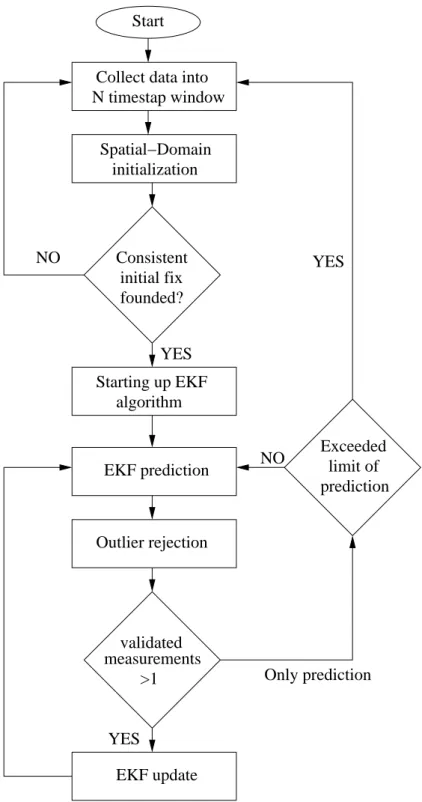
In this section two factor that afflict the EKF algorithm are discussed. The first concerns the choice of the initial point, the second concerns an on-line measurement validation. EKF is not a optimal estimator, thus with an inaccurate choice of initial point the filter may quickly diverge. On-line validation is also a critical aspect, because the estimation process of the filter depends on the past measurements, thus an outlier (completely wrong measurement) introduces significant errors in the estimation of current and future fixes. In order to run the EKF algorithm in real-world applications, the design precess has to consider also these two aspects. A spatial-domain technique is used to solve the initial position issue, instead for measurement validation a time-domain technique is presented. This approach is discussed on [2] and [30].
5.1
Initialization algorithm
Determaine a initial fix is not a trivial issue, because the presence of outliers could generate completely wrong estimates. For this reason, the initialization process cannot base the estimate only on current time; In practice, it is possible to wait for several GIB cycles before able to determine the initial fix. Moreover, the window of time considered on fix estimation has to be enough informative, thus at least three or more measurements are needed. GIB architecture gives three measurements from each buoys for timestamp. On this discussion the data received from each buoys may represent a possible combination of the following three cases: τi = di + ωi τi = di + k∆z + ωi τi = ωi
Obviously, if the range and depth information are available from one buoy in an emission cycle, the range TOA is received before the depth TOA. Assuming that at each timestamp, all the time of arrivals (GIB measurements) are less than 1000ms and at least three buoys are
Chapter 5. Initialization and Outlier rejection algorithms
working correctly, an algorithm based on least square estimation residual can be introduced. The algorithm works on windows of time, where the size is a parameter select from the user before system deployment. First, the algorithm store measurement, until the window size is reached, than start to test all possible combination of three measurements for each timestamp in the window. In a timestamp one or four estimate could be available, if three or four buoys are working respectively, other combination are wrong. Each instance of trilateration produce a fix, the quality of estimates is determine by a test on residuals. Lets define l(r) = 1 (2π)m2R 1 2 exp{−1 2(r − ˆd) TR−1 (r − ˆd)} (5.1)
where r measured ranges, ˆd estimated ranges, and
R = E{ωωT}. (5.2)
For each timestamp is selected the fix with highest probability that satisfy the following inequality
(r − ˆd)TR−1(r − ˆd) < α
1 (5.3)
where α1 is a value chose in accord with χ2 distribution (see appendix B).
After this step are available N or less candidate fixes, where N is the size of the window. The selected candidate could not represent only combination of real ranges but also combination of real ranges and outliers, in order to reject wrong fixes a χ2
test is done again. In this case is considered the trilateration error covariance and a term that consider the AUV motion capabilities is added. Lets define l(ˆpi) = 1 (2π)21|R| exp{−1 2(ˆpi− ˆpj) TΣ−1 (ˆpi− ˆpj)} (5.4)
where ˆpi and ˆpj represent the estimated fixed on timestamp i and j, h represent the sample
time, and Σ = (ATMTS−1MA)−T +V 2 M AXh 2 (i − j)2 9 I2 (5.5)
where the first term comes from (3.28) and S = 4MDRDMT. The second term is derived
from the assumption that the AUV probability of moving with a speed less than VM AX is
equal to 3σ. 3σ = VM AX (5.6) σ = VM AX 3 (5.7) σ2 = V 2 M AX 9 (5.8) 48
Chapter 5. Initialization and Outlier rejection algorithms
The factor h2
(i − j)2
in the second term of (5.5) takes in account the elapsed time between the two timestamps considered. Two estimated fixes are consistent if the following χ2
test is verified
(ˆpi− ˆpj)TΣ−1(ˆpi− ˆpj) < α2 (5.9)
The value of α2, as α1, is chosen in accord with the tabled values on appendix B. The goal
of this procedure is estimate the direction of motion of AUV and determine a reliable initial point for the tracking algorithm. The solution presented is a dedicated procedure for GIB system. Other dedicated solution for different architecture are discussed on [17] and [33].
5.2
Outlier Rejection
In the previous section the initialization issue is addressed, but another aspect have to be consider when the EKF algorithm runs. The EKF estimate depends on previous timestamps, thus if a fix estimation is afflicted by an outlier (completely wrong measurement), an error on current estimate and future estimates occurs. In order to solve this problem an on-line validation procedure is introduced. In view of the variety of variables that can be measured, a generic validation procedure for discrete-valued measurements can be introduced from the EKF theory, which is based on the measurement prediction covariance matrix.
Lets define the measurement prediction covariance matrix ([5]) Sk+1, E{˜rk+1r˜k+1T }
= Ck+1Pk+1(−)Ck+1T + 4DRDT (5.10)
where R is the measurement noise covariance matrix defined in (5.2), Pk+1(−) is the a priori
estimate error covariance matrix defined in (4.33), Ck+1 is the Jacobian defined in (4.42),
and
˜
rk+1= rk+1− ˆrk+1 (5.11)
is the innovation.
Assuming that the true measurement at time k + 1 is normally distributed, one may define a region in the measurement space where the measurement will be found with some high probability
˜
Vk+1(α3) , {˜rk+1T Sk+1−1 r˜k+1 6 α3} (5.12)
where α3 is the threshold chose in accord with the χ2 distribution (see appendix B). The
region defined by (5.12) is called the validation region. It is the ellipse of probability con-centration, measurements that lie inside the region are considered valid, those outside are discarded.
Chapter 5. Initialization and Outlier rejection algorithms Consistent founded? initial fix Spatial−Domain initialization prediction limit of Exceeded Start algorithm Starting up EKF EKF prediction Outlier rejection EKF update validated measurements >1 YES YES NO Only prediction NO YES Collect data into
N timestap window
Figure 5.1: Integration of EKF, initialization and outlier rejection procedures.