2 Nonlinear Optical Effects

2 Nonlinear Optical Effects

2.1 Fiber nonlinearities

Although nonlinear optical effects had been known as early as the nineteenth century (Pockels and Kerr effects), the field of nonlinear optics was ushered in with the development of the first laser by Maimen in 1960 [10]. This happened because lasers allow to generate light with very high intensities and these can give rise to a number of nonlinear effects.

Nonlinear behaviors come into being [1] because bond electrons start moving in an harmonic way when exposed to a strong electromagnetic field. Consequently the polarization P induced from electric dipoles becomes an electric field E nonlinear function and satisfies the more general relation:

(2.1)

(

0 : ...

P=ε χ ⋅ +E χ EE+χ _MEEE+

)

where ε0 is the vacuum permittivity, χ(j) (j=1,2,3) is the j-th order susceptibility, and ⋅, :, _M indicate tensor products.

The lowest-order nonlinear effects are originated by the third-order susceptibility χ(3), which is responsible of phenomena such as Four-Wave Mixing (FWM) and nonlinear refraction. In particular, the FWM effect concerns the generation of new frequency components.

The refractive index of the fiber becomes:

(

)

( )

2

,

n% ω E =n ω +n E2 (2.2)

where n(ω) is the linear part, |E|2 is the optical intensity inside the fiber and n2 is the nonlinear part of the index, connected to χ(3) _{by the relation:}

( )

( )

where Re stands for the real part and the optical field is assumed to be linearly polarized. Generally a nonlinear index of the fiber (the nonlinearity coefficient) is used:

2 0 eff n cA ω γ = (2.4)

with Aeff as the effective fiber core area [m2], c as the speed of light and ω0 as the central angular frequency.

The fact that the refractive index depends on the field intensity is the reason of many nonlinearities such as Self-Phase Modulation (SPM) and Cross-Phase Modulation (XPM).

2.1.1 Self and Cross-Phase Modulation

The Self-Phase Modulation (SPM) consists in a nonlinear phase modulation of a beam, caused by its own intensity via the Kerr effect. Due to the Kerr effect, high optical intensities in a medium (e.g. an optical fiber) cause a nonlinear phase delay which has the same temporal shape as the optical intensity.

If an optical pulse is transmitted through a medium, the Kerr effect causes a time-dependent phase shift according to the time-time-dependent pulse intensity. In this way, an initial unchirped optical pulse acquires a so-called chirp, i.e., a temporally varying instantaneous frequency. The total self-phase modulation contribution becomes:

( )

( )

SPM

NL z t L P teff

And the instantaneous frequency changes is (Fig. 2.1):

( )

t

ω = −∂Φ

∂ (2.6)

where P is the signal instant power, γ is the fiber nonlinear coefficient, α is the fiber loss and Leff is the effective length of the fiber:

1₋ − = z eff e L α α [m] (2.7)

Fig. 2.1: A pulse (top curve) propagating through a nonlinear medium undergoes a self-frequency shift (bottom

curve) due to self-phase modulation. The front of the pulse is shifted to lower frequencies, the back to higher frequencies. In the centre of the pulse the frequency shift is approximately linear.

.

Fig.2.2: Spectrum of an initially unchirped 1-ps pulse which has experienced strong self-phase modulation (with a

Self-phase modulation can lead to strong spectral broadening and is thus widely used in the context of nonlinear pulse compression. It is less widely known that depending on the details of the pulses, particularly their chirp, SPM can also lead to a spectral compression.

In optical fibers with anomalous dispersion, the chirp from self-phase modulation may be compensated by dispersion; this can lead to the formation of solitons. In the case of fundamental solitons, the spectral width of the pulses stays constant during propagation, despite the SPM effect.

As for SPM, it is necessary to examine Cross-Phase Modulation (XPM) as well, which is another nonlinear effect due to the dependence to the electric field intensity of the refractive index, where the intensity of one beam influences the phase change of another beam.

This effect occurs when two or more channels at different wavelengths propagate at the same time into the fiber. XPM always goes with SPM but now the phase shift depends on the fact that the refractive index is influenced by others channels power and changes from bit to bit depending on the transmitted sequence. The equation for the phase shift induced on the j-th channel is:

(2.8)

( )

( )

∑

( )

( )

( )

where N is the number of channels.

2.1.2 Four-Wave Mixing

To analytically study the Four-Wave Mixing (FWM) effect it is necessary to solve the Schrödinger equation [1] in the case that more channels are propagating on different frequencies in optical fiber.

Considering more monochromatic channels linearly polarized on the x axis and simultaneously propagating into the fiber, the total propagating field E(z,t) can be written as:

( )

{

( )

}

∑

where Ap(z) is the complex envelope of the single channel field, c.c indicates the complex conjugate terms of higher order and p is the number of channels into fiber.

The polarization state can be split in two main portion, linear and nonlinear: ( )1

_{( )}

_{( ) ( ) ( )}

( )

{

( )

}

( )

( ) ( ) ( )

∑

and the summation is extended to all the pumps (channels) whereby the relation ωi+ωj-ωk=ωf can be applied.

Analyzing all the combinations of the three indexes, it is possible to find three different contributions to the polarization state with different effects on the propagating field:

• (i=f)≠(j=k) or (i=k)≠(j=f): XPM terms due to the field at ωf and to another field at ωk≠ωf.

• (i,j)≠(k,f): FWM terms not necessary due to the field at ωf, but to fields at other frequencies for which is valid ωi+ωj-ωk=ωf.

Basically FWM is a nonlinear effect which can be observed in optical fibers when two or more fields at different frequencies propagate at the same time into fiber; this fields interact between themselves because of the nonlinear third order susceptibility effect creating new factors at new frequencies ωf. This new fields satisfy the law of conservation of energy [1]:

f i j k

ω =ω ω ω+ ± (2.16)

The interaction which origins FWM is the one that makes the relation ωi+ωj=ωk+ωf valid, where two photons annihilate themselves generating other two electrons at the frequencies ωk and ωf. The only relation that the four frequencies have

to satisfy to allow us to speak about FWM is ωi,ωj≠ωk,ωf; if that didn’t happen the nonlinearities which are generated are SPM and XPM. The FWM peculiarity is that it doesn’t necessarily depend on a signal present at the considered frequency ωf.

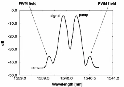
As shown in Figure 2.3, FWM also generates power at frequencies which were not filled before. Indeed at the fiber input there were only the two “pumps” (the two peaks in the center of the spectrum). It’s important to notice that the new fields can generate other fields and so on (Fig. 2.4) but the efficiency of the secondary generations is very lower, so they can be generally ignored.

Fig. 2.4: Example of FWM with generation of secondary components. Pumps wavelength were chosen nearby the

zero dispersion point of the fiber to maximize FWM efficiency.

The FWM phenomenon deteriorates an optical communication system performances in two ways: on one hand it moves part of the input signal energy on other frequencies (pump depletion) and on the other hand the moved energy can fall on frequencies where other signals are (cross-talk).

The fact that ωi could overlap with ωj suggests the following distinction between two kinds of FWM:

• ωi=ωj, partly degenerate FWM: only two pumps interact with each other to generate a third frequency ωf=2ωi-ωk. The number of possible combinations which origin new frequencies is N(N-1) where N is the number of channels. • ωi≠ωj, non degenerate FWM: the two combinations i, j, k and j, i, k origin

the same frequency ωf=ωi+ωj-ωk. The number of new frequencies generated in this case is N(N-1)(N-2)/2.

(

)

It is demonstrated [1] that the power associated to each FWM field is:

( )

( ) ( ) ( )

( )

f i j k eff

P z t ₌γ d P t P t P t e−α L z η_{ijk (2.18)}

where ηijk is the FWM efficiency:

(

)

(

)

where ∆βijk is the phase matching index among the interacting pumps.

d (degeneration element) is equal to 1 or 2 depending on the fact that the FWM case is partly degenerate or non degenerate. As a matter of fact, in the non degenerate case the two combinations i, j, k and j, i, k origin two different terms at the same frequency which are in phase with each other and which could be considered as a sole term with double amplitude; therefore their power is four time grater than the one which comes from a single term.

The effective length Leff has the goal to take into account attenuation of fields which generate FWM. If α tends to zero, Leff becomes closer to z, while for a certain value of α, the effective length tends to saturate at the value 1/α after a distance equal to 3-4 times the value of 1/α itself. Leff physical meaning is that the nonlinear effects into the fiber are all focused in the first kilometers of the propagation, whereupon the fiber conducts itself as it was a linear medium.

It is demonstrated [1] that if the channels are uniformly spaced with step ∆λ, the more efficient FWM term is the partly degenerate for which ∆λik=∆λjk=∆λ.

It is also possible to show [1] that for equally spaced channels in the case of partly degenerate behaviour it is valid:

2 2 0 2 ijk c n π β λ ⎛ ⎞ ∆ = _⎜ ∆ ⎝ λ D⎠⎟ (2.20)

where n is the order identifier of the interfering fields and D [ps/(nm km)] is the chromatic dispersion index (explained in a better way in the next paragraph).

It is also possible to underline that ηijk quickly goes down when ∆βijk grows up.

Fig. 2.5: ηijk versus ∆λ [nm] for wide values of the dispersion D with partly degenerate FWM and with

∆λik=∆λjk=∆λ.

In Figure 2.5 it is shown the efficiency graph for different values of D versus the channel spacing, where z=100 km, for partly degenerate FWM. It is possible to notice that already for 0.8 nm spacing the FWM doesn’t represent a problem exploiting standard fiber (D=17 ps/(nm km)), while with DS (Dispersion Shifted) fiber (D=0.2 ps/(nm km)) FWM efficiency is still high also for 1.8 nm spacing. At last, NZDS (Non-Zero Dispersion Shifted) fiber (D≈2 ps/(nm km)) is a good compromise between the two previous kinds of fiber.

In spite of all, it is important to underline that nonlinearities are detrimental with regard to the trasmission systems; on the contrary, in novel applications they are exploited to implement logical functions in the optical domain (as in optical samplers or optical demultiplexers, ecc.) so it is necessary to maximize the FWM efficiency because of the relationship between the new fields energy and the energy of the original signals.

Fig. 2.6: Wavelength conversion founded on FWM in optical fiber.

As shown in Figure 2.6, FWM can be used to convert a signal wavelength into a different one. In this case a pump signal interacts with the signal we want to extract and the relationship between the two frequencies is:

2

FWM p s

ω = ω − (2.21) ω

This kind of effect may occur both in optical fiber and SOA (Semiconductor Optical Amplifier), as it will be possible to understand afterwards.

2.2 Notes on solitonic pulse compression

In optics, the term “soliton” is used to refer to any optical field that doesn’t change during propagation because of a delicate balance between nonlinear and linear effects in the medium.

The solitonic pulse compression is based on a combined effect of SPM and GVD (Group Velocity Dispersion), thus to understand how this kind of compression occurs it is needful to introduce the chromatic dispersion.

Chromatic dispersion is a dielectric materials property and it manifests itself by the fact that refractive index depends on frequency. This dependency is related to the characteristic resonance frequencies at which the medium absorbs the electromagnetic radiation from electrons oscillations [1]:

( )

∑

where n(ω) is the refractive index, ωj the resonance frequency and Bj the non-dimensional intensity of the j-th resonance. Therefore the speed of the electromagnetic radiation depends on frequency in this way:

( )

_{( )}

This relation means that if a short pulse (with a broad spectrum) propagates into the fiber, it will be distorted because of the different speed of the different spectral components.

Mathematically, the dispersion effects are analyzed considering the propagation constant β [m-1]:

( )

( )

( )

c

ω

β ω = ω = ω (2.24)

where k is the wave number in vacuum: 2 k c ω π λ = = [m-1] (2.25)

Expanding the (2.24) with Taylor’s series around the operating frequency ω0:

( )

(

)

(

)

It can be demonstrated that the pulse envelope moves into the fiber at a group velocity equal to the inverse of β1 and that β2 is responsible of the pulse enlargement:

1 1 dn ng 1 n β ω ω ⎛ ⎞ = _⎜ + _⎟= = (2.28)

2 2 3 2 2 2 2 1 2 2 dn d n d d n c d d c d c d ω ω λ β ω 2₂ ω ω ω π ⎛ ⎞ = _⎜ + _⎟≅ ≅ ⎝ ⎠ λ (2.29)

where ng and vg [m s-1] are respectively the group index and the group velocity.

Fig. 2.7: Variations of the refractive index n and of the group index ng versus the wavelength for melted silica and

variations of β2 versus the wavelength in melted silica.

Rather than β2, the dispersion index D is generally used, related to β2 by:

2 1 2 2 2 d c D d c β π _β λ 2 d n d λ λ λ = = ≅ − (2.30)

Fig. 2.8: Dispersion index D versus the wavelength in a single mode fiber.

1 2 2 1 1 g g g dv d d d d v v d β β ω ω ω ⎛ ⎞ = = ⎜_⎜ ⎟_⎟= − ⎝ ⎠ (2.31)

β2 is called Group Velocity Dispersion (GVD) parameter. The wavelength range where β2>0 is called region of normal dispersion: the higher frequencies components

(blue-shifted) of a pulse propagate slower than lower frequencies components (red-shifted). When β2<0 (region of anomalous dispersion) it happens the contrary. This

second case is very interesting for investigation of nonlinearities because in this region dispersive effects and nonlinear effects can interact originating the propagation of solitonic pulses.

In the case of propagation in a situation where both SPM and GVD are significant, the Schrödinger equation cannot be simplified but it has to be solved by numerical way [1]. In general it is used the “split-step” method, in which the fiber is segmented in quite short parts where linear and nonlinear effects are alternatively considered (Fig. 2.10). Nonlinear effects Linear effects … Linear effects Nonlinear effects

Fig. 2.9: Principle scheme of “split-step” Fourier method.

Solitonic pulse compression occurs when a soliton is propagating into an optical fiber and it depends on the interaction between SPM and GVD [11].

In a fiber without losses (α=0) the SPM balances GVD, so a fundamental soliton (soliton of order N=1) can propagate itself maintaining its characteristics. If the order of the soliton is more than 1 (upper order soliton) the envelope of the pulse periodically changes while it is propagating into the fiber. In this case the compression takes place if the phase modulation generated by SPM is stronger than the one generated by dispersion.

Fig. 2.10: Solitonic pulse compression (N>1).

Looking at Figure 2.10 it is possible to understand that the pulse undergoes a red shift on the rise front, and a blue shift on the other front.

The optimum length of the fiber (zopt) corresponds to the point where the pulse duration is minimal, and we called compression factor (Fc) the ratio between the FWHM (full width at half maximum) of the compressed pulse and the one that was at the beginning of the fiber.

One of the drawbacks of this kind of compression consists in the fact that the chirp introduced by SPM turn in a pedestal or in some side tails (Fig. 2.10).

It is also demonstrated that as the soliton order grows, the optimum length of the fiber decreases and the compression factor grows up, involving an increase of the required power and the degradation of the pulse.

2.3 Semiconductor Optical Amplifier

SOAs are born as amplifier but, due to their strong nonlinear behaviours, they have found a better role realizing logical functions or switching functions which are usefull in optical transparent networks. In this way it is possible to avoid opto-electronic conversions in signal processing stages.

A SOA can be exploited as a general gain element but it also has many functional applications including e.g. optical switching and wavelength conversion [12].

Fig. 2.11: Schematic diagram of a SOA.

As shown in figure 2.11 the SOA is driven by an electrical current. The active region in the device imparts gain, via stimulated emission, to an input signal (Fig 2.12).

Fig. 2.12: Spontaneous and stimulated processes in a two level system

The output signal is accompanied by noise. This additive noise, amplified spontaneous emission (ASE), is produced by the amplification process.

SOAs are polarization sensitive. This is due to a number of factors including the geometric waveguide structure and the gain material.

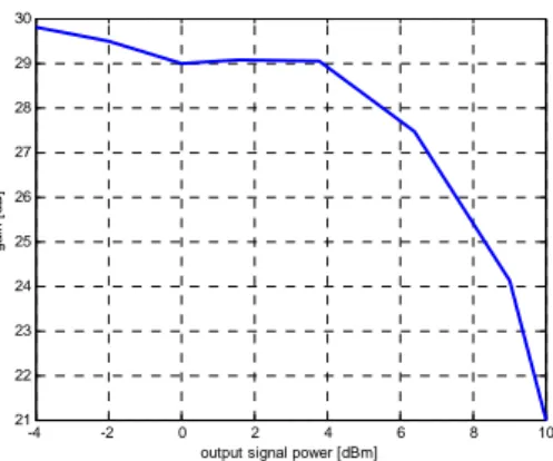
The gain of an SOA is influenced by the input signal power and internal noise generated by the amplification process. As the input signal power increases the gain decreases as shown in Figure 2.13. This gain saturation can cause significant signal

distortion. It can also limit the gain achievable when SOAs are used as multichannel amplifiers in wavelength division multiplexed (WDM) systems.

-4 -2 0 2 4 6 8 10 21 22 23 24 25 26 27 28 29 30

output signal power [dBm]

ga in [ d B ]

Fig. 2.13: SOA gain versus output signal power. This curve has been obtained through laboratory tests for a CIP SOA

with a supply current of 200mA.

SOAs are normally used to amplify modulated light signals. If the signal power is high then gain saturation will occur. This would not be a serious problem if the amplifier gain dynamics were a slow process. However in SOAs the gain dynamics are determined by the carrier recombination lifetime (few hundred picoseconds). This means that the amplifier gain will react relatively quickly to changes in the input signal power. This dynamic gain can cause signal distortion, which becomes more severe as the modulated signal bandwidth increases. These effects are even more important in multichannel systems where the dynamic gain leads to interchannel cross-talk. This is in contrast to optical fiber amplifiers, which have recombination lifetimes of the order of milliseconds leading to negligible signal distortion.

SOAs also exhibit nonlinear behaviour. These nonlinearities can cause problems such as frequency chirping and generation of intermodulation products. However, nonlinearities can also be of use in using SOAs as functional devices such as optical wavelength converters or optical logic gates.

2.3.1 Slow and fast dynamics in a Semiconductor Optical

Amplifier (interband and intraband transitions)

Supposing [13] the soa as being composed of an inhomogeneously broadened set of two-level system, it is possible to develop a theory able to describe the time behaviour of the electron and hole occupation probabilities in the conduction and valence band respectively, in the case the device works far from the steady-state condition by an injection current or an electro-magnetic field. With ρc,k(t) and ρv,k(t) the occupation probability of the k-state in the conduction and valence band is indicated. K is the wave vector that identifies the carrier momentum through the allowed conduction and valence band states, by de Broglie relation. The density matrix equations can be written as a set of differential equations where we can distinguish the processes in the conduction band[14]:

( )

( )

( )

( )

( )

( )

( )

( )

( ) ( )

and the processes in the valence band:

( )

( )

( )

( )

( )

( )

( )

( )

( ) ( )

where E(z,t) is the electric field and ρcv,k(t) is proportional to the interband polarization P(t) which takes place when an electron and a hole represent an electric dipole extremes. Λx,k indicates the equilibrium condition mutations in both the bands by the carrier pumping which due to the injection current (x=c or x=v denote respectively, the conduction or valence band). In the case that this effect occur by the E(z,t) field propagation into the guiding medium, the stimulated emissions and absorptions lead the semiconductor in a non-equilibrium state. The system aims to re-establish the Fermi distribution for the k-state, in other words the system aims to re-establish the

quasi-equilibrium condition with characteristic time τxy, and with different mechanisms depending on the type of equilibrium to be restored.

There are two different kind of equilibrium: interband and intraband. The intraband dynamics concern physical processes that change the carrier distribution in the energy space (or k-space) and redistribute these carriers within the same band. Consequently the total carrier density remains unchanged.

The first term on the right-hand side of eqq. (2.32) and (2.33) describes the relaxation of the carrier distribution function ρx,k(t), changed by external agents toward a Fermi distribution fx,k(t) due to intraband carrier-carrier scattering with characteristic time τ1x (~50fs-100fs).

The Fermi distribution describes the probability that an energy state Ex,k is occupied by a carrier:

(

)

here Ef,x is the quasi-Fermi level, Tx is the carrier temperature, and Ex,k is the carrier energy.

The second term on the right-hand side of eqq. (2.32) e (2.33) describes the equilibration of the carrier temperatures toward the lattice temperature TL due to electron-photon collision with a constant characteristic time τhx. The temperature change is generated by the stimulated emissions and absorptions of free carriers. The stimulated emission removes “cold” carriers from the conduction band states with lower energy, maintaining the distribution of the other carriers. Consequently the mean energy increases and the carrier density warm up. On the other hand the stimulated absorption transfers free carriers to the higher energy levels within the conduction band, by a carrier photon interaction. Also in this case the mean carrier temperature increases. The “hot” carrier distribution relaxes toward the lattice temperature by means of the emission of optical phonons, with a characteristic time τhx (~0.5 ps-1 ps). The Fermi

distribution function fx,kL(t) is defined by the instantaneous carrier density and the lattice temperature:

( )

The Carrier Heating (CH) phenomenon, due to Free Carrier Absorption (FCA) and Stimulated Emission (SE) as mentioned above, presents two different characteristic times. The heating process is controlled by an intraband characteristic time due to carrier-carrier scattering.

The third term accounts for relaxations toward the thermal equilibrium distribution which will be achieved in the absence of external pumping due to spontaneous radiative and nonradiative recombinations.

Finally the term proportional to E(z,t) denotes stimulated emission and absorption and Λx,k denotes pumping due to carrier injection.

Also interband phenomena affect the SOA gain. The interband phenomena, contrary to the previous phenomena modify the total carrier density within the conduction and valence band. This effect is called Carrier Density Pulsation (CDP). The injected current aims to re-stablish the dynamic equilibrium with characteristic times of few hundreds of picosecond.

In brief, when an optical field propagate into a SOA, mainly the stimulated emissions generate carrier recombination that changes both the carrier density N(t), and the temperature Tx(t) in the conduction and valence bands. Therefore the crystal equilibrium varies producing a variation of the quasi-Fermi levels and then of the Fermi distribution function. The crystal aims to re-stablish the initial equilibrium condition in the above described way: the carrier population is restored by means the injected current (interband phenomenon) and the redistribution of the carriers in the bands due to carrier-carrier and carrier-photon.

Fig. 2.14: Slow and fast dynamics in SOAs.

2.3.2 SOA nonlinearities

SOAs can also be used to perform functions that are useful in optically transparent networks. These all-optical functions can help to overcome the ‘electronic bottleneck’. This is a major limiting factor in the deployment of high-speed optical communication networks. Many of these functional applications are based on SOA nonlinearities. The development of photonic integrated circuits (PICs) has made feasible the deployment of complex SOA functional subsystems. Nonlinearities in SOAs are principally caused by carrier density changes induced by the amplifier input signals. The four main types of nonlinearity are: Cross Gain Modulation (XGM), Cross Phase Modulation (XPM), Self-Phase Modulation (SPM) and Four-Wave Mixing (FWM).

The material gain spectrum of a SOA is homogenously broadened. This means that carrier density changes in the amplifier will affect all of the input signals, so it is possible for a strong signal at one wavelength to affect the gain of a weak signal at another wavelength. This non-linear mechanism is called XGM.

Fig. 2.15: Modulation induced by XGM in SOA on a signal.

The most basic XGM scenario is shown in Figure 2.15, where a weak CW probe light and a strong pump light, with a small-signal harmonic modulation at angular frequency ω, are injected into a SOA. XGM in the amplifier will impose the pump modulation on the probe. This means that the amplifier is acting as a wavelength converter.

Fig. 2.16: Simple wavelength converter using SOA XGM.

The most useful figure of merit of the converter is the conversion efficiency, defined as the ratio between the modulation index of the output probe to the modulation index of the input pump.

The refractive index of a SOA active region is not constant but it is dependent on the carrier density and so the material gain. This implies that the phase and gain of an optical wave propagating through the amplifier are coupled via gain saturation. This strength of this coupling is related to the linewidth enhancement factor αl. Plots of αl versus photon energy are shown in Fig. 2.16.

If more than one signal is injected into an SOA, there will be cross-phase modulation (XPM) between the signals. XPM can be used to create wavelength converters and other functional devices. However, because XPM only causes phase changes, the SOA must be placed in an interferometric configuration to convert phase changes in the signals to intensity changes using constructive or destructive interference.

Fig. 2.17: Calculated linewidth enhancement factor versus wavelength for undoped InGaAsP. The parameter is

carrier density.

Four-wave mixing (FWM) is a coherent nonlinear process that can occur in an SOA between two optical fields, a strong pump at angular frequency ω0 and a weaker signal (or probe) at ω0-Ω, having the same polarization. The injected fields cause the amplifier gain to be modulated at the beat frequency Ω. This gain modulation in turn gives rise to a new field at ω0+Ω, as shown in Figure 2.17. FWM generated in SOAs can be used in many applications including wavelength converters, dispersion compensators and optical demultiplexers.