Tectonics and kinematics of curved mountain belts: examples from the Andes and the Alps

UNIVERSITÀ DEGLI STUDI DI BOLOGNA

Facoltà di Scienze Matematiche Fisiche e Naturali

Dottorato di Ricerca in Geofisica

XXI Ciclo

Settore scientifico disciplinare: GEO/10

TECTONICS AND KINEMATICS OF CURVED

MOUNTAIN BELTS: EXAMPLES FROM THE ALPS

AND THE ANDES

Ph.D. Thesis by:

Tutor:

Marco Maffione

Dr. Fabio Speranza

Co-tutor:

Dr. Rubén Somoza

Supervisor:

Prof. Claudio Faccenna

Coordinator:

PART I. INTRODUCTION TO THE CURVED MOUNTAIN BELTS...1

CHAPTER 1. General features, kinematics, and mechanisms of formation...2

1. Introduction and aim of the study...3

2. Methods...6

2.1. Paleomagnetism: potentialities and restrictions...6

2.2. Structural analysis...9

3. Brief history of the orocline concept...10

4. The oroclinal test...13

5. Different geometries of orogenic bends...18

6. Kinematics of orogenic bends...20

6.1. Marshak’s classification of kinematic patterns...20

6.1.1. Primary arcs...21

6.1.2. Secondary arcs...22

7. Mechanisms of orogenic bends formation...24

7.1. Nonrotational arcs related to “indenters”...25

7.1.1. The problem of tangential extension...27

7.1.2. The example from the Carpathian Arc...29

7.2. Nonrotational arcs formed along irregular continental margins...34

7.2.1. The example from the Appalachian (Pennsylvania, North America)...34

7.4. Basin-controlled orogenic bends...40

7.4.1. The example from the Jura Arc (Northern Alps)...42

7.5. Topography-driven arcs...45

7.5.1. The example from the Hellenic Arc...48

7.6. Orogenic arcs linked to the bending of “ribbon continent”...53

7.6.1. The example from the Great Alaskan Terrane Wreck...53

7.7. Subduction-related arcs...56

7.7.1. The example from the Calabrian Arc (southern Italy)...59

7.8. Oroclines formed by orogen-parallel compression (buckling)...63

7.8.1. The example from the Cantabria-Asturias Arc (northern Spain)...64

PART II. THE EXAMPLES FROM THE ALPS AND THE ANDES...68

CHAPTER 2. The Western Alpine Arc...69

A synchronous Alpine and Corsica-Sardinia rotation...70

1. Introduction...70

2. Tectonic setting of the Alpine-Apenninic chain in the Mediterranean domain: interplay between Africa-Eurasia convergence and Tertiary roll-back of subducting slab fragments...73

3. Previous paleomagnetic evidence from the western Alpine-northern Apennine chain, the Adria and Corsica-Sardinia (micro) plates, and the Tertiary Piedmont Basin...73

6. Results...76

6.1. Biostratigraphy...76

6.2. Magnetic mineralogy...78

6.3. Anisotropy of magnetic susceptibility...80

6.4. Paleomagnetism...80

7. Discussion...83

7.1. Local vs. uniform rotations at the TPB...83

7.2. Magnitude and timing of rotations...86

7.3. Rotation of the TPB in the frame of Alpine-Apennine tectonics...87

7.4. No paleomagnetic rotation of Adria after mid Miocene times...89

7.5. The enigmatic nature of the TPB: information from anisotropy of magnetic susceptibility data...89

7.6. The connection between Alps and the Apennines: insight into the mechanism of the Mediterranean Arc formation...90

8. Conclusions...91

References...91

CHAPTER 3. The Bolivian Orocline...95

Bending of the Bolivian orocline and growth of the Central Andean plateau: paleomagnetic and structural constraints from the Eastern Cordillera (22-24°S, NW Argentina)...96

2.1. Regional geology...100

2.2. Timing of deformation within the Eastern Cordillera and the surrounding regions...101

2.3. Previous paleomagnetic studies from the Central Andes and their tectonic implications...103

3. Geological setting of the study area...105

4. Sampling and methods...109

5. Results...110

5.1. Magnetic mineralogy...110

5.2. Paleomagnetic characteristic directions...112

5.3. Structural analysis...115

6. Discussion...122

6.1. Paleomagnetic rotation pattern from the Eastern Cordillera...122

6.2. Oroclinal test: implications for the structural style and deformation timing...126

6.3. Style and timing of deformation in the Eastern Cordillera: interplay between compressive and strike-slip tectonics...128

6.4. A southward lateral growth of the Puna plateau?...132

7. Conclusions...134

8. Acknowledgements...135

Table 1...136

CHAPTER 4. THE PATAGONIAN OROCLINE...140

Paleomagnetic evidence for a pre-early Eocene (~50 Ma) bending of the Patagonian orocline (Tierra del Fuego, Argentina): paleogeographic and tectonic implications...141

Abstract...141

1. Introduction...142

2. Background...146

2.1. Geology of the Patagonian and Fuegian Andes, and structural setting of the Magallanes belt of Tierra del Fuego...146

2.2. Previous paleomagnetic data from the Patagonian orocline and the Antarctic Peninsula...150

3. Sampling and methods...152

4. Results...154

4.1. Magnetic mineralogy...154

4.2. Anisotropy of magnetic susceptibility...156

4.3. Paleomagnetism...158

5. Discussion...161

5.1. Rotational nature of the Patagonian orocline, and relations with Scotia plate spreading and Drake Passage opening...161

5.2. Unravelling the relative relevance and timing of thrust vs. strike-slip tectonics in the Fuegian Andes: evidence from magnetic fabric...164

Table 1...169

Table 2...170

PART III. CONCLUSIONS...171

Chapter 5. Results, implications, and concluding remarks...172

1. Main results and implications from the studied curved belts...173

2. Concluding remarks about curved mountain belts and their study...175

PART I

INTRODUCTION TO CURVED

MOUNTAIN BELTS

CHAPTER 1

General features,

kinematics,

and mechanisms of formation

1. Introduction and aim of the study

Curved mountain belts have always fascinated geologists and geophysicists because of the complexities arising from their peculiar structural setting and geodynamic mechanisms of formation. Generally, during the convergence of two lithospheric plates, the mountain building process results in a relatively straight orogenic belt parallel to the plates margins. Thus, the question arises as to why curved mountain belts formed. Since the beginning of the past century, well before the plate tectonics theory was formulated,

Argand [1924] first, and Carey [1955] after, tried to explain the significance of these

great-scale curved orogenic structures, being aware of their geodynamic importance.

A huge amount of structural, paleomagnetic, seismological, analogue modelling, and geophysical studies carried out during the last 50 years, have dealt with curved orogenic belts, trying to answer to the following questions: what are the mechanisms governing orogenic bends formation? Why do they form? Do they develop under particular geological conditions? And if so, what are the most favourable conditions to their genesis? What are their relationships with deformational history of the belt? Why is the shape of arcuate orogens in many parts of the Earth so different? What are the factors controlling the shape of orogenic bends?

Relevant contributions to the understanding of the curved mountain belts have been given through time, though several aspects remain still obscure because of the geological complexities of particular orogenic domains. In fact, as we will show in this study, many factors can control arc formation, and only a detailed multidisciplinary approach, not always and everywhere possible, can contribute to the unravelling of the tectonic and geodynamic evolution of complex orogens.

Likely, arcuate structures are not uncommon features in a mountain belt, but rather a logical and simple consequence of the orogenesis. This implies that the answers to the above questions about curved mountain belts can help scientists to understand some basic (and probably not still fully understood) mechanisms of mountain building.

With this study I wish to give a little contribute to the knowledge of orogenic arc formation from different geological contexts. To reach this goal I investigated three very relevant orogenic bends: the Western Alpine Arc (NW Italy), the Bolivian Orocline (Central Andes, NW Argentina), and the Patagonian Orocline (Tierra del Fuego, south Argentina). These regions were selected because of the still open debate on the timing and kinematics of their formation. Also, the geodynamic mechanisms governing the development of bending at these regions are still subject to different, and sometimes contrasting, speculations.

I mainly used paleomagnetism, and, where possible, structural analysis, as research tools. Paleomagnetism is the unique technique able to document the deformation of a belt from the point of view of the pattern of vertical axis rotations. In fact, only paleomagnetism can document the occurrence and timing of a possible bending process. Contextually, a structural analysis was carried out to definite the strain pattern of the area, including tectonic transport directions on fault planes. Brittle fault plane directions, and relative kinematic indicators (i.e., slickensides, mineral fibers growth, SC-structures) were measured in order to unravel the features of the tectonic regime responsible of the mountain building.

I will not discuss in this work the fundamentals of these two techniques because it is out of the aim of this study, and furthermore, paleomagnetism and structural geology

analysis are two well known and extremely diffuse methods. Conversely, I will show how these tools can be properly used in the study of curved mountain belts.

The thesis is composed by three parts: parts I, II, and III. In the first part, I will show the different types of orogenic bends, their classification and kinematics, and their mechanisms of formation, reporting for each one of them a natural example from previous studies. Part II is composed by one published and two submitted papers relative to paleomagnetic investigations I carried out in three different orogens: the Alps, the Central Andes, and the Southernmost Andes. I report on paleomagnetism and structural geology of three striking orogenic bends, the Western Alpine Arc, the Bolivian Orocline, and the Patagonian Orocline, inferring tectonic and geodynamic implications for their evolution. Finally, in part III I will conjointly discuss the results of this study, also taking into account literature data, making concluding remarks about general aspects of curved mountain belts and their study.

2. Methods

2.1. Paleomagnetism: potentialities and restrictions

This paragraph does not contain presentation of the paleomagnetic technique, as it is a well known and widely diffuse method in tectonic studies. For the knowledge of fundamentals of paleomagnetism I suggest specific books, such as those by Tarling [1983],

Tauxe [1998], and Butler [2004]. On the contrary, I consider more useful showing

potentialities and limitations of paleomagnetism in the study of curved mountain belts. During the past few decades, paleomagnetism has been used as a primary tool to assess kinematic models of curved orogenic systems around the world because of its great potential in quantifying rotations along vertical axes [Carey, 1955; Eldredge et al., 1985;

Marshak, 1988; Van der Voo et al., 1997; Weil and Sussman, 2004]. On the basis of the

spatial and temporal relationships between deviations in structural trend and the vertical axis rotations observed in a given belt, it has been possible to unravel the tectonic evolution of arcuate belts. In fact, only paleomagnetic data can assess when, how, and how much different segment of an orogenic bend rotated during deformation. In the specific case of the study of curved mountain belts paleomagnetism represents the only possible technique to distinguish between different types of orogenic arcs, depending on magnitude and timing of their bending process.

On the other hand, few basic assumptions, determining together its limitations, are needed by paleomagnetism. The first assumption is that rotations in an orogenic belt occur within rigid crustal blocks separated by discontinuities (i.e., faults). In this way it is neglected the inner deformation of rocks. However, Lowrie et al. [1986] have demonstrated that in very deformed rocks paleomagnetic directions can be influenced by the local strain, resulting in spurious rotations. Thus, the applicability of the paleomagnetic

method is restricted to weakly deformed rocks in brittle deformation context. Lithology is the other great limitation in paleomagnetism: depending on the type and amount of mineral magnetic carrier content, only a limited percentage of rocks yields a stable and measurable Natural Remanent Magnetization (NRM) by which vertical axis rotations are computed. Generally, among sedimentary rocks, the most suitable lithologies are fine-grained muddy formations, while among igneous rocks, both effusive and intrusive lithologies can yield reliable results. In particular, volcanic rocks are generally characterized by a strong magnetic signal due to the high content of ferromagnetic mineral (i.e., magnetite). Finally, metamorphic rocks can record a NRM, but paleomagnetic directions suffer of strong uncertainties linked to both the age of magnetization and the lack of paleo-horizontal control needed for computing of the tectonic rotations.

With paleomagnetism we can infer tectonic rotations occurred in a given region and relate them to an accurate time interval. This can be made if two conditions are satisfied: (1) the age of the sampled rock is well known, and (2) the NRM recorded by the rock is a primary remanent magnetization. The rock age can be inferred by paleontology (in sedimentary rocks), or radiometric data (in igneous-metamorphic rocks). If the NRM constitutes a primary magnetization, then the ages of magnetization and of rock formation are coincident. In this way we can choose the correct paleopole (see Besse and Courtillot [2002]) when computing the rotation values by the paleomagnetic declinations. Then, we can correlate the computed tectonic rotations to the time interval that follows to the acquisition age of the NRM. Nevertheless, if a NRM is not a primary magnetization it is possible to infer the magnetization age relying on the knowledge of the timing of the main deformation phase.

Also, rocks sampling procedure can affect paleomagnetic results. In fact, spacing of single cores sampled within a site (or locality) should be made in order to average out the secular variation of the geomagnetic field. Because the paleosecular variation is averaged within several millennia, just a single core ~2 cm height sampled from a sedimentary formation characterized by a low sedimentation rate (i.e., 0.01 mm/a) could have recorded an averaged geomagnetic field. Yet, rock samples are commonly gathered within two 1-2 m (or more) spaced outcrops. Generally, sampling from volcanic formations, that acquire their NRM instantaneously after cooling below the blocking temperature of the main magnetic carriers, should be carried out collecting samples relative to different eruptive episodes.

A peculiar problem in paleomagnetic studies applied to tectonics is found when sampling rocks from high latitudes. Having the geomagnetic field vector a high dip value, up to 90°, magnetic declination which represent the projection of the vector onto the horizontal plane will yield a wide error bar near the geomagnetic poles. This is easy to understand looking at the equation (1) showing the declination error (ΔD):

ΔD = α95 / cos(I) (1)

Where α95 is the Fisher’s [1955] statistical parameter estimating precision of the mean

paleomagnetic direction (in degrees) on a spherical distribution, and I is the magnetic inclination, given by the projection of the geomagnetic field vector onto the vertical plane. It can be noted from equation (1) that for high values of I also the declination error (ΔD) is

high. The declination error coincides to the α95 only when the geomagnetic field vector is

horizontal (i.e., near equatorial latitude).

Finally, it should be taken into account that an intrinsic restriction to the paleomagnetic technique exists, due to natural paleomagnetic scattering, errors induced

during sampling, instrumental errors, or local magnetic anomalies. This implies that the normal resolution of paleomagnetism is about 10° in declination, as also suggested by

Lowrie and Hirt [1986], and thus rotations lower than 10° can hardly be considered as

significant.

2.2. Structural analysis

Many authors who tackled the study of curved mountain belts have evidenced the need of an integrated paleomagnetic and structural investigation [e.g., MacDonald, 1980;

Lowrie and Hirt, 1986]. In fact, paleomagnetic data should be interpreted according to the

structural framework of a given region, but, on the other hand, structural data require a paleomagnetic control. Thus, paleomagnetism and structural analysis are two complementary tools for studies in orogenic settings.

Kinematic analysis reveals to be the most useful method in structural investigations, because it can supply information on the evolutionary history of an orogenic belt. Kinematic analysis is based on the study of finite strain of a deformed area and, in particular, on the measuring of kinematic indicators on fault planes. This allows us to calculate the tectonic transport direction at a local scale, indicating the movement of the hanging wall, and, through an extensive analysis, draw the displacement trajectories path within the entire belt. Through the study of temporal and spatial variation of transport directions in orogenic arcuate systems it is possible to infer on the tectonic evolution of the bend [e.g., Nur et al., 1986; Allerton, 1994].

There are several kinematic indicators used for kinematic analysis in brittle deformation settings, but the most common and easy to recognize is represented by fault lineations (or slickensides) [Allerton, 1998]. These are represented by the growth of

elongated mineral fibers (quartz, calcite, etc.), or abrasion features originated on the fault plane during slip motion. Direction of fault lineations constitutes a strong constrain to the real displacement of the hanging wall on a fault plane. The sense of shear is usually inferred by other kinematic indicators, such as SC-structures and quartz/calcite steps.

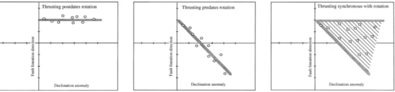
One simple and powerful tool in the analysis of rotational thrust systems involves comparison of fault lineation directions with amount of paleomagnetic rotations over a series of thrust sheets [Allerton, 1998]. Three alternative situations can be considered (Figure 2.1): (1) the thrust lineations post-date rotation. In this case a plot of lineation vs. paleomagnetic declination will show constant lineation directions for a range of declinations. (2) The thrust lineations pre-date rotation. In this case, the lineations vs. paleomagnetic declinations plot on a unitary slope line. (3) The thrust lineations are synchronous with rotation, so the lineations and declinations plot in a region bounded by a line of constant lineation, and a line with a slope of unity. The intersection of the two lines marks the true transport direction and the paleomagnetic reference direction.

Figure I 2.1. Fault lineation direction vs. paleomagnetic declination for three different cases. (left), thrust postdates rotation. (Center), thrusting predates rotation. (Right), thrusting synchronous with rotation. Modified from Allerton [1998].

3. Brief history of the orocline concept

Well before the plate tectonics theory was diffused (1960s) several ideas, sometimes contrasting, were proposed about the origin and the geologic significance of

curved mountain belts. Indicating simply geometric aspect, Miser [1932] coined the terms “salient” and “recess” to distinguish between arcuate shape orogens with curvature convex and concave toward the foreland, respectively. In this meaning, the terms salient or recess were used to indicate any curved orogenic system regardless to their kinematics and mechanisms of formation.

With the diffusion of the plate tectonics theory it was clear that the understanding of curved belts could be the key to reveal the fundaments of the orogenesis. The term “orocline” was introduced for the first time by Carey [1955] and its etymology comes from Greek and means both mountain and bend. The Carey’s definition of orocline was used to indicate an initially straight fold-thrust belt that acquired curvature during a second deformation event. However, during the following years, the term orocline have been erroneously used to indicate any curved belt, thus yielding only a geometric meaning. This was due to the concrete difficulties in inferring the timing of formation of the arc. Carey distinguished oroclines by primary bends, which, on the contrary, formed when younger orogens were molded onto the irregular margins of preexisting cratons.

The orocline concept was following redefined by Marshak [1988] who linked the term to a specific kinematics. In fact he distinguishes between oroclines, that formed by the bending of an originally linear mountain belt, and “nonrotational arcs”, which represent curved fold-thrust belts that initiate in their present curved form and their curvature does not increase during subsequent deformation. As a result, nonrotational arcs are discerned by oroclines by the fact that the formers preserve their shape during deformation, and no segment of the arc undergoes vertical axis rotations. Conversely, oroclines are characterized by opposite rotations of the limbs of the bend during its formation, according to a mechanism which is called oroclinal bending. Oroclines and nonrotational arcs have

also been called primary and secondary arcs, respectively, while the term “bend” started to be used to indicate any generic fold-thrust belt with a curved shape.

Many years later, Weil and Sussman [2004] proposed a new classification scheme

of curved belts relying on the timing relationship between thrusting and vertical axis rotations. According to this classification, nonrotational arcs and oroclines represent two end-members models among possible curved mountain belts. In nonrotational arcs, no vertical axis rotations occur and the formation of the curvature predates deformation, while in oroclines, rotations accompanying arc formation postdate thrusting. Among these, Weil

and Sussman [2004] considered an intermediate type of bend whose arcuate shape

develops contemporaneously with growth of the belt, called progressive arc. A progressive arc is defined as an orogenic belt that either acquires its curvature gradually throughout the belt’s deformation history, or a belt that acquires a portion of its curvature during a subsequent deformation phase of the belt.

Used nomenclature

In order to better understand the following discussions, I introduce some specific terms used to geometrically describe an orogenic bend [Marshak, 1988; Macedo e

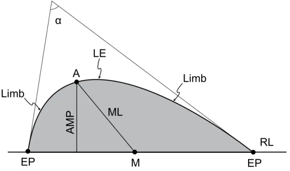
Marshak, 1999]. Figure 3.1 shows the main geometric features cited below.

The leading edge (LE) is the line that defines the boundary between the curved fold-thrust belt and the foreland basin (“marker line” in Marshak [1988]). The apex (A) is the point where the leading edge has the smallest radius of curvature. As such, the apex corresponds to the hinge point on a fold profile. The hinge zone represents the region along the leading edge, surrounding the apex. The endpoints (EP) are the points at either end of the salient at which it terminates, while the reference line (RL) constitutes the straight line

connecting the two endpoints. The limbs are the regions between the hinge zone and the endpoints. The midpoint (M) is the point halfway between the two endpoints, as measured along the reference line. The amplitude (AMP) is the shortest distance between the reference line and the apex. The midline (ML) represents the line that connects the midpoint to the apex. The interlimb angle (α) is the angle between the two legs of a triangle, in which the salient can be inscribed. The degree of asymmetry (DA) constitutes the ratio between the midline and the amplitude. It describes the inclination of the midline with respect to the amplitude, and thus can also be represented by the angle between the midline and the reference line. Finally, the area ratio (AR) is the ratio between the approximate area of the salient and the area of the interlimb triangle.

EP

RL

EP

M

ML

LE

ά

Limb

Limb

AMP

A

Figure 3.1. Simplified scheme showing the main geometric elements of orogenic bends.

4. The oroclinal test

Since the 1980s, when paleomagnetism started to be used in the study of orogenic bends [Van der Voo and Channell, 1980], it was possible to unravel the deformation

history of a curved fold-thrust belt, and distinguish between primary and secondary curves. After the first studies it became soon clear that paleomagnetism could represent a very strong constraint to the kinematics of an orogenic bend.

Paleomagnetic analysis in the study of orogenic bends is based on the fundamental principle that bending of an initially straight structure is accompanied by a variation in the direction of magnetic declinations within different sectors. Necessary condition is that the natural remanent magnetization of rocks be a primary magnetization. This variation is proportional to the deviation of the direction of the main structural features in the belt (i.e., fold axes). Conversely, in a primary arc, the direction of magnetic declinations does not change along the entire arc.

Yet, some studies have documented intermediate paleomagnetic directions with respect to those expected, according to the structural deviation observed in the belt [Bachtadse and Van der Voo, 1986; Miller and Kent, 1986]. This could imply an oroclinal bending of an already partially curved belt. But, how can we quantify the real correlation between paleomagnetic and structural directions? Opposite vertical axis rotations within the limb of a curved orogenic belt, in fact, do not necessarily indicate that it represent an orocline.

Commonly, two analogueous statistical tests (oroclinal test) are used in order to estimate the degree of correlation between paleomagnetic and structural directions in a curved fold-thrust belt. In the first test, proposed by Schwartz and Van der Voo [1983] a linear regression is performed on a data population plotted in an orthogonal diagram where the X and Y coordinate for each point is represented by the difference between the local

strata direction (S) and the mean value of the strata directions (S0), and the difference

(Figure 4.1). In the second test, proposed by Eldredge et al. [1985], the X and Y coordinate of each point from data population is given by the difference between the reference

structural direction (Sr) (considered as the initial direction of the orogen before bending)

and local strike of fold axes (So), and the difference between a reference declination value

(Dr) (which is generally the declination value from the foreland area) and the site mean

declination (D) (Figure 4.2).

An essential condition is that rocks used for an oroclinal test must have a similar

age, otherwise, different reference declinations (Dr) should be considered for each group of

sites with similar age. Conversely, the choice of the reference declination for similar age rocks does not influence the result of the test.

S-S₀

D-D_{0 Regression line}

D_r-D

S_r-S

Regression line

Figure 4.2. Oroclinal test according to the method by Eldredge et al. [1985].

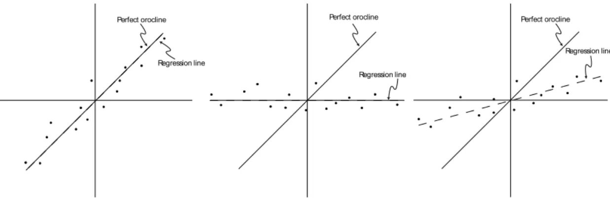
Results from the linear regression can show three end-member situations, depending on its angular coefficient (m) (Figure 4.3):

a) (m = 1): paleomagnetic declinations are 1:1 correlated with structural

directions, and the orogenic bend represents a perfect orocline.

b) (m = 0): declination values are constant over the curvature and there is no

correlation between paleomagnetic and structural directions. The bend is a primary feature and represents a nonrotational arc.

c) (0 < m < 1): variation of paleomagnetic directions is lower than variation of

structural directions. This means that the orogenic bend, formed originally curved (as a primary arc), was bent during following tectonic events.

Regression line Perfect orocline Regression line Perfect orocline Regression line Perfect orocline

Figure 4.3. Sketch showing possible results from the oroclinal test, indicating a perfect orocline (left), a primary arc (center), and a primary arc subsequently affected by some amount of oroclinal bending, or a progressive arc (right).

At this point, the statistical significance of the slope of the regression line must be quantitatively estimated comparing it with the zero or the unitary slope line. In the first works by Schawartz and Van der Voo [1983] and Eldredge et al. [1985] the correlation coefficient (C) was considered in order to estimate the significance of the linear regression. Yet, this estimate was usually very subjective, and a coefficient major than 0.8 was always considered indicative for a reliable correlation of data. After few years, a more objective tool was proposed for oroclinal tests: the statistical test [Lowrie and Hirt, 1986]. The t-test is used to assess if the slope of the regression line calculated by linear regression is statistically different from a give slope, which can be zero or one if we consider the end-member situations for a perfect orocline or a nonrotational arc. The value of t is given by the following equation:

(

)

₍

₍

(

₎

)

₎

∑

∑

- (m) is the relative angular coefficient of the regression line with respect to the reference slope. In example, for a regression line with an angular coefficient of 0.2 the

value m in the equation (1) is equal to 0.2 when compared to the zero slope line, but it is equal to 0.8 (1-0.2=0.8) if compared to the unitary slope line;

- (N) is the number of observations (data);

- (So) and (SR) are the observed and reference local structural directions, respectively;

- (Do) and (DR) are the observed and reference declination, respectively;

- (DP) is given by the following equation (2):

Dp= m (So-Sr) + c (2)

where, m and c are the parameters of the regression line.

Result from equation (1) is then compared with critical values of t depending on the value of N and the confidence (or significance) level we choose. Usually, confidence levels of 5% and 1% are used. If the t value resulted by the oroclinal test is lower than the critical value, then the regression line and the reference line are not statistically different.

So, in an ideal case where our regression line is close (but not coincident) to the zero slope line, the t-test is used to define if some oroclinal bending occurred or not.

5. Different geometries of orogenic bends

Curved mountain belts from different part of the Earth show a great variability in their geometric features, such as amplitude (AMP), interlimb angle (α), degree of asymmetry (DA) (Figure 5.1), and pattern of structural trend-line (Figure 5.2).

Figure 5.2. Types of structural trend-line patterns observed in salients. The continuous curved line represents the leading edge of the salient, whereas the broken lines represent structural trend lines. The straight line represents the reference line, and the inverted triangles define the end points of the curve. (A) Parallel trend-line pattern. (B) Convergent trend-line pattern with trend lines converging to both end points. (C) Convergent trend-line pattern with trend lines converging to one end point. (D) Divergent trend-line pattern. (E) Truncated trend-line pattern. (F) Chaotic trend-line pattern. After

Macedo and Marshak [1999].

Besides these substantial differences, several studies have demonstrated that both primary and secondary arcs can show identical final geometric features. For that reason, factors or boundary conditions common to both types of bends should exist and be independent from the mechanisms of arc formation. This consideration, once again, stresses the importance of a multidisciplinary approach (paleomagnetic and structural) in the study of the orogenic bends.

Macedo e Marshak [1999] proposed a preliminary classification for different bend

geometries based on the degree of asymmetry, dividing most of the existing curved structures into three main groups: symmetric, asymmetric, and irregular arcs. In symmetric arcs, the Amplitude (AMP) coincides with the Midline (ML), while in an asymmetric arc they form an angle which increases as the degree of asymmetry increases. In irregular arcs the Leading Edge (LE) can form small-scale secondary bends. The authors, after having checked most of the existing orogenic bends, concluded affirming that asymmetric arcs are the most frequent structures.

In the following sections the possible factors/boundary conditions controlling the final shape of an orogenic bend will be discuss.

6. Kinematics of orogenic bends

The first intuitive interpretations of arcuate fold belts consisted in “virgations du premier genre” [e.g., Argand, 1924] and were interpreted to be characterized by fanning transport directions. However, although widely diffused, orogenic bends are still not fully understood from the point of view of their kinematics. Usually, a geologist who studies an orogenic belt has to resolve an inverse problem, which is unravelling its kinematics starting from an observed finite strain. This can be made through structural analysis, and in particular with kinematic analysis on fault planes, the study of balanced cross sections, and with paleomagnetism.

During the evolution of an orogenic bend in a brittle tectonic setting, depending on the mechanism governing its formation and, thus, the type of bend (primary or secondary), individual points within the belt can show different displacement path trajectories. The first classification of kinematic patterns in curved fold-thrust belt was proposed by Marshak [1988] who demonstrated that a number of different kinematics can lead to the development of primary and secondary arcs.

6.1. Marshak’s classification of kinematic patterns

Marshak’s [1988] classification relies on 14 different kinematic patterns

characterizing both primary and secondary arcs. The evolution of an orogenic bend can be described through: (1) the displacement paths, (2) the amount and variation of the arc-parallel extension, (3) the displacement of the endpoints, and (4) the movement of the reference line.

In the next paragraph I will discuss the possible kinematic patterns for primary and secondary arcs.

6.1.1. Primary arcs

Nonrotational arcs are bends in which the strike of a segment of the fold-thrust belt does not change during the formation of the arc. Three distinct displacement path trajectory patterns can lead to the development of a nonrotational arc, such as (Figure 6.1.1.1):

- Pattern AA: the displacement path trajectories have zero length, the leading edge is fixed in position with respect to adjacent crust, and no horizontal translation occurs. Such a pattern would be characteristic of primary bends that have been subjected only to vertical movement.

- Pattern AB: the displacement path trajectories along the length of the bend are equal in magnitude and are parallel to one another. For such bends there is no tangential extension, no rotation of segments of the orogen, and no change in the curvature of the belt during its evolution.

- Pattern AC/AD: the displacement path trajectories are nearly orthogonal (AC) or orthogonal (AD) to the trend of the orogenic belt and are unequal in length. Different segments of the belt do not change strike as they translate into the foreland, while tangential extension, of variable amount along the arc, must occur during the evolution of the orogen.

AA AB AC - AD

Figure 6.1.1.1. Sketch displaying displacement path trajectory patterns for nonrotational arcs.

In the following paragraph we will show that patterns AA and AB have never been recognized in primary arcs, whereas pattern AC-AD were found to be the most diffused in nature, and a common results in numerous analogue experiments [e.g. Zweigel, 1998].

6.1.2. Secondary arcs

If the orientation or magnitude of displacement path trajectories varies around a bend in such a way that the segments of the bend change strike with time, then the bend is an orocline. The possible kinematic patterns are (Figure 6.1.2.1):

- Pattern OA: as the leading edge moves into the foreland, the bend remains a segment of a circle with the same radius of curvature. The endpoints are not fixed and there is tangential extension. The displacement path trajectories are straight lines forming a diverging fan.

- Pattern OB: the displacement path trajectories are perpendicular to the strike of the belt but vary in length around the arc. The endpoints translate into the foreland during deformation and tangential extension varies along the length of the bend.

- Pattern OC: the endpoints are fixed and the leading edge undergoes uniform tangential extension. The displacement path trajectories form a diverging fan and decrease in length toward the endpoints.

- Pattern OD: the displacement path trajectories are parallel to one another but their lengths vary continuously and decrease toward the endpoints. There must be tangential extension, but it is not uniform along the length of the arc. Endpoints are fixed.

- Pattern OE: the positions of the endpoints are fixed and no tangential extension occurs. In this case, rock must slide or flow past the endpoints. The displacement path trajectories define a convergent fan.

- Pattern OF: as the leading edge migrates into the foreland the endpoints approach one another along the reference line.

- Pattern OG: the displacement path trajectories are approximately perpendicular to the trend of the orogen and decrease in length toward the crest. Therefore the curvature of the orogen in plan view decreases as it propagates into the foreland. There is tangential extension.

- Pattern OH: one endpoint is fixed and no tangential extension occurs during development of the bend. The development of the bend involves rotation around a single vertical axis located at some point along the orogen, and the displacement path trajectories are segments of circular arcs. There is no tangential extension. A variation to this pattern is that the displacement path trajectories are parallel to one another, and perpendicular to the reference line.

7. Mechanisms of orogenic bends formation

Hitherto, the most representative geometries and kinematic patterns of curved belts have been exposed. But, the occurrence of bending in a fold-thrust belt and its main features depend on the geodynamic processes controlling their developing. As I have already said previously, paleomagnetic, structural, and geophysical data should be integrated in order to document the geodynamic framework of a curved belt, and unravel its formation mechanisms.

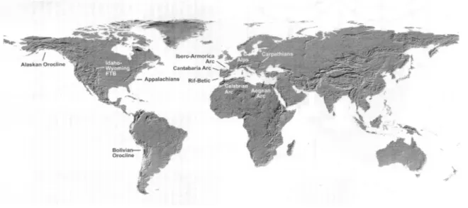
Numerous orogens in the Earth show arcuate systems (Figure 7.1). Numerous geologic factors that can control the developing of a bend exist, such as: geologic and mechanical features of the orogenic wedge and the foreland, the original shape of the sedimentary basin before deformation, the geometry and kinematic of the subducting slab, the shape of continental margins before the collision, and the presence of obstacles (or buttress), among many others.

In the next paragraphs the main orogenic bend formation mechanisms will be discussed, reporting, for each one of them, a natural example.

7.1. Nonrotational arcs related to “indenters”

The term “indenter” has been used in the past to indicate any rigid block that can collide with a continental margin. In nature, an indenter can be represented by a continental promontory or an exotic terrane (i.e., island arcs, or microplates). The effects of the convergence of indenters into a deformable material have been documented by numerous analogue experiments performed during the last two decades [Tapponnier et al., 1982;

Davy and Cobbold, 1988; Marshak, 1988; Marshak et al., 1992; Lu and Malavieille, 1994; Macedo and Marshak, 1999; Zweigel, 1998; Costa e Speranza, 2003].

The main result from these experiments is that nappes, created in front of an indenter, have curved thrust traces and fold axes in map view. Marshak et al. [1992] demonstrated that a spoon-shaped detachment surface forms following to indentation, determining the development of an initially curved structure in the hanging wall. The detachment surface has low inclination in the frontal part and becomes subvertical near the lateral edges of the indenter. During the initial phase of convergence, the displacement path trajectories in the deformed wedge show divergent fanning directions that are suborthogonal to the strike of the fold axes. In the following phase, when indentation prosecutes, a new detachment surface forms in front of the former one, and a new curved nappe develops. The displacement path trajectories in the first developed nappe are now parallel to one another, being the internal region uniformly transported toward the foreland, whereas the frontal part of the bend shows again divergent fanning displacement path trajectories.

Similar results have been documented by Costa and Speranza [2003], who performed a “magnetized analogue experiment” using sand mixed with magnetite-dominated powder. Before deformation, the model was magnetized by means of two

permanent magnets generating a quasi-linear magnetic field. After deformation, cylindrical specimens were sampled within thrust sheets, and vertical axis rotations were calculated. Their results indicate that an indenter pushing into deforming belts generally forms nonrotational curved outer fronts, while the more internal fronts show oroclinal-type rotations. This would represent a composite curved belt consisting of an orocline in the inner part and a nonrotational arc in the outer one. According to the new classification of orogenic bends by Weil and Sussman [2004], the bend formed in the inner part of the deforming wedge would represent a progressive arc, rather than an orocline.

Many analogue experiments have demonstrated that material deformed in front of the central part of the indenter is characterized by pure shear, while simple shear affects material located near its corners. This implies that the frontal part of arcs formed by indentation of a rigid block is also affected by a different amount of tangential extension (the extension parallel to the strike). The topic of tangential extension will be treated more in detail in paragraph 7.1.1. Conversely, at two limbs of the bend, clockwise and counterclockwise vertical axis rotations occur in front of the right and left corner of the indenter, respectively. Rotations are induced by internal deformation of the rock, without implying a rotation of the thrust surfaces [e.g., Zweigel, 1998]. In fact, rotation amount occurring within these portions of the bend is always minor than the structural trend variation within the arc. Therefore, the angle between a trend line and the reference line of the salient does not necessarily indicate the amount of rotation of a limb.

Zweigel [1998] suggested that several features of indenter-related bends are

controlled by the indentation angle (i.e., the angle between the indentation direction and the normal to the frontal face of the indenter). Zweigel observed that: (a) the ratio between the widths of the lateral and frontal parts of the wedge increases linearly with increasing

indentation angle, thus influencing on the final shape of the bend. (b) Tangential extension in the corner area decreases with increasing indentation angle. (c) Tangential extension in the corner area is initially high, decreases during progressive convergence, and attains a stable level during the advanced stages of the experiments when self-similarity conditions are reached. (d) Displacement vectors of accreted material exhibit fanning around the arc, but in oblique indentation the spread of their orientation is smaller than the change of structural strike (nappe traces and fold axes). In fact, displacement vectors trend mainly orthogonal to the structural grain of the belt when indentation is parallel, conversely, they rotate clockwise and counterclockwise in the left and right limb of the arc, respectively, when convergence is oblique.

Analogue experiments have also demonstrated that the final shape of the bend is controlled by different factors, such as the shape of the indenter and the shape of the sedimentary basin over which the curved structure develops [Macedo and Marshak, 1999]. The shape of the salient leading edge closely reflects the shape of the indenter: a rectangular-shaped indenter yields a flat-crested salient, a symmetric parabolic-shaped indenter yields a parabolic salient, and an asymmetric rounded indenter yields an asymmetric salient. Furthermore, these authors proposed that a salient, formed by indentation of a rigid block, can be recognized by a divergent structural trend-line pattern (see paragraph 5).

In conclusion, it can be asserted that the indentation of a rigid block within a deformable material generally produces primary arcs.

Kinematic models proposed by Marshak [1988] have evidenced that tangential extension can affect both primary and secondary arcs, though it is not a necessary consequence of bend development. The origin of the arc-parallel stretching is different in the two types of bend: in primary arcs, it is mainly associated to the pure shear generated in front of the central part of the indenter, whereas in oroclines tangential extension results as a consequence of the increasing in the curvature radius of the outer part of the arc with respect to the inner part. In examples, in oroclinal bending due to buckling, the outer and inner part of the bend undergoes arc-parallel extension and compression, respectively.

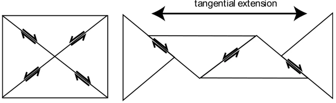
Nevertheless, how tangential extension occur in curved belts is not still fully understood. Marshak [1988], proposed two types of fracture arrays accommodating tangential extension: a multiple set of nonparallel fractures and a single parallel array. The first type has been recognized by Marshak et al. [1982] in the northern Apennines (Italy), where a widespread array of mesoscopic strike-slip faults, which roughly define a conjugate system, permitted arc-parallel extension, without implying a rotation of mesoscopic-scale blocks (Figure 7.1.1.1).

tangential extension

Figure 7.1.1.1. Sketch showing kinematics for tangential extension through a non-parallel fault array.

However, conjugate fault arrays associated to tangential extension need, not always involve strike-slip faults. For example, Ramsay [1981] documented the occurrence of tangential extension in the Helvetic nappes accommodated by conjugate normal faulting.

The second type of fracture array has been documented from the Makran Mountains (Pakistan) by Marshak [1988] and consists on a set of parallel faults produced in a region characterized by simple shear in a direction parallel to the transport direction of the belt.

7.1.2. The example from the Carpathian Arc

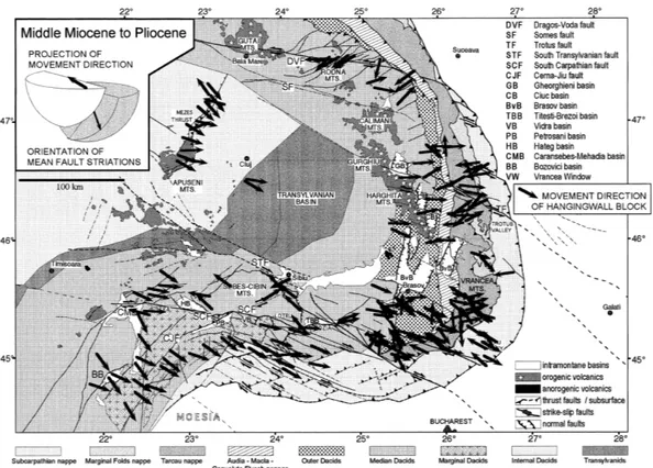
The Carpathians represent a 700-km long fold-thrust belt with a striking curved structure formed during the Late Cenozoic by the convergence of the Adriatic microplate and other continental fragments (such as the Tisia-Dacia block), with respect to Europe [Burchfiel, 1980]. The Carpathians are divided into an inner part, consisting of crystalline basement nappes and their Mesozoic sedimentary cover (Tisia-Dacia block, Inner Carpathians), and an outer part of Cretaceous to Tertiary flysch and molasse nappes (Outer Carpathians). The Outer Carpathians form a continuous, curved belt from the Western Carpathians to the southern end of the Eastern Carpathians, and continue below the Miocene to Recent sedimentary cover along the front of the Southern Carpathians (Figure 7.1.2.1).

Structures are convex towards the foreland and show outward tectonic vergence. In the Western Carpathians the orogen grain strikes ~NE-SW, then it makes curves of ~90° showing, in the Eastern Carpathians, a general NNW-SSE trending, and finally it changes to a roughly E-W direction in the Southern Carpathians [Morely, 1986; Linzer et al., 1998;

Zweigel, 1998]. The hinterland of the orogenic belt, consisting of basement units which

underwent their major deformation in the early Cretaceous (145-99 Ma) together with an accretionary wedge, exhibits a convex right-angled corner and constitutes the Tisia-Dacia block.

Figure 7.1.2.1. Geological map of the Carpathians arc system. After Zweigel et al. [1998].

Thrusts transport directions, inferred by fault lineations, exhibit a fanning distribution around the arc (Figure 7.1.2.2) [Linzer et al., 1998], and their spread is systematically smaller than the change of strike of fold-thrust structures [Zweigel et al., 1998]. According to these evidence, convergence in the Eastern Carpathians is almost normal to orogenic strike, whereas movements in the Southern Carpathians are almost pure right-lateral strike-slip to the west and right-lateral transpressive to the east [Ratschbacher

et al., 1993; Morley, 1996; Zweigel, 1997; Linzer et al., 1998]. This model is in agreement

with the increasing shortening components normal to orogenic strike of the Southern Carpathians from west to east documented by Maţenco et al. [1997].

Figure 7.1.2.2. Pleistocene to Holocene displacement orientations of hanging wall block of Eastern and Southern Carpathians. After Linzer et al., 1998.

Paleomagnetic and structural data from the Tisia-Dacia block show that the hinterland did not move straight, but carried out a clockwise rotation [Ratschbacher et al., 1993; Pătraşcu et al., 1994] followed by a small southeastward translation [Zweigel, 1997]. This rotation, resulted in an oblique indentation of the Tisia-Dacia block with the Eastern Carpathians, which is maximum (36°) in the region connecting Eastern and Southern Carpathians (Bend Area) (Figure 7.1.2.3).

Previous paleomagnetic data from the Carpathians evidenced over 90° opposite rotation on both the limbs of the arc, showing the existence of two distinctive tectonic domains: the northwestern Carpatho–Pannonian domain with systematic counterclockwise rotations and the southeastern Carpatho–Pannonian domain with systematic clockwise rotations [e.g., Balla, 1987; Linzer, 1996; Csontos and Voros, 2004; Dupont-Nivet et al.,

Figure 7.1.2.3. Clockwise rotation of the Tisia-Dacia block around a pole situated in its vicinity in western Moesia (Romania). Angles of convergence relative to the normal to strike of the orogen are shown. After Zweigel [1998].

Dupont-Nivet et al. [2005] showed that no significant rotation has affected the

eastern Carpathians since ~9 Ma. In the southern Carpathians, a ~30° clockwise rotation seems to have occurred during the 13-6 Ma time interval. This indicates that a regional tectonic event occurred in this region probably between 13 and 9 Ma.

Further (but less reliable) paleomagnetic data from Cretaceous rocks [Bazhenov et

al., 1993] would represent evidence for an early phase of clockwise rotation of 60-100° in

Southern Carpathians and 10-50° in Eastern Carpathians.

The development of the Carpathian Arc occurred during Late Cretaceous to Eocene times, when the northwestward movement of the Adriatic plate closed the Penninic oceanic basins. The Tisza–Dacia block was situated in its pre-rotational position SW of the Moesian plate (Romania). During Paleogene times, the Alpine–Carpathian orogenic front moved to the north driven by slab roll back of the oceanic lithosphere [Balla, 1987; Linzer

et al., 1998]. The Tisia–Dacia block rotated clockwise between 90º and 120º around the

Moesian plate from Late Cretaceous to Middle Miocene times, with main rotation occurring in post-Aquitanian times (<22 Ma). Dupont-Nivet et al. [2005] proposed a 30°–

span. Subsequently, the Middle Miocene to Pliocene deformation was mainly driven by retreat of the subducting slab in the embayment between the Moesian and European plates, and by the eastward escape of the Tisza–Dacia block [Ratschbacher et al., 1993]. Closure of the oceanic embayment and subsequent collision of the Tisza–Dacia block (which acted as an indenter) with the Eastern European and Moesian foreland generated the arc structure of the Carpathians, inducing a further ~30° clockwise rotation in the southern Carpathians [Dupont-Nivet et al., 2005].

Structural data indicate an Early to Middle Miocene E–W contraction, followed by Middle to Late Miocene right–lateral oblique convergence in the southern Carpathians and frontal convergence in the eastern Carpathians [Morley, 1996; Linzer et al., 1998; Zweigel

et al, 1998]. Dupont-Nivet et al. [2005] interpreted the Middle to Late Miocene vertical

axis rotations in the Eastern and Southern Carpathians as the result of the indenting of the Tisia-Dacia block within the European margin. A possible mechanism explaining the clockwise rotations in the Southern Carpathians is dextral wrench tectonics affecting this region [Linzer et al., 1998].

The early evolutionary phase of the Carpathians has been clearly controlled by retreat of the subducting slab. Conversely, the final shape of the arc appears to be a primary feature caused by the rotational indentation of the Tisia-Dacia block. The low amount (<20%) of orogen-parallel extension in the Eastern Carpathian arc documented by

Zweigel et al. [1998], constitutes a proof for the syn-accretionary character of the arc, in

contrast to secondary arcs which would require a major orogen-parallel extension [Marshak et al., 1992; Zweigel, 1997]. In turn, the movement of the Tisia–Dacia block was attributed to the pull from its front (east) due to the retreating of the subducting slab [e.g.,

Royden, 1993]. Furthermore, the fanning distribution of transport directions is a feature

compatible with results obtained from many indentation experiments [e.g., Zweigel, 1998].

7.2. Nonrotational arcs formed along irregular continental margins

Generally, if a straight continental margin is subjected to a uniform compressive stress along strike, a roughly linear fold-thrust belt develops. However, most continental margins are not straight due to many factors linked to their past evolutionary history. The shape of passive margins would determine the distribution of stratigraphic units which could in turn affect the initial geometry of thrust faults. If thrust faults are initially spoon-shaped, then the hanging wall structures will be curved in plan view and the orogen will initiate as a nonrotational arc. Being the kinematics of such structures similar to those for indenter-related primary bends, the displacement path trajectory patterns could correspond to the patterns AB or AC of Marshak’s [1988] classification (see paragraph 6.1.1).

One of the most commonly cited examples of nonrotational arcs formed as a consequence of the irregularity of continental margins is the Pennsylvania salient.

7.2.1. The example from the Appalachian (Pennsylvania, North America)

Paleozoic rocks within the central Appalachians consist of a nearly continuous section of carbonate and clastic sedimentary rocks deposited on a rifted margin of metamorphic basement [Thomas, 1977]. The Pennsylvania salient of the Valley and Ridge is composed of three roughly linear segments of different trend: a southern (020°–025°), central (055°–060°), and northern segment (065°–085°) (Figure 7.2.1.1). The culmination in the central segment (Juniata Culmination) reflects differences in map scale shortening in

the salient. In fact, rocks have been shortened 30-38% in the south, 38-39% in the north, and ~46% in the central salient [Gray e Stamatakos, 1997].

Figure I 7.2.1.1. Digital elevation model of the Pennsylvania salient showing the main physiographic features.

Regional shortening directions record as much as 30° clockwise rotation in the northern segment [Gray and Mitra, 1993] and opposite rotation sense in the southern segment [Evans, 1994]. The regional shortening directions on both limbs of the salient were initially subparallel and trended 320°–340°. After the early deformation phase which yielded a layer-parallel shortening, the shortening directions began to diverge. The final stages of deformation exhibit maximum shortening directions of 280°–290° in the southern segment, and 010° in the northern segment [Gray e Stamatakos, 1997].

Paleomagnetic results from previous studies [Schwartz and Van der Voo, 1983;

temporal relationships of deformation: (1) Folding in the salient occurred in the Permian. (2) Either prior to or during the earliest stages of deformation, rocks within the salient were rotated about a vertical axis between 20° and 30°. It remains unclear whether all of the rotation took place on one limb of the salient or whether the rotations were evenly distributed on the limbs of the salient. If both limbs of the salient rotated to achieve the overall 30° tightening of the salient, each limb must have rotated 15° in opposite directions during the earliest phase of the orogenesis. (3) Since the onset of folding and thrusting, vertical axis rotations around the salient have been negligible. Compatibly, oroclinal test performed by Schwartz and Van der Voo [1983] evidenced that paleomagnetic and structural direction are not correlated, as the best-fit line is not statistically different from zero slope line (see paragraph 4).

This implies that, despite evidence for early vertical axis rotations, curvature is an original feature of the arc. This conclusion is subsequently supported by the shortening directions that rotated in opposite sense to those predicted for an orocline, and precludes tectonic models that explain the curvature of the orogen solely in terms of impact by rigid indenters on the opposing African margin [e.g., Faure et al., 1996].

According to the tectonic model by Gray e Stamatakos [1997], lateral differences in the amount of layer-parallel shortening in the lower thrust sheet produced vertical axis rotations in the upper thrust sheet. Imbrication of the lens-shaped lower sheet eventually led to the development of a three-dimensionally tapered wedge. Gravitational spreading of the tapered wedge generated progressively radiating paleostress trajectories (and concordant maximum shortening directions within the wedge) while it inhibited further vertical axis rock rotations.

7.3. Salients associated with obstacles

An obstacle is a feature which impedes movement on a detachment fault in a fold-thrust belt. In literature, obstacles have also been indicated by the term “buttress” [e.g.,

Horberg et al., 1949]. Geologically, an obstacle can be represented by a stratigraphic

pinch- out of a glide horizon [Laubsher, 1972], a basement massif on the underthrust plate [Grubbs and Van der Voo, 1976; Schwartz e Van der Voo, 1984], a seamount or an oceanic ridge upon a subducting slab, or rigid carbonate shelf [Costa and Speranza, 2003].

If a segment of a fold-thrust belt is pinned at an obstacle while adjacent segment are able to advance, a bend may develop. The obstacle causes systematic reorientation of stress trajectories which leads to along-strike variations in displacement path trajectories [Laubsher, 1972; Beutner, 1977]. Marshak [1988] suggested that oroclines can form in association with buttresses, displaying kinematic patterns OA, OB, OC, or OD (see paragraph 6.1.2).

In the experiments by Macedo and Marshak [1999] it has been observed that when the thrust front reach the obstacles, new thrusts that form to the foreland of the obstacles initiate with a curved trace, thus yielding nonrotational arcs. Preexisting thrusts eventually undergo oroclinal bending as they force through the space between the obstacles. These authors also noted that the shape of the salient depends on the spacing between buttresses: for a given amount of shortening, the degree of curve protrusion decreases as the distance between buttresses increases. Similar results were also obtained from magnetized analogue models by Costa and Speranza [2003]. Furthermore, the relative amount of shortening, as manifested by the number of thrusts and by the thickness of the thrust wedge, is greater near the end points (EP, see paragraph 3) than near the apex.

Costa and Speranza [2003] carried out analogue experiments using different

boundary condition for buttress, such as the presence or not of a lateral confinement, the buttress type (surmontable or insurmontable in order to reproduce shallow and deep portions of the deforming sheets, respectively), and its orientation with respect to the shortening direction. Interesting aspects resulting by these experiments are listed below:

(a) Deforming wedges colliding with obstacles in the foreland, oblique to the shortening direction, display rotations of the outer fronts opposite in sign to the oroclinal rotations.

(b) The more internal fronts rotate only later, due to both lateral shear strain and interaction with later and more external fronts. They show oroclinal rotations, but the magnitude of rotation is smaller than that expected for a perfect orocline, except for those fronts formed inside the lateral symmetrical obstacles.

(c) When deforming wedges collide with obstacles, rotations more strongly affect laterally unconfined wedges. Also in thin-skinned tectonics of natural settings rotations are probably easier where rocks are poorly confined laterally or in the shallower structural levels.

In the next paragraph I will report on a natural example of arcuate belt formed in association with a buttress: the Gela nappe of the Maghrebian thrust belt of Sicily (Italy).

7.3.1. The example from the Maghrebian thrust belt of Sicily (Italy)

The Gela Nappe is a striking, southward-verging, salient corresponding to the largest southward advancement of the Sicilian Maghrebian belt over the African foreland (Figure 7.3.1.1). It is formed by a thin-skinned wedge exposing upper Miocene-mid Pleistocene basinal sediments [Lickorish et al., 1999] deformed until mid Pleistocene

times. The Gela Nappe salient develops between two uplifted domains exposing thick and rigid shelf carbonates: the Hyblean plateau to the east, and the Saccense ridges to the west.

Figure 7.3.1.1. Schematic map of Sicily and paleomagnetic orogenic rotations, after Speranza et al. [2003]. Vertical arrows indicate unrotated areas. Circular arrows (and the enclosed angle) indicate the amount of clockwise and counterclockwise rotations calculated for the single sampling localities.

Paleomagnetic studies have shown that in Sicily large-scale clockwise rotations occurred synchronous with thrust sheet emplacement [Channell et al., 1990; Speranza et

al., 1999, 2003]. Clockwise rotations seem to have a regional character, and to be

genetically related with the spreading of the southern Tyrrhenian Sea, which induced the formation of a large-scale orocline represented by southern Apennines, Calabria, and Sicilian Magherbides belt fragments [e.g., Gattacceca and Speranza, 2002; Speranza et al., 2003]. In Sicily, Speranza et al. (2003) have shown that a 70° clockwise rotation occurred in mid Miocene times, followed by a late Miocene-Pleistocene 30° clockwise rotation.

Plio-Pleistocene sediments sampled in several parts of the Gela Nappe show invariantly 10–30° CW rotations [Speranza et al., 1999, 2003]. Older pre-orogenic sediments exposed at the edges of the Gela Nappe itself similarly show a ubiquitous 100° total orogenic rotation, without any major difference between the eastern and western limbs of the salient [Channell et al., 1990; Speranza et al., 2003].

The paleomagnetic data summarized above show that the Gela Nappe salient is an almost perfect nonrotational arc, once the uniform CW rotation of the Sicilian nappes is eliminated. The two platform carbonate domes represented by the Hyblean plateau to the east, and the Saccense ridges to the west, may have represented the foreland obstacles colliding with a southward propagating thrust wedge and causing the formation of a pronounced belt salient. This hypothesis appears to be in good agreement with the results of analogue models by Costa and Speranza [2003], who showed that lateral symmetrical obstacles in the foreland colliding with forward propagating wedges produce a nonrotational outer curved front.

7.4. Basin-controlled orogenic bends

Numerous authors have documented the existence of a spatial association of salients with particularly thick sedimentary basins [Marshak and Wilkerson, 1992; Boyer, 1995], and that the position of the salient’s apex coincides, in many cases, with the location of the precollisional depocenter (i.e., thickest strata) in the basin from which the salient formed [Macedo and Marshak, 1999]. Therefore, along-strike variations in the predeformational basin thickness in a sedimentary basin can yield favourable conditions for bends formation. Also, if variation in predeformational sedimentary thickness affect salient location, it can also affect its shape. In fact, several analogue experiments [e.g.,

Macedo and Marshak, 1999] have demonstrated that the thickness of sedimentary

succession, and thus, the shape of the sedimentary basin, controls the final shape of the bend. Thus, if the basin has a symmetric (asymmetric) shape, the salient will develop with a symmetric (asymmetric) shape. Moreover, if the basin has a flat or spoon-shaped bottom surface, the bend will develop with a flat or rounded crest, respectively. In Figure 7.4.1 possible salient shape based on the shape of the sedimentary basin are shown.

Figure 7.4.1. Possible bend geometries depending on the shape of the sedimentary basin, (h) Thickness of deforming sedimentary layer. After Macedo and Marshak [1999].

Basin-controlled salients form because, as Marshak and Wilkerson [1992] noted, the width of a thrust wedge is linearly proportional to the sediment thickness (Figure 7.4.2), a relationship that reflects volume balance during deformation.

Figure 7.4.2. Cross-section comparison of the effect of layer thickness on the width of a thrust sheet. Assuming the same thrust angle, the width of thrust sheets must be wider when formed from a thicker layer than from a thinner layer because when the layer is thicker, a greater volume of material must be displaced. After Macedo e Marshak [1999].

As pointed out by Marshak et al. [1992], basin-controlled salients are nonrotational arcs, in the sense that thrusts in these salients initiate with curved trend lines so that the limbs of the salient do not rotate significantly around a vertical axis with progressive deformation. However, the statement that thrust traces do not undergo rotation in basin-controlled salients does not imply that the rock composing thrust sheets are not affected by rotations. In fact, simple shear of rock within thrust sheets on the limbs of the salient could yield a variable amount of rotation. Furthermore, strike-slip faults develop in cases where the transition between thick and thin strata is very abrupt.

Finally, according to the bends geometries classification by Macedo and Marshak [1999] (see paragraph 5), the pattern of structural trend lines in basin-controlled salients shows trend lines convergent toward the end points. This is caused by the fact that the sedimentary sequence involved in thrusting thins toward the end points.

In the following paragraph I will show the natural example of basin-controlled salient of the Jura Arc, northern Alps.

7.4.1. The example from the Jura Arc (Northern Alps)

The Jura fold-thrust belt is an arcuate region of more than 350 km lateral extent, lying northwest of the northern alpine foreland basin (Swiss Molasse). The structural grain