12. Performance
Evaluation
I have implemented the EBRP in ns2 network simulator [18], where is implemented the IEEE 802.16 mesh, including the standard distributed election procedure to access control slots. The WMN is assumed to operate in a steady state, where links are not established/removed over time, and transmission rates are stable. The routing protocol is thus not simulated and links partitioning into groups is computed offline by means of an exhaustive search of the maximum independent set of a graph (optimum algorithm) and by a heuristic algorithm. The simulation output analysis has been carried out using the method of independent replications [17].
I have used the following simulation environment: • Frame duration: 4 ms.
• Physical bandwidth: 10 MHz.
• Data slots per frame: 113, each consisting of one OFDM symbol. • Modulation for data transmission: QPSK, with code rate 3/4.
• Each burst of packets was prepended by a physical preamble lasting one OFDM symbol, which does not carry user data and is only used for synchronizing the receiver.
• Single channel: even though the end-to-end bandwidth reservation procedure can be extended to exploit the concurrent usage of multiple non-interfering channels, this is not considered in this work. Thus, IEEE 802.16 nodes are assumed to have only one radio, all operating in the same channel.
Moreover, I change some of the previous parameters for underline the proposed features by the EBRP.
The following performance indices have been considered for the purpose of assessing the end-to-end bandwidth reservation framework performance:
• Setup latency: it is the interval between the time when the request to establish a new flow is received at the sender and the time when the traffic flow reservation message is received by the sender. This metric is only computed for admitted traffic flows.
• Blocking probability: it is computed as the ratio between the number of traffic flows that are refused admission over the number of total traffic flows that have requested to be established. This metric is computed on a per-node, per-hop, and whole-network basis.
• Number of flows per node: it is the number of flows that a node admits toward all neighbors. The simulation scenario consists of a grid of 5×5 nodes, because this value is near to the real backbones. This topology is show in Figure 12.1.
Figure 12.1 – Grid topology 5x5 nodes.
I distinguish between two types of nodes: gateways and access points. A gateway is the egress point of the WMN, while an access point serves an area with a certain number of mesh clients.
I define:
• D: average duration of the calls.
Optimum algorithm
I compute groups with optimum algorithm; these groups are show in Figure 12.2, where each color represents a different group.
• Groups 0 = 16 20 24 28 31 68 70 73 76 79 • Groups 1 = 4 12 19 30 37 48 55 66 72 80 • Groups 2 = 32 35 39 43 47 52 56 60 64 67 • Groups 3 = 6 10 22 27 40 45 58 63 74 78 • Groups 4 = 3 7 18 23 36 41 54 59 71 75 • Groups 5 = 14 17 21 25 29 34 38 42 46 49 • Groups 6 = 1 9 15 26 33 44 51 62 69 77 • Groups 7 = 2 5 8 11 13 50 53 57 61 65
Heuristic algorithm
I compute groups with heuristic algorithm; these groups are show in Figure 12.3, where each color represents a different group.
• Groups 0 = 1 9 13 15 44 63 74 • Groups 1 = 2 4 12 39 46 69 80 • Groups 2 = 3 8 11 47 50 53 57 • Groups 3 = 5 7 33 43 49 58 78 • Groups 4 = 6 10 14 38 42 76 79 • Groups 5 = 16 17 24 28 56 66 • Groups 6 = 18 23 36 41 54 59 75 • Groups 7 = 19 30 34 37 48 71 73 • Groups 8 = 20 21 27 45 51 62 77 • Groups 9 = 22 25 31 40 52 60 64 • Groups 10 = 26 29 32 35 55 67 72 • Groups 11 = 61 65 68 70
Figure 12.3 – Heuristic algorithm.
In these configurations I have:
• 8 optimum groups Æ maximum 26 flows for each group. • 12 heuristic groups Æ maximum 16 flows for each group.
12.1 Gateways on Vertices
Traffic flows are only established between an access point and its nearest gateway. The four vertices of the grid are gateways, while the remaining nodes are access points, except the center node, which does not generate traffic.
Figure 12.4 – Flows with gateway on border.
I assume all the access points to have the same workload, which consists of a set of G.711 VoIP calls [14].
0
1
2
3
4
5
20
15
10
6
7
8
9
19
24
18
23
22
17
11
13
14
16
21
Figure 12.5 – Flows with gateway on border.
I first assume that there are eight control slots per frame, which entails a moderate amount of MAC overhead due to transmission of control messages. In fact, about one third of the channel capacity is consumed by the control sub-frame.
In the totality of the simulations we notice that:
• Setup latency: in general, the actual timing of EBRP messages depends on the distributed election procedure specified by the standard, which in turn is a function of:
The number of a node’s neighbors. The MAC frame duration.
The number of control slots per frame.
The network parameter XmtHoldoffExponent (see chapter 3).
However, since in this case the control part of the MAC frame is over provisioned, the setup latency is only affected by the propagation delay of the PATH and RSV messages. Therefore, unlike the blocking probability, this metric is greatly affected by the path length. Nonetheless, the absolute value of the setup latency is very small for all distances of the access points from the gateway, due to the forwarding of EBRP messages at the MAC layer.
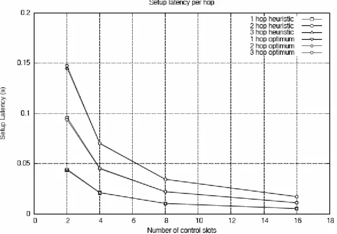
When the number of control slots decreases, however, the setup latency increases significantly. When the number of control slots increases from 2 to 16, which yields a decreasing MAC overhead from ~8% to ~66%. However, even though the minimum overhead is achieved, the setup latency is still in the order of hundreds of ms in all cases, which makes EBRP a suitable candidate for realistic applications, e.g. VoIP calls.
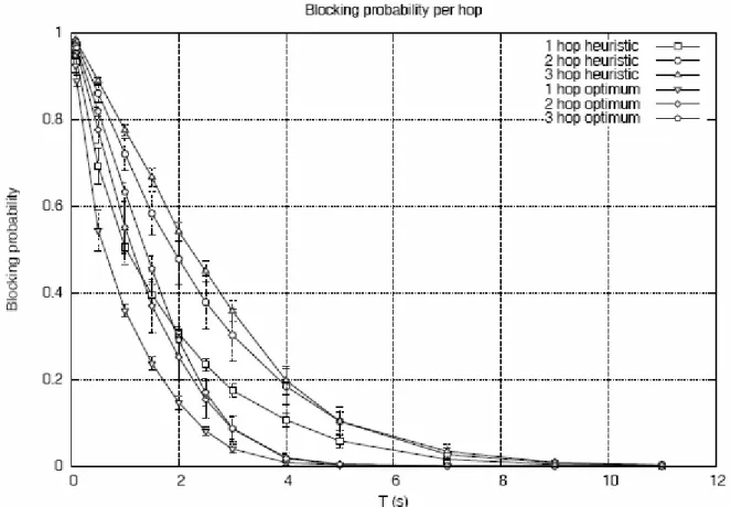
• Blocking probability: when the average interval between two consecutive calls at the same node (T) increases, as expected, the blocking probability decreases.
What is most interesting is that the blocking probability is not affected by the path length significantly. This is in contrast with the baseline scenarios of WMNs, where traffic flows that traverse more hops experience severely degraded performance with respect to traffic flows that have shorter path length (e.g. [13]).
Blocking probability is relatively small because the blocking probability BBi of any flow i can be
computed as: ( ) 1 1 i i e e B b ∈℘ = −
∑
− ,where be is the probability that there are not enough resources in link e so as to satisfy the
requirements of flow i, while ℘i is the set of links traversed by flow i. Therefore, BBi > BjB if
℘i ⊃ ℘j. However, in the evaluated scenario, be decreases with the distance from the receiver,
since links that are farther from the gateway tend to be less loaded due to spatial reuse, which is captured by the CAC procedure by means of the group partitioning.
12.1.1 First Scenario
• T = D.
• D = exponential with average 1, 2, 5, 10 seconds. • Number of control slots: 8.
• Bandwidth: 10 MHz. Setup latency
Setup latency is the same if we use heuristic or optimum algorithm and it proportionally increases with the number of hops.
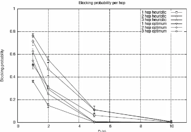
Blocking probability
Blocking probability is different with the optimum or heuristic algorithm, because if I use optimum algorithm the number of slots for each groups is bigger, since the number of groups is smaller.
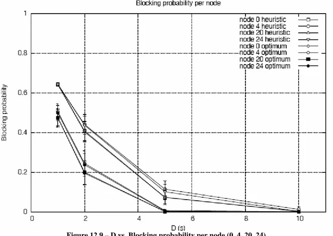
In the four vertices of the grid the blocking probability is the same because the load of the net is the same.
Figure 12.9 – D vs. Blocking probability per node (0, 4, 20, 24).
Number of flows
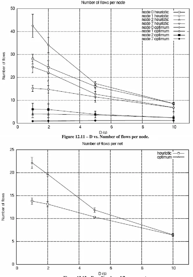
The number of flows increases near the gateways because in the gateways there is the maximum load, indeed, they are bottlenecks.
Figure 12.11 – D vs. Number of flows per node.
12.1.2 Second Scenario
• T = exponential with average 0.01, 0.05, 1, 1.5, 2, 2.5, 3, 4, 5, 6, 7, 9, 11 seconds. • D = exponential with average 2 seconds.
• Number of control slots: 8. • Bandwidth: 10 MHz. Setup latency
Setup latency is the same if we use heuristic or optimum algorithm and it proportionally increases with the number of hops.
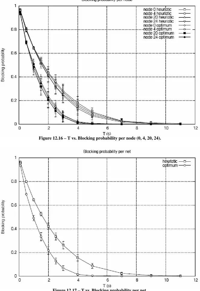
Blocking probability
Blocking probability is different with the optimum or heuristic algorithm because if I use optimum algorithm the number of slots for each groups is bigger, since the number of groups is smaller.
In the four vertices of the grid the blocking probability is the same because the load of the net is the same.
Figure 12.16 – T vs. Blocking probability per node (0, 4, 20, 24).
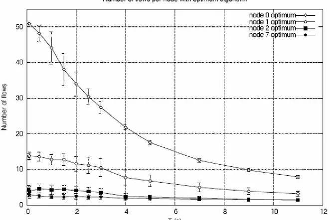
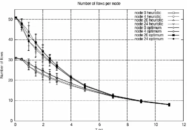
Number of flows
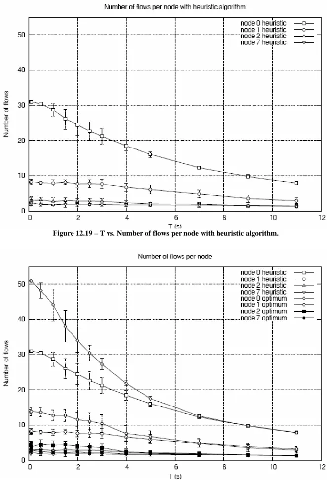
The number of flows increases near the gateways because in the gateways there is the maximum load, indeed, they are bottlenecks.
If we use optimum algorithm the number of admitted flows is greater.
Figure 12.19 – T vs. Number of flows per node with heuristic algorithm.
In the vertices the number of flows admitted is the most high possible.
12.1.3 Third Scenario
• T = 2 seconds. • D = 2 seconds.
• Number of control slots = 2, 4, 8, 16. • Bandwidth: 10 MHz
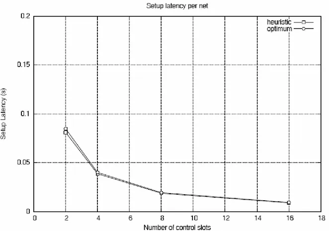
Setup latency
When the number of control slots decreases the setup latency increases significantly, which yields a decreasing MAC overhead, but the setup latency is still in the order of hundreds of ms in all cases.
Blocking probability
When the number of control slots increases the slots for data message decrease, so the blocking probability increases.
Figure 12.24 – Number of control slots vs. Blocking probability per hop.
12.1.4 Fourth Scenario
• T = exponential with average 4, 5, 7, 9, 11 seconds. • D = exponential with average 2 seconds.
• Number of control slots: 2. • Bandwidth: 5.5 MHz. In these configurations we have:
• 8 optimum groups Æ maximum 26 flows for each group. • 12 heuristic groups Æ maximum 17 flows for each group. Setup latency
In this configuration there are only two control slot, so the setup latency is worse that with the previous simulations.
Blocking probability
Blocking probability is different with the optimum or heuristic algorithm because if we use optimum algorithm the number of slots for each groups is bigger, since the number of groups is smaller.
In this configuration the number of slots for data message is bigger, so the blocking probability is smaller that with the previous simulations.
Number of flows
The number of flows increases near the gateways because in the gateways there is the maximum load.
Figure 12.30 – T vs. Number of flows per node with heuristic algorithm.
Figure 12.32 – T vs. Number of flows per node.
12.1.5 Fifth Scenario
• T = exponential with average 0.1, 0.5, 1, 1.5, 2, 2.5, 3, 4, 5, 7, 9, 11 seconds. • D = exponential with average 2 seconds.
• Number of control slots: 8. • Bandwidth: 10 MHz.
• 1 hop burst profile QAM 64 ⅔. • 2 hop burst profile QAM 16 ½. • Other burst profile QPSK ½. Setup latency
Setup latency is the same if we use heuristic or optimum algorithm and it proportionally increases with the number of hops.
Blocking probability
Blocking probability is different with the optimum or heuristic algorithm because if we use optimum algorithm the number of slots for each groups is bigger, since the number of groups is smaller.
It increases when increase the distance between source node and gateway but this increment is not meaningful because I use different burst profile.
Figure 12.37 – T vs. Blocking probability per node.
Number of flows
I use different burst profile, so I have the best number of admitted flows, because where the net is load I use QAM 64 ⅔ burst profile.
Figure 12.39 – T vs. Number of flows per node with heuristic algorithm.
Figure 12.41 – T vs. Number of flows per node.
12.2 Gateway
on
Center
Traffic flows are only established between an access point and the gateway. The center of the grid is the gateway, while the remaining nodes are access points.
Figure 12.43 – Gateway on center.
I assume all the access points to have the same workload, which consists of a set of G.711 VoIP calls [14].
Figure 12.44 – Flows with gateway on center.
I first assume that there are eight control slots per frame, which entails a moderate amount of MAC overhead due to transmission of control messages. In fact, about one third of the channel capacity is consumed by the control sub-frame.
In the totality of the simulations we notice that:
• Setup latency: if the control part of the MAC frame is over provisioned, the setup latency is only affected by the propagation delay of the PATH and RSV messages. This metric is greatly affected by the path length. Nonetheless, the absolute value of the setup latency is very small for all distances of the access points from the gateway, due to the forwarding of EBRP messages at the MAC layer.
• Blocking probability: when the average interval between two consecutive calls at the same node increases, as expected, the blocking probability decreases.
In this case, whereas the gateway is on the center, there is a bottleneck and the blocking probability is high.
12.2.1 First Scenario
• D = exponential with average 1, 2, 5, 10 seconds. • T = D.
• Number of control slots: 8. • Bandwidth: 10 MHz. Setup latency
Setup latency is the same if we use heuristic or optimum algorithm and it proportionally increases with the number of hops.
Blocking probability
Blocking probability is different with the optimum or heuristic algorithm because if we use the first the number of slots for each group is bigger, since the number of groups is smaller.
Figure 12.47 – D vs. Blocking probability per hop.
12.2.2 Second Scenario
• T = exponential with average 0.1D, 0.3D, 0.5D, 0.7D, D, 1.5D, 2D , 3.5D 5D, 7D, 8D, 10D seconds
• D = exponential with average 2 seconds. • Number of control slots: 8.
• Bandwidth: 10 MHz. Setup latency
Setup latency is the same if we use heuristic or optimum algorithm and it proportionally increases with the number of hops.
Blocking probability
Blocking probability is different with the optimum or heuristic algorithm because if we use the first, the number of slots for each group is bigger, since the number of groups is smaller.
Figure 12.51 – T vs. Blocking probability per hop.
12.2.3 Third Scenario
• T = exponential with average 2 seconds. • D = exponential with average 2 seconds. • Number of control slots: 2, 4, 8, 16. • Bandwidth: 10 MHz.
Setup latency
When the number of control slots decreases the setup latency increases significantly. When the number of control slots increases from 2 to 16, which yields a decreasing MAC overhead, but the setup latency is still in the order of hundreds of ms in all cases.
Blocking probability
When the number of control slots increases the slots for data message decrease so the blocking probability increases.
Figure 12.55 – Number of control slots vs. Blocking probability per hop.