CHAPTER
3
Characteristic Basis Function Method
Abstract- The objective of this chapter is to describe a new and efficient
strategy to solve linear systems encountered when method of moments is used for electromagnetic problems. This new approach permits the solution of electrically large problems by decomposing the traditional Method of Moments matrix into a certain number of blocks. It is based on the characteristic basic functions (CBFs). The CBFs are special basis functions defined on macro domains (blocks) that include a relatively large number of conventional sub-domains arising in a triangular or rectangular patch modeling of the objects. These new basis functions lead to a significant reduction in the number of unknowns. As a result, the size of the MoM matrix can be reduced to an order, which allows the use of a direct solver.
3.1 INTRODUCTION
Most methods for numerical calculation of electromagnetic fields are limited in their application to small objects, with respect to the wavelength, due to both the storage and execution time these methods require. The method of moments, which is based on integral equations, has the advantage of requiring unknowns only on the scattering body. However, to date, the application of MoM to large electromagnetic problems with linear dimensions of many wavelengths still poses considerable difficulties. The limitations are due to the resulting large and densely populated MoM matrix equations, which require huge amounts of memory and which lead to
prohibitively long computer running times when the resulting systems of equations are solved. The dimension of the moment matrix is equal to the number of employed basis functions, and in practice, an expansion in sub-sectional basis functions is preferred because of their flexibility for modeling arbitrary complex shapes. However, the functions must be defined densely enough to accurately approximate the unknown function and in order to guarantee a high accuracy of the results. This constraint, in turn, governs the rapid increase of the matrix size when large structures are studied. Recently, researches have investigated ways to circumvent the problems of high requirements of memory associated with storing of the Z matrix, and of computational time for solving the linear systems for large electromagnetic problems. A non-exhaustive list would include the impedance matrix localization (IML) [13], the sub-domain multilevel approach [14], the fast multipole method (FMM) [15 - 17], and the generalized sparse matrix reduction (GSMR), wavelet expansions basis to perform a sparse Z matrix. But, most of them are still bounded by a discretization size ranging from
λ
10 toλ
20, which makes the MoM matrix grow rapidly as the geometry becomes electrically large. When considering candidate moment-method discretization schemes, the ratio between the characteristic length scale of the scatterer and the wavelength plays a key role in determining the methodology of the solution. As long as the length scale is comparable to the wavelength, standard moment-method approaches are well suited. If the scatterer becomes large and contains a variety of length scales ranging from sub-wavelengths to several wavelengths, MoM becomes highly inefficient because of the rapid increase in the matrix dimension. In these cases, approaches based on blocks and macro basis concepts are better suited than the conventional MoM. In fact, they lead to smaller matrix size. The aim of the work developed in this chapter is the introduction of a technique for reducing the MoMmatrix to a relatively small and well-conditioned matrix that can be handled directly. This new approach, called the characteristic basis functions method (CBFM) [18], is based on the characteristic basis functions (CBFs),which are high level basis functions defined on larger domains, called blocks, than those used in the conventional Method of Moments. This, in turn, leads to a reduction in the number of unknowns. The CBFM is a general approach, since it can be applied to any arbitrary three-dimensional surface. It includes the mutual coupling effects rigorously and thus generates accurate solutions in a systematic manner.
3.2 CHARACTERISTIC BASIS FUNCTION METHOD
The conventional MoM formulation of the electromagnetic problem leads to a dense complex linear system of the form
Z J = (3.1) V
where Z is the generalized impedance matrix of dimension N× , J and V are N N× 1 vectors, and N is the number of unknowns. For large, complex problems, the matrix system (3.1) is used to solve for typically thousands of unknowns, which becomes difficult in terms of computer memory and computer running time, since they increase with Ο
( )
N2 and Ο( )
N3 , respectively. Conventional iterative solvers are more efficient than direct ones in solving equation (3.1) when N is very large, order on thousands, and one is interested in analyzing the problem for only a few excitation vectors V . It is often necessary to analyze RCS characteristic of a target for a wide range of incident angles, and it makes iterative solvers highly inefficient because they require solving again the linear systems (3.1) for each right hand side value. In such an analysis, the direct solvers are preferred because they give a matrix which is independent from the excitation, but are limited by the execution time. In this context, the idea to reduce or compress the number of unknowns for electrically large geometry by using high-level basis functions is a great advantage. In fact, it leads to a reduction in computational time and, if the final number of unknowns is small, a direct solver can be used. The proposed approach is oriented in this direction. The characteristic basis function method reduces the size of the matrix equation to a level so that the linear equation system can be solved directly without loss in accuracy of the solution, or deterioration of the condition number of the matrix. Also, it is independent of the type of basis/testing functions as well as of the integral equation used to formulate theproblem. The CBFM consists of separating the complex structure into various constituent parts, called blocks, characterizing these parts alone by using the so called
primary characteristic basis functions, which represent the self-interactions terms, and
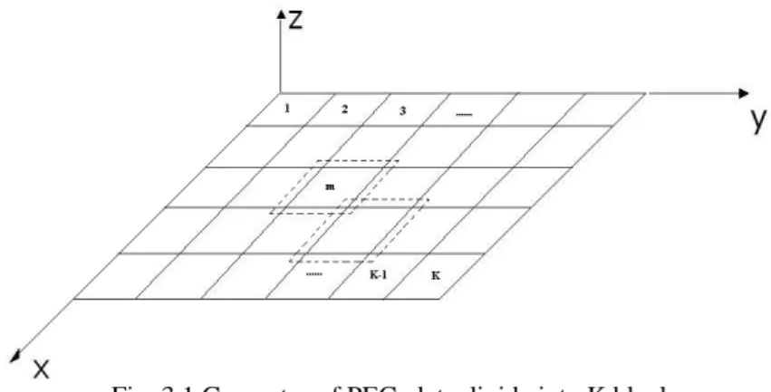
further “re-building” the complete structure properties using the characterization of these blocks and of their interactions with others blocks. These interactions are represented by the secondary characteristic basis functions, which describe the mutual coupling between individual blocks and the rest of the structure. The CBF method has three basic steps. First, the original geometry is divided into a number of blocks or macro-domains. Next, the primary and secondary CBFs are constructed for each block. Finally, the reduced matrix, the size of which is relatively small, is generated for the weight coefficients of the CBFs by using the Galerkin or other testing procedure, and it is solved directly. The reduced matrix generation can be considerably simplified by taking advantage of the symmetry of the block geometry. To illustrate the CBF method, we consider a PEC square plate. The first step is to partition the geometry into M
blocks with no real limitations on the dimension of the single blocks, as shown in fig. 3.1 in solid lines.
Fig. 3.1 Geometry of PEC plate divide into K blocks
Let N indicate the number of unknowns on the m mth domain, with m=1, 2,K,M . In order to obtain primary CBFs, all blocks are extended by a Δ gap in all directions. The
extended domains are shown in figure 3.1 in dotted lines. Now, we have M extended and partially overlapped domains and each of them has Nme unknowns, where
e
m m
N >N . The next step consists of extracting the Nme×Nme sub-matrix Zme, from the original N× MoM matrix N Z, for each of the M enlarged blocks. Then, this sub-matrix is used to determine the primary basis Jm( )m for the block m by solving the following linear sub-system
( )m ( )m ( )m
e m
Z J =V (3.2)
where V( )m is a subset of the original excitation vector V , and it is formed by extracting those Nme rows belonging to block m . The system 3.2 has to be solved M times for
each block, giving M primary basis functions, one for each domain. Even if the original number of unknowns N is large, because the geometry may be electrically large, the number of unknowns N in each extended block can be relatively small, so me
that equation (3.2) can be solved by an LU factorization. This type of decomposition is preferred since the (3.2) have to be solved several times in order to obtain secondary CBFs. In fact, this factorization has to be processed only one time and then the result can be stored, on hard disk or memory, and used whenever needed for generating the secondary basis of the relative domain. After the generation of primary basis functions, the secondary ones have to be calculated. These are obtained by solving equation (3.2) with different excitations. For each block, there are M −1 secondary basis functions which come from solving the equation
( )m ( )m ( )m
e k k
for k=1, 2,K,m−1,m+1,K,M and where m=1, 2,K,M . Jk( )m is the kth secondary basis for block m , and, Vk( )m is the excitation vector resulting from the mutual coupling
between block m and block k . It should be pointed out that there are two different situations for generating Vk( )m when equation (3.3) is solved. In the first situation, there are no common unknowns between the extended block m and block k . In this case, the excitation vector resulting from the mutual coupling between these two blocks is given by ( ) ( , ) ( ) , m m k k k k V = −Z J (3.4)
where Z(m k, ) is an Nme×Nk matrix formed from moment-method matrix Z by selecting the testing location at the extended block m , with the source located in the block k . In the second case, the enlarged block m shares some unknowns with the block k . Let
,
m k
N indicate the number of these shared unknowns. Now, it is important to avoid the common unknowns, which represent the part of the source in the observation block m , because we are interested in studying mutual coupling. In order to eliminate these source locations from Z(m k, ) and Jk( )k , we proceed to make them
(
,)
e
m k m k
N × N −N
matrix and
(
Nk−Nm k,)
×1 vector, respectively, by subtracting the Nm k, commonunknowns. After the excitation vector Vk( )m resulting from the mutual coupling has been found, the secondary CBFs can be computed for block k by solving equation (3.4) with matrix Ze( )m , which is already LU factored. This equation may be rewritten in
the following form
( ) ( ) ( , ) ( )
for , 1, 2, ,
m m m k k
e k k
where Z(m k, ) is a subset of the original MoM matrix Z and represents the interaction between macro-domains.
At the end of this procedure the number of characteristic basis functions is M , 2 M are primary bases and M M
(
− are secondary basis functions. Each domain has 1)
MCBFs, which are, then, elaborated to obtain an ortho-normalized basis function set by using the Gram-Schmidt procedure. In addition, this operation leads to an improvement in the condition number of the reduced matrix.
Now, the vector J of equation (3.1) can be expressed as a linear combination of the previous ortho-normalized CBFs ( ) ( )
[ ]
[ ]
( )[ ]
( )[ ]
( )[ ]
[ ]
( ) 1 2 1 2 1 2 1 0 0 0 0 0 0 k M M M k M k k k k k k M k J J J Jα
α
α
= = = ⎡ ⎤ ⎡⎡⎣ ⎤⎦⎤ ⎡ ⎤ ⎢ ⎥ ⎢ ⎥ ⎡ ⎤ ⎢ ⎥ ⎢ ⎥ ⎢ ⎥ ⎣ ⎦ ⎢ ⎥ = ⎢ ⎥+ ⎢ ⎥+ + ⎢ ⎥ ⎢ ⎥ ⎢ ⎥ ⎢ ⎥ ⎡ ⎤ ⎢ ⎥ ⎢ ⎥ ⎢⎣⎣ ⎦⎥⎦ ⎣ ⎦ ⎣ ⎦∑
∑
L∑
M M M (3.6)where,
α
k( )m , for m k, =1, 2,K,M , is the unknown complex expansion coefficient to be determined by using the reduced matrix, and, Jk( )m is the kth CBF of block m . The new expression of J is, then, substituted in equation (3.1), and, after carrying out the matrix-vector products, the result is an over-determined system of equations, which are cast in a matrix form as follows:( ) ( )1 1 ( ) ( )2 2 ( ) ( )
[ ]
1 1 1 1 , M M M M M k k k k k k N k k k Vα ϑ
α ϑ
α ϑ
× = = = + + + =∑
∑
L∑
(3.7) where ( ) 1, ( ) 2, ( ) , ( ) T i i i i k Z i Jk Z i Jk ZM i Jkϑ
= ⎣ ⎦⎡⎣⎡ ⎤⎣⎡ ⎤⎦ ⎣⎡ ⎤⎦⎡⎣ ⎤⎦ K ⎡⎣ ⎦⎤⎡⎣ ⎤⎦⎤⎦ .The next step in the proposed method is to generate a reduced matrix by applying the inner product to both the right and left sides of equation (3.6) with the use of Galerkin’s
procedure. The chosen testing functions are
ϑ
k( )i∗ for i q, =1, 2,K,M where ∗ is the adjoint. After performing the CBFM, the original system matrix Z has been reduced to a smaller one. This results in an 2 2M ×M linear system that is solved for the complex expansion coefficients α . Once the new unknowns α have been computed, the final solution J is calculated by substituting them in the expression (3.6). Reducing the
number of secondary CBFs can subsequently drop the size of the reduced matrix. This can be accomplished by performing a threshold procedure. For example, one way to realize the reduction of a secondary basis can be based on a distance criterion between the extended block m and the block k , but some a priori information about mutual
coupling levels is needed to utilize it. In fact, if the interaction is above a certain level it can be considered zero, and, consequently, we do not need to process the generation of the relative secondary bases.
At this point we are able to make some remarks on the proposed approach about execution time and RAM requirements. The most computationally intensive part of the CBFM is the LU factorization of the extended block matrix Ze( )m , which is used to compute the primary and secondary basis. Fortunately, this decomposition is independent of the excitation vector so it can be performed only once and stored. The computer running time is proportional to Nme3 for each Ze( )m matrix where Nme is the size of the extended block m . The rest of the process in the CBFM involves only matrix vector products and ortho-normalizations. Also, the Characteristic Basis Functions Method realizes a reduction in the storage requirement, which is proportional
only to
{ }
1,2 , , 2 max m M e Nm = ⎡ ⎤⎣ K ⎦ and not to N , which is the number of unknowns in the original problem 3.1. Not only does CBFM lead to a saving in memory and time but it also can handle very large problems that are unsolvable using conventional techniques, and it is
very suitable for parallel processing. On the other hand, the CBFs, obtained by solving equations (3.3) and (3.4), are dependent on the frequency and excitation. In the next section, a new and faster method for calculating CBFs, which leads to excitation independent basis functions, is introduced. It is based on the plane wave spectrum and singular value decomposition (SVD).
3.3 IMPROVEMENT OF THE CBFM
The CBFM can be improved, in the sense of reducing computational effort, by avoiding secondary characteristic basis function evaluations that require several matrix-vector products. Giving more degrees of freedom to primary CBFs can eliminate secondary ones. In order to accomplish this, we can use a spectrum of plane waves, as source, instead of the single incident wave, which was used in the previous section, to compute the primary basis. In this way, multiple incident angles are covered. It is necessary to point out that now each block will have more than one primary CBF. This new procedure requires SVD to reduce the number of CBFs for each block, as, will be illustrated.
3.3.1 Singular Value Decompositon
The SVD is the single most important matrix decomposition for numerical methods and theory. It decomposes a matrix into the product of three matrices: two orthogonal matrices and one diagonal matrix. Consider an n×p matrix X . The SVD of matrix X leads to the following factorization
t
where U is an n×p orthogonal matrix, V is ap×p orthogonal matrix and, D is a
k k× diagonal matrix of the form
1 2 0 0 0 0 0 0 k
σ
σ
σ
⎡ ⎤ ⎢ ⎥ ⎢ ⎥ ⎢ ⎥ ⎢ ⎥ ⎢ ⎥ ⎢ ⎥ ⎣ ⎦ L L O M M O O O M M O O L L (3.9) where k=min( , )n p .The diagonal entries of D can be required to be ordered as
σ
1≥σ
2 ≥L≥σ
k ≥0.These diagonal elements are the singular values of X and they are usually stored from largest to smallest. Singular values of zero or near zero indicate that the matrix is singular or ill-conditioned.
Some properties of the SVD:
1) If r=rank X( ), then
σ
r+1=K=σ
k =0. 2) 1 2 Xσ
= 3) 12 2p 2 F Xσ
+ +Kσ
=4) The minimum norm least squares solution to Xa= is given by b a* =VD U b† T , where D is the † p×p diagonal matrix with diagonal entries
1 † if 0 0 if 0 i i i i
σ
σ
σ
σ
− ⎧ > ⎪ = ⎨ = ⎪⎩ (3.10)3.3.2 Plane Wave Spectrum and CBFM
In this subsection, a variant of CBFM that does not require computing secondary CBFs is introduced.
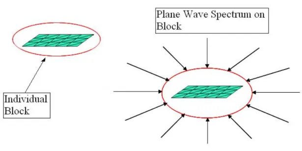
To avoid the computational of secondary CBFs, we proceed to use a plane wave spectrum, as figure 3.2 shows. The original RCS problem, represented by equation (3.1), has been formulated by specifying only one plane wave excitation. However, in this case it is still contemplated in the new approach because one of the PWS excitations would be the original one.
Fig. 3.2 PWS on a block
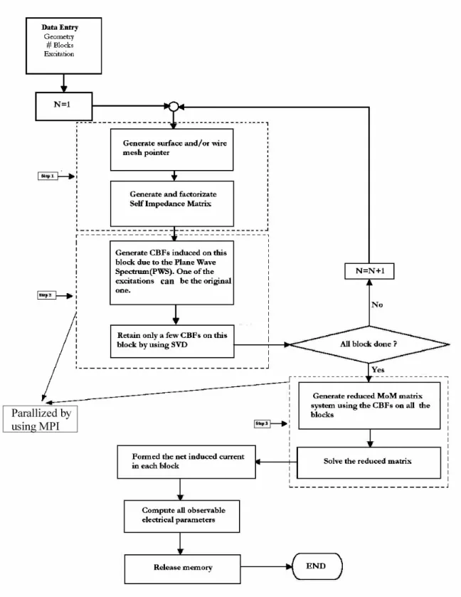
We start by considering an arbitrarily shaped geometry and analyzing it by using the conventional Method of Moments that leads to the equation (3.1). Let N be the number of unknowns obtained by applying the MoM, so that the impedance matrix Z
is an N× matrix. The new CBF approach is presented with the help of the flowchart N
Fig. 3.3 Flowchart outlining the various steps in the CBFM
The first step consists of portioning the original target. The geometry, and consequently the matrix Z, is divided into a number of blocks, for example K. These blocks can have different sizes, but we assume they have the same dimension N . In order to b
compute the CBFs, all blocks are extended by a Δ in all directions. Each of the K
extended blocks is represented by the relative Nbe×Nbe self-impedance matrix Z , ii
where i=1, 2,K,K and Nbe is the number of unknowns in the extended blocks. This matrix is generated by extracting it from the original MoM matrix, and it is then used to generate the CBFs induced on the relative block by exciting the block with a windowing plane wave spectrum. The excitation is obtained by taking several incoming plane waves with different incident angles
(
ϑ φ
,)
. Let Nϑ and Nφ indicate the numberof samples for ϑ and
φ
, respectively. This results in a total of N Nϑ φ wave planes and the same number of primary CBFs on each block, which are determined by solving the following linear system, m PWS ii i i Z J =V (3.11) where Jim is the th
m CBF’ Nbe×1 vector of the block i (i=1, 2,K,K), and 1, 2, ,
m= K N Nφ ϑ, andViPWS is the excitation’s vector of the relative CBF. The system
(3.11) has to be solved N Nϑ φ times for each block to obtain the complete set of CBFs.
After computing all the primary bases of block i, we can order them in a matrix that is indicated as J . This is an ii
e b
N ×N Nϑ φ matrix. In order to reduce the number of CBFs,
the previously introduced CBFs’ matrix is factored by using SVD decomposition. The
ii
J is expressed as the product of three matrices
t
=UDV , 1, 2, , ,
ii
J i= K K (3.12)
where U is an Nbe×N Nϑ φ orthogonal matrix, V is an N Nϑ φ×Nbe orthogonal matrix, and D is an N Nϑ φ×N Nϑ φ diagonal. As explained in the previous subsection, the
elements of the latter matrix are the singular values of Z . At this point a thresholding ii
procedure is used on the singular values to reduce the number of CBFs. This procedure works by defining a ratio between singular values as follows:
max , j 1, 2, , . j j R σ N Nφ ϑ σ = = K (3.13)
The above quantity is then compared with an appropriated threshold. If it is over a well-chosen level, the correspondent singular value is posed to zero. Suppose this happens for j=M+1 with M <N Nϑ φ, the number of retained primary bases is equal to M . In this way, we have reduced the primary characteristic basic functions from N Nϑ φ to M
for the blocks i. It is important to observe that, for a scatterer compactly supported within a sphere of radius a there is a sharp cut-off after which the asymptotic behaviour of the singular values takes hold.
-0.2 0 0.2 0.4 0.6 0.8 1 0 100 200 300 400 500 600 700 8 00 Block 15 Block 1 Block 2 Block 23 No rm al iz ed Sin g u lar V a lue s Index
Fig. 3.4 Distributions of the normalized singular values for some blocks
Figure 3.4 shows the distribution of the normalized singular values for the corner reflector case, which is presented in the numerical section. Distributions of the singular
values, plotted for different blocks, show a sharp transition region where the cut-off occurs. This cut off can be estimated analytically. For the sake of simplicity, we assume that all of the blocks contain the same number M of CBFs. Hence, if the original geometry is divided into K macro-domains, this gives a total number of KM CBFs. The original unknown J can still be expressed as a linear combination of the new basis functions in a similar fashion to equation (3.6) where αk are the unknowns to be
determined. The final step is to generate the reduced KM×KM MoM matrix for the
KM unknown complex coefficients αk by performing the inner product on equation
(3.1) after substituting the new expression of J in it. The form of reduced MoM matrix is as follows
[ ]
† † † 11 11 11 11 12 22 11 1 † † † 22 21 11 22 22 22 22 1 † † † 1 11 11 22 K KK K KK KM KM KK K KK KK KK KK J Z J J Z J J Z J J Z J J Z J J Z J Z J Z J J Z J J Z J × ⎡ ⎤ ⎢ ⎥ ⎢ ⎥ = ⎢ ⎥ ⎢ ⎥ ⎢ ⎥ ⎢ ⎥ ⎣ ⎦ L L M M O M L (3.14)where Zmn is the coupling matrix linking block m and n , J is the CBF matrix of ii
block i. Note that each of the inner product entries in the above equation results in a matrix of size M×M, and the MoM matrix reduction involves M complex matrix-vector products. It is possible to reduce this number by invoking reciprocity of source and fields blocks. Inner products in equation 3.14 are taken with respect to the adjoint of CBFs on field blocks in order to obtain least mean square (LMS) error. As a result
† †
mm mn nn nn nm mm
J Z J ≠ J Z J (3.15)
even if the individual Zmn matrices are symmetrical. However, it is still possible to simultaneously generate the reduced sub-matrices linking
(
n m and ,)
(
m n blocks by ,)
converting the complex-matrix vector operations into real operations. By using thisstrategy, the complexity in the generation of (3.14) matrix is reduced from M to 2
M .
We are in the position to make some statements about the memory and execution time the new CBF method requires. The most computationally intensive parts are the generation of the self-matrix of each block, and the generation of the reduced matrix, both of parts are indicated in the flowchart of figure 3.3 as the second and third step. Fortunately, these two tasks can be parallelized by using the MPI library. Also, there is an additional overhead due to the factorization of each individual block. Since the CBFs are independent of incident angle, this factorization is done one time, and the same CBFs can be reused for multiple incident angle directions in a scattering problem. This means that the reduced matrix is independent of the excitation. As a result, it is trivial to solve a problem for multiple excitations. Moreover, if the geometry inside a particular block is altered, only the CBFs that belong to it need to be recomputed. As the preceding CBF version, this new approach of CBFM keeps a reduced primary memory requirement, which is only proportional to the square of the block’s self-matrix size.
3.4 CONCLUSION
In this chapter, an efficient approach has been presented to solve a large and dense system of linear equations arising in the integral-equation formulation of an electromagnetic problem. Unlike the many existing methods to sparsify large moment problems, we have proposed an approach to split the moment analysis into several smaller sub-problems. The procedure is based on a geometric division of the problem into so called blocks. We have successfully illustrated its effectiveness and accuracy with several examples. In fact, each case has shown a generally good agreement, making the CBFM a elegant and powerful method to solve the MoM matrix system. In
addition, a reduction in time and memory required has been ascertained, and mainly we have demonstrated that it is possible to solve electrically very large problems.