Micro-scale dispersion modelling with background correction to simulate air quality in Milan

MICRO-SCALE DISPERSION MODELLING

WITH BACKGROUND CORRECTION TO

SIMULATE AIR QUALITY IN MILAN

A. PIERSANTI, L. VITALI

Dipartimento Sostenibilità deiSistemiProduttivie Territoriali Divisione Modellie tecnologie per la riduzione

degliimpattiantropicie deirischinaturali Laboratorio Inquinamento Atmosferico

Cent

Centro Ricerche Bologna

RT/2017/6/ENEA

ITALIAN NATIONAL AGENCY FOR NEW TECHNOLOGIES, ENERGY AND SUSTAINABLE ECONOMIC DEVELOPMENT

F. RUSSO, M. ADANI, L. CIANCARELLA A. PIERSANTI, L. VITALI Dipartimento Sostenibilità dei Sistemi Produttivi e Territoriali Divisione Modelli e tecnologie per la riduzione degli impatti antropici e dei rischi naturali Laboratorio Inquinamento Atmosferico Centro Ricerche Bologna

MICRO-SCALE DISPERSION MODELLING

WITH BACKGROUND CORRECTION TO

SIMULATE AIR QUALITY IN MILAN

RT/2017/6/ENEA

ITALIAN NATIONAL AGENCY FOR NEW TECHNOLOGIES, ENERGY AND SUSTAINABLE ECONOMIC DEVELOPMENT

I rapporti tecnici sono scaricabili in formato pdf dal sito web ENEA alla pagina http://www.enea.it/it/produzione-scientifica/rapporti-tecnici

I contenuti tecnico-scientifici dei rapporti tecnici dell’ENEA rispecchiano l’opinione degli autori e non necessariamente quella dell’Agenzia

The technical and scientific contents of these reports express the opinion of the authors but not necessarily the opinion of ENEA.

MICRO-SCALE DISPERSION MODELLING WITH BACKGROUND CORRECTION TO SIMULATE AIR QUALITY IN MILAN

F. Russo, M. Adani, L. Ciancarella, A. Piersanti, L. Vitali

Abstract

Urban air quality is raising great interest in recent years, for studying both the impact of pollution on human health and the causes of periodic pollution exceedances in urban areas. This is a “high resolu-tion” problem that has to be treated with high resolution dispersion models. Unfortunately with the present day computational facilities, these models cannot take into account large areas (more than few kilometers) or long periods (more than few days) and the real complexity of atmospheric chemical reactions due to their Lagrangian approach. Here we studied the feasibility of introducing the model Micro-Swift-Spray (MSS) in the AMS-MINNI air quality chain, setting up an experiment to study the suitability of the regional component of AMS-MINNI (FARM) as a background provider for MSS. The results of this experiment indicate that on a daily average the background correction provided by FARM greatly improves the performance of MSS compared to traffic air quality station measurements. On the other hand the hourly performance of this correction is not as encouraging, but it is probably due to some common assumptions made in the preparation of the emission data that feed the MSS. Key words: urban air quality, micro-scale modeling, background concentrations, validation.

Riassunto

La qualità dell'aria in ambiente urbano sta sollevando grande interesse negli ultimi anni, per lo studio sia dell'impatto dell'inquinamento sulla salute umana che delle le cause dei superamenti periodici dei limiti di legge nelle zone urbane. Questo è un problema ad alta risoluzione che deve quindi essere af-frontato con modelli di dispersione ad alta risoluzione. Purtroppo con gli strumenti di calcolo di cui di-sponiamo oggi, questi modelli non possono tener conto di aree molto estese (non più di pochi chilometri) o di lunghi periodi di tempo (non più di pochi giorni) e della reale complessità delle reazioni chimiche in atmosfera a causa del loro approccio lagrangiano. In questo studio abbiamo esaminato la possibilità di introdurre il modello Micro-Swift-Spray (MSS) nella catena modellistica AMS-MINNI, rea-lizzando un esperimento per studiare l'idoneità del modello di dispersione chimica regionale di AMS-MINNI (FARM) come fornitore delle concentrazioni di fondo necessarie ad MSS. I risultati di questo esperimento indicano che su una media giornaliera la correzione del fondo fornita da FARM migliora notevolmente le prestazioni del MSS rispetto alle misure di una stazione di traffico. Nonostante questo le prestazioni orarie di tale correzione non sono altrettanto incoraggianti, e la causa è probabilmente da ricercare nelle ipotesi comunemente fatte in sede di preparazione dei dati di emissione che alimen-tano il modello MSS.

Parole chiave: qualità dell’aria in ambiente urbano, modelli a micro-scala, concentrazioni di fondo, validazione.

1. INTRODUCTION

2. THE MODELLING SUITE: MICRO-SWIFT-SPRAY AND AMS-MINNI 2.1 Micro-Swift

2.2 Micro-Spray

2.3 Background contribution: AMS-MINNI 3. THE EXPERIMENT

4. RESULTS AND DISCUSSION 5. CONCLUSIONS 6. REFERENCES 7 9 9 9 10 11 17 20 25

INDEX

7

1 INTRODUCTION

Air quality in urban areas is a high resolution problem that has to be treated with a high resolution model. The density of population and polluting activities, the complexity of the urban topography influencing local meteorological regimes, the temporal variability of emissions are a challenging mix for a reliable model description. This is unavoidable for health impact assessments in urban areas, as the variability of concentrations strongly influences the actual personal exposure to pollutants.

Aside traditional and simple model approaches like regression models of measured concentrations (e.g. De Hoogh et al., 2014) and Gaussian models (e.g. Lefebvre et al., 2011), in the last years the interest is growing towards models with more complex physical description that can reach very high resolutions to allow studying in detail the transport and impact of traffic pollution on a few meters scale, relying on growing availability of affordable computing power. In the following, such models are called “micro-scale models” (MSMs). Unfortunately, MSMs still suffer from the usual trade-off between spatio-temporal detail and generality, as they cannot take into account large areas (more than few kilometres) or long periods (more than few days) due to their computational demand and the real complexity of atmospheric chemical reactions due to their Lagrangian nature that makes chemical reactions difficult to be parametrized. Constrained focusing on small areas requires on one hand to take into account external contributions to concentrations in the focus area, which can be substantially depending on the local situation. On the other hand, MSMs typically do not have the capability to compute the chemical transformations of pollutants together with the transport, and in the case of urban air quality, where local emissions, mainly from road traffic and domestic heating, are typically very reactive (like nitrogen monoxide – NO and organic compounds – VOCs), chemical transformations cannot be neglected.

In order to take into account both these issues, some modellers are introducing chemical transformations in their MSMs, increasing the demand for computing efficiency (Kaplan et al., 2014). An alternative approach is to provide the background contribution, including primary and secondary pollutants transported from outside the urban area, to be added to the high resolution simulations (Arunachalam et al., 2014).

ENEA carried out MSMs simulations on several Italian cities, in the framework of a 2011-2015 collaboration agreement signed with the Italian Ministry of the Environment, aimed to start a new national network of special purpose air quality stations. In order to reach the proper spatial detail to assess the representativeness of “urban traffic” air quality stations, placed in the built urban environment and influenced mainly by road traffic emissions, we used a urban micro-scale model (Micro-Swift-Spray, MSS). We then studied the feasibility of introducing MSS in the AMS-MINNI (Ciancarella et al., 2016) air quality chain, providing complete coverage of model concentrations on Italy. We set up an experiment to study the suitability of the regional component of AMS-MINNI as a background provider for MSS.

8

This report presents the main findings of the experiment. It is divided into four main sections. Section 2 describes the modelling suite, presenting each part of the MSS model and the FARM model which will provide the background simulation. Section 3 describes in detail the setup of the experiment and section 4 sums up the results and presents some points of discussion.

9

2 THE MODELLING SUITE: MICRO-SWIFT-SPRAY AND AMS-MINNI

The Lagrangian model SPRAY was developed in Italy by Arianet Ltd. and applied, over the last 25 years, in many studies. SPRAY is suitable for describing industrial pollution, with domains of the order of tens of km and resolutions of the order of hundreds of meters, as well as urban pollution, with domains of the order of hundreds of meters and resolution of the order of meters. To take into account a specific urban orography, the model has a dedicated version called Micro-Swift-SPRAY (MSS; Tinarelli et al., 2007), described in the following section. MSS has already been applied for simulating dispersion in street canyons, in Paris (Duchenne et al., 2011), Bologna (Poluzzi et al., 2006), Torino (Tinarelli et al., 2009) and Milano (Tinarelli et al., 2013).

The MSS system is dedicated to the simulation of dispersion on urban terrain, with the presence of obstacles to the movement of the vertical wind: this is a key feature to reproduce atmospheric flows inside the canyon roads, i.e. the volumes bounded by roads and adjacent buildings, inside of which traffic measuring stations are almost always placed. The module responsible for the reconstruction of the wind field in the presence of obstacles is called Micro-Swift. Once the turbulent wind field is obtained, the dispersion of pollutants using a Lagrangian dispersion code (Micro-Spray) is calculated, wherein the mass particles bounce off the ground and on the obstacles and the time resolution can be adjusted to follow the strong weather field gradients. Compared to more complex models, for example the CFD (Computational Fluid Dynamic), the Lagrangian approach and meteorology diagnostics allow for a significant saving of computing resources, making the tool suitable for feedback of multiple sources with time intervals of the order of a year (Moussafir et al., 2010).

2.1 Mi cro- Sw if t

Swift is a mass conserving interpolator over complex terrain (Tinarelli et al., 2007) which is used for the preparation of the necessary meteorology for the model Spray. Micro-Swift is the version of Swift adapted to the urban scale, with a description of the obstacles represented by the buildings. This description is made operationally by the module SHAFT (Shape to SWIFT), which defines the vertical obstacles from shapefiles buildings description in terms of polygons, with the attribute height above the ground. Given a topography, a low resolution meteorology and the description of the buildings as vertical obstacles, the high resolution 3D Micro-Swift wind field is generated as follows. The first hypothesis of the field is calculated by interpolation. This first hypothesis is modified empirically taking into account the obstacles. The flow is corrected to satisfy the continuity equation and considering the permeability of the soil and of the obstacles. Micro-Swift also comes with turbulence diagnostics (i.e. a field of turbulent kinetic energy TKE) which will then be considered by Micro-Spray for the dispersion. The TKE is calculated taking into account the balance between production and dissipation terms.

2.2 Mi cro- Spray

Micro-Spray is a Lagrangian particle dispersion model derived directly from Spray, which takes into account the presence of vertical obstacles. The dispersion of pollutants is simulated by considering the motion of a

10

large amount of particles each with a fraction of the mass emitted by the source. The motion of the particles follows an equation in which the speed is divided into two components, an average speed defined by local wind reconstructed by Micros-Swift and a stochastic component which simulates the atmospheric turbulence. The stochastic component is obtained from the solution of the three-dimensional Langevin equation for random speed. The Lagrangian time scales and the variance of the wind speed are derived from the TKE and the rate of dissipation is calculated by Micro-Swift.

2.3 B ackground cont ri bu ti on: AMS - MIN NI

The MINNI (National Integrated Model to support the international negotiation on atmospheric pollution) model is an ENEA project, born in 2002 and funded by MATTM (the Italian Ministry for Environment and Territory and Sea), to develop a tool able to link policy and atmospheric science, and to assess the costs of the abatement measures. MINNI is composed by two main elements: the national AMS (Atmospheric Modelling System); and the national Integrated Assessment Model GAINS-Italy (Greenhouse Gas and Air Pollution Interactions and Synergies Model over Italy). The AMS is a multi-pollutant Eulerian Atmospheric Modelling System simulating meteorological fields and computing gas and aerosol advection, diffusion and chemical reactions in atmosphere (Mircea et al., 2014), based on the model FARM (Flexible Air Quality Regional Model, Silibello et al., 1998, 2008; Gariazzo et al., 2007; Kukkonen et al., 2012) a three-dimensional Eulerian model that includes transport and multiphase chemistry of pollutants in the atmosphere.

Various agreements finalized between ENEA and MATTM between 2002 and 2008 have led over the years to various developments and applications of modelling system MINNI. Since 2010, in fulfilment of Legislative Decree no. 155/2010 (Art. 22, paragraph 5), ENEA is required to draw up every five years, and for the first time in the year 2010, modelling simulations of air quality on a national basis and to make the results of such calculations available to the Regions and autonomous Provinces for their air quality assessments. The 2010 results are available in a dedicated ENEA technical report (Ciancarella et al., 2016).

11

3 THE EXPERIMENT

The analysis is focused on NOx concentrations, as in urban areas they are strongly determined by local sources, mainly road traffic and domestic heating, therefore a detailed description of microscale dispersion phenomena near the emission sources is required.

The Milan urban environment was chosen for this experiment. In particular, the modelling simulation is focused on the description of pollutant concentrations patterns in the surroundings of Milano Senato air quality station, whose monitoring data are used for the validation of the modelling results . This site is located 1 km away from the city centre, on the inner ring road, and is classified as traffic urban, according to the EOI classification scheme (European Council, 1997).

MSS can be used, at the resolution of meters, with reasonable computing times, on a dominion of few kilometres. Recently it has been upgraded to simulate concentrations in an entire city with that fine resolution, but with necessary HPC support and code parallelization (Kaplan et al., 2014). Since MSS does not use initial or boundary conditions, it will not be able to simulate the contributions due to the transport from parts of the city that are outside of its calculation domain. The successful use of FARM as a background provider for MSS simulations requires to be able to set up a FARM simulation which takes into account all the contributions to concentrations that cannot be simulated by MSS: local emissions not included in MSS, secondary NOx that is produced by photochemical processes, NOx transported in from outside the MSS domain.

The improved version of the MSS simulation consists in adding to it the NOx concentrations calculated with FARM by zeroing out the emissions in the MSS domain (Arunachalam et al., 2014), as these emissions are included in the MSS model run. Therefore the corrected MSS concentrations in every simulation cell will be:

MSSc (s,t) = MSS (s,t) + FARMb (t) (1)

where MSSc is the MSS concentration corrected with the FARM background, MSS is the regular MSS concentration and FARMb is a background simulation obtained by zeroing out the emissions in the MSS domain. The variables s and t indicate space (within the MSS domain) and time.

The model grids of MSS and FARM have to be coherent, with MSS domain covering exactly one or more FARM grid cell. This is the key assumption to avoid double counting of emissions, as FARM zeroed emissions are exactly transferred into the microscale model.

Assuming there is only one FARM cell over the MSS domain, the FARM background here is considered space independent, thus only time dependent. Therefore the corrected MSS data will have a time modulation that depends both on the MSS modulation and the FARM modulation. If we want to keep only the MSS modulation in the corrected data, we will have to use the equation:

12

where FARMb is the time interval average of FARMb (t). This allows to mitigate the influence of FARM time patterns, coherent with the detail of a national-scale model with top-down emissions, on MSS time patterns, in principle deriving from local emission data with higher detail.

It should be emphasized that in general MSMs require emission data and orography of consistent spatial detail. In urban areas, the starting point is information on emissions from vehicular traffic flows on the road network, along with the three-dimensional urban topography, especially buildings. Major contributions to concentrations usually come from residential heating, but detailed data and inventories are more difficult to find.

3.1 MSS m i croscal e si mu l ati on

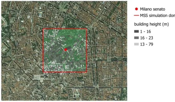
In this study, road traffic emission data were made available by the Environmental and Transport Agency (AMAT) of the Municipality of Milano. The data of three-dimensional urban topography were extracted from the National Cartographic Portal of the Ministry of the Environment, via QGIS procedures. The simulations were carried out at a resolution of 2 m. The meteorological year used is 2010, to allow the use as input fields of the prognostic meteorological model at a resolution of 1 km, already available from the Special Purpose Stations activities. The domain on which the simulations were conducted was centred on the station of interest, with size 1 km x 1 km (500x500 points), and is shown in Figure 1. Being the MSS domain a small part of the central urban area of Milan, the contribution of the urban pollution transported from outside the MSS domain will not be negligible.

Figure 1: Milano Senato air quality station (red dot with geographic coordinates: 45.4695 N, 9.1980 E) and the MSS simulation

domain.

Gridded emissions were provided in terms of grams per year (2010) and in UTM32 coordinates. For use in MSS, transformation of the cell emissions into linear emissions was required, made in ArcGIS assigning

13

each emitting cell to the nearest road section. The temporal modulation was performed following the modulation profile in Figure 2.

Figure 2: Time modulations of the MSS emissions, in terms of hourly percentage of the total daily value.

The specie of interest for this simulation is NOx, whose emissions spatial distribution within the domain is shown in Figure 3.

Figure 3: NOx emissions for the selected domain around the station of Milano Senato. The value for the road segment

close to the monitoring station is approximately 657 kg / year. 0.0% 1.0% 2.0% 3.0% 4.0% 5.0% 6.0% 7.0% 8.0% 1 3 5 7 9 11 13 15 17 19 21 23

Emission time modulation

14

The concentrations of pollutants near traffic pollution monitoring stations typically have a high spatial variability (Zauli Sajani et al., 2004; Vardoulakis et al., 2011). Also the limit values for the various pollutants are usually fixed over long periods of time, and then to perform a study of representativeness is necessary to run simulations on the same time scale. MSS presents various difficulties to be used for very long simulations, not least the computational effort and the storage of the results. For these reasons, we choose to simulate shorter periods (days) and we choose a set of days in which the wind was representative of the directions and intensity of winds prevailing in the areas of interest during the year. Running MSMs only on a set of inlet wind directions and using a numerical combination of these to compute the final results is commonly used in the literature (eg. Santiago et al., 2013). The choice of the most representative days was based on the frequency of winds produced at 1 km resolution, in function of both direction and intensity. The chosen days for the representativeness study are listed in table 1. Amongst these daily model runs, we chose the ones that had a complete 24 hour record of station measurements and these are highlighted in red in table 1.

In Figure 4 we can see an example of the NOx concentration field calculated with MSS, on May 10 2010 at 18:00. NOx accumulations along the main roads are clearly visible.

Milano Senato

Date Wind direction Wind intensity (m/s) Yearly frequency

22-01-2010 N 1.0-2.0 0.26 03-02-2010 N 2.0-3.0 0.12 10-05-2010 E 2.0-3.0 0.18 02-09-2010 NE 1.0-2.0 0.08 08-09-2010 E 1.0-2.0 0.06 08-10-2010 NE 2.0-3.0 0.09 20-10-2010 NO 2.0-3.0 0.15 11-12-1010 NO 1.0-2.0 0.06

Table 1: daily average wind direction and intensity for the days chosen for the representativeness study. The cases in red are

15 Figure 4: NOx concentration simulated by MSS for the day 10 May 2010 at 18:00.

3.2 F ARM bac k groun d si mul ati ons

As already stated in section 3, due to the lack of a chemistry module, the MSS NOx simulation does not take into account any secondary component. Moreover, when used on a domain which is included in a larger urban area (as in this case), the MSS NOx simulation cannot take into account any mass of pollutants being transported from outside the domain. Therefore we expect the MSS concentration fields to be systematically lower than those measured by air quality stations thus requiring a way to add the missing part. In our particular case we had a regional dispersion model, FARM, that includes a complete chemistry model and a complete and tested setup on the MSS simulation area. We wanted to test how this model behaves as a background provider for MSS.

In order to do so, we set up a simulation with FARM on a domain such that one FARM cell would cover exactly the MSS domain, granting in this way that we could have a direct comparison between the FARM and the MSS emissions in the FARM cell – MSS domain. A partial overlap between MSS domain and the FARM grid cell would result in different spatial reference of MSS and FARM emissions, preventing the use of the FARM emissions zeroing approach. Figure 5 helps clarifying this setup showing a portion of the FARM simulation overlapped with the entire MSS simulation, both corresponding to the NOx concentrations simulated on May 10 2010 at 18:00.

16

Figure 5: NOx concentrations obtained with FARM at the resolution of 1km x1km and the MSS NOx concentrations on the

MSS domain, which fits in a single FARM pixel.

The second aspect that needed to be considered for this coupling was how the emissions related between the two simulations. FARM emissions derive from the top-down Italian emission inventory at NUTS3 (province) level, with road traffic data from national statistics of vehicle mileage and spatial disaggregation with proxy variables, that for urban road traffic is the population density. MSS emissions were provided by AMAT, calculated with the same methodology (EEA, 2013) of the national inventory, but with different road traffic data (local counting and assignment model) and bottom-up approach. Upon careful computation it turned out that the total NOx yearly emissions used in the MSS simulation were 2.45 times smaller than the total NOx yearly emission used by FARM in the same cell. Since the modulation profiles used to compute the hourly emissions in the two cases are very similar, in order to compare the NOx concentrations simulated by MSS with those simulated by FARM, the first ones will have to be corrected for this factor.

17

4 RESULTS AND DISCUSSION

Here the results of the three days simulations are shown. The daily average comparisons are shown in Figure 6 and 7, in terms of simple average concentrations and percentage differences respectively.

Figure 6: NOx daily concentrations on the 3 analysed days: the red bars show the air quality station data, while

the blue bars show the MSS simulation data. The light green bars show the daily means obtained with FARMb and the other two colour bars represent two different corrections to MSS using FARM background simulation (violet: MSS corrected by equation (2); light blue: MSS corrected by 2.45).

Figure 7: Percentage difference between the measured daily means of NOx and those obtained respectively

0 20 40 60 80 100 120 140 160 180 200 20100122 20100510 20100902

daily mean Milano_senato MSS

Daily mean FARM MSSc 2.45*MSS+FARMb m icro g/ m 3 0 10 20 30 40 50 60 70 80 90 100 20100122 20100510 20100902 MSS

Daily mean FARM MSSc

2.45*MSS+FARMb

18

by MSS (blue), FARMb (light green), MSSc (violet) and the full MSS correction (light blue).

For all cases, MSS strongly underestimates measured concentrations. The FARM background correction to MSS clearly reduces discrepancies with measurements, with good performance both on January 22th, winter day with a high average, and on May 10th, late spring with low concentration. On September 2nd, MSS with no emission correction behaves better than MSS with 2.45 emission correction. Therefore we can say that MSS on a daily average agrees significantly better with the measurements if corrected for the background obtained by FARM, with a satisfactory reproduction on daily averages.

Figure 8 shows the same results on hourly basis.

Figure 8: NOx hourly concentrations simulated by MSS (purple), measured by the Milano Senato station (blue), FARMb

(green) and the finally corrected MSS (red), for the case studies January 22 2010 (a), May 10 2010 (b) and September 2 2010 (c).

19

We can clearly see that the Background corrected MSS is always closer to the measurements compared to the Farm simulation. On January 22th, a good performance of Background corrected MSS is shown, with some overestimation in peak hours. On May 10th and September 2nd, an apparent shift in morning peak values and different patterns of the evening peak value are due probably to the fact that the time modulation of the MSS emissions, already seen in figure 2, as well as the one used in the FARM simulations, does not reproduce real hourly behaviour of road traffic in the three cases in exam. Being different the model hourly performance in the three days, no clear conclusion can be drawn on the reliability of MSS background correction. Tests on other days, using measured time profiles of road traffic emissions, are required to generalize these findings.

The background simulation with FARM was set up so that the emission sources considered did not include the traffic emissions in the pixel occupied by the MSS domain, so to avoid double counting the traffic emissions inside the MSS domain. In these specific cases we found that the FARM background and the FARM full simulation were essentially identical. We think that the reason can be found in the FARM diffusion module that would try to compensate for the missing concentration in the one pixel by increasing the fluxes from the surrounding pixels, making background concentrations very little different from the full emission simulated concentrations. A quick sensitivity study has been performed to determine the optimal size of the pixel window in which it is necessary to turn off the traffic emission in order to not be affected by border effects but still be influenced by zeroing the emissions also from the more external ring of the pixel window and is presented in the Appendix 1.

20

5 CONCLUSIONS

We investigated the possibility of calculating a NOx background with the model FARM to increase the performance of the model MSS for the traffic-induced NOx concentration in a typical urban setup. We used some of the MSS simulations done for a previous work on the representativeness of air quality traffic stations. In particular we choose three case studies and performed simulations of NOx concentrations with MSS on a 1kmx1km domain at 2m resolution. We also performed a 1kmx1km resolution simulation with FARM, choosing the domain and resolution so that the MSS simulation domain would be completely included in a single FARM pixel, where the traffic emissions inside the pixel corresponding to the MSS domain were zeroed-out. This allowed us to directly add the FARM NOx concentrations to the MSS NOx concentrations significantly improving, on a daily average, the validation of the MSS simulation against the Milano Senato air quality station measurements. The effect of this correction on the hourly time series comparison is much less significant and this could indicate a strong need for more realistic emission inventories when it comes to such small scales simulations.

Possible ways to investigate further are certainly designing a dedicated experiment with measured emissions. It could be also useful interposing an “intermediate” scale model simulation (such as spray at around 100m resolution) between the FARM 1x1km resolution and the 2m MSS resolution. We want to stress here that having more detailed and especially more realistically time modulated emissions would have a very important impact on MSS air quality simulations in urban areas.

21

Appendix 1

As already stated a sensitivity study has been performed to determine the optimal size of the pixel window in which it is necessary to turn off the traffic emission in order to not be affected by border effects. Figure 9 shows the results of background simulations by turning off the traffic emissions in progressively larger boxes, ranging from 1kmx1km to 7kmx7km, on the case of May 10 2010, where traffic emissions were checked to prevail on other sources.

Figure 9: Sensitivity study to determine the smallest domain for a Spray simulation that can be added to a

FARM background simulation. The full FARM simulation (light blue) is also reported for comparison.

We therefore have a total of 5 different FARM simulations obtained with 5 different emissive cases: FARM all (all the available emissions are included), FARM 1x1 (traffic emissions are zeroed out in a 1kmx1km box), FARM 3x3 (traffic emissions are zeroed out in a 3kmx3km box), FARM 5x5 (traffic emissions are zeroed out in a 5kmx5km box) and FARM 7x7 (traffic emissions are zeroed out in a 7kmx7km box). As expected, the background decreases progressively until it is virtually constant (between the box_5 and the box_7 cases), case which indicates that the centre pixel is no longer affected by the emissions from the more external ring of the pixel window. The concentrations in a simulations can vary significantly due to the emissions. Therefore a small difference in concentration between two simulations can be due to a small difference in the emissions between the two set-ups (which in our experiment represents concentric square frames). Therefore to define the optimal window size for this experiment (in which the centre pixel can still be influenced by the more external ring of the box in which the emissions are zeroed) we need to separate this two contributions. In order to do so we evaluated both the NOx concentration difference (Conc) of the simulations with progressively larger boxes and the corresponding difference in diffuse emissions (Emi). In

0 5 10 15 20 25 30 35 40 45 50 0 5 10 15 20 25 FARM 1x1 FARM 3x3 FARM 5x5 FARM 7x7 FARM all

20100510

22

more detail we calculated the difference in the centre pixel between the NOx concentrations of the FARM all simulation and the FARM 1x1 (and called it Concall-1 ), for the FARM 1x1 and the FARM 3x3 (Conc1-3),

for the FARM 3x3 and the FARM 5x5 (Conc3-5) and for the FARM 5x5 and the FARM 7x7 (Conc5-7).

They are shown in Figure 10.

Figure 10: Differences in concentration in the centre pixel between the different FARM background simulations. Concall-1 is

defined as FARM all concentrations minus FARM 1x1 concentrations,Conc1-3 is defined as FARM 1x1 concentrations minus

FARM 3x3 concentrations,Conc3-5 is defined as FARM 3x3 concentrations minus FARM 5x5 concentrations,Conc5-7 is defined

as FARM 5x5 concentrations minus FARM 7x7 concentrations.

We also computed the corresponding NO Emi (being NO the most significant part of emissions influencing the concentration of NOx) and showed them in Figure 11. The ratio between Conc and Emi is what indicates the cause for the difference in concentrations. We can see from respectively Figure 10 and Figure 11 that Conc5-7 is very small while Emi5-7 is very large, meaning that the small difference in concentration

cannot be explained by a small difference in emissions and has to be attributed to the fact that what is emitted outside the 5kmx5km box is hardly transported into the centre pixel. The same figures show us that FARM 3x3 is the simulation that gives the largest Conc for the smallest Emi which therefore makes it the best candidate for optimal configuration to study the NOx background with FARM. This would imply, in the present configuration, that the minimum MSS domain dimensions be 3x3km which would require input emissions on a larger domain that were not available at the time of this study.

0 2 4 6 8 10 12 14 16 0 5 10 15 20 25 m icro g/ m 3 Conc1-3 Conc5-7 Conc3-5 Concall-1

23 Figure 11: Differences in emissions between the different FARM background simulations. Emiall-1 is defined as the NO emissions

in the simulations FARM all minus the NO emissions of FARM 1x1,Emi1-3 is defined as the NO emissions in the simulations

FARM 1x1 minus the NO emissions of FARM 3x3,Emi3-5 is defined as the NO emissions in the simulations FARM 3x3 minus the

NO emissions of FARM 5x5,Emi5-7 is defined as the NO emissions in the simulations FARM 5x5 minus the NO emissions of

FARM 7x7. 0 10 20 30 40 50 60 1 2 3 4 5 6 7 8 9 10 11 12 13 14 15 16 17 18 19 20 21 22 23 24

Emi_1-3 Emi3-5 Emi5-7 Emiall-1

m icr o g/ m 2/ s

24

ACKNOWLEDGMENTS

The present study was partly funded within the Collaboration Agreement between MATTM and

ENEA 2011-2015 for the start of the Special Purpose monitoring networks of air quality in Italy.

The computing resources and the related technical support used for this work have been provided

by CRESCO/ENEAGRID High Performance Computing infrastructure and its staff (Ponti et al.,

2014); see http://www.cresco.enea.it for information. CRESCO/ENEAGRID High Performance

Computing infrastructure is funded by ENEA, the Italian National Agency for New Technologies,

Energy and Sustainable Economic Development and by national and European research programs.

The authors are grateful to Marco Bedogni (AMAT – Milano) for providing road traffic emission

data on via Senato – Milano and colleagues Gino Briganti, Andrea Cappelletti, Giuseppe Cremona,

Massimo D’Isidoro (ENEA) for their support during the study.

RINGRAZIAMENTI

Il presente studio è stato in parte finanziato dall’Accordo di Collaborazione MATTM-ENEA

2011-2015 per l’avvio delle Reti Speciali di misura della qualità dell’aria in Italia.

Le risorse di calcolo e il relativo supporto tecnico per questo lavoro sono state fornite

dall’infrastruttura di calcolo ad alte prestazioni CRESCO/ENEAGRID e dal suo staff (Ponti et al.,

2014), vedere http://www.cresco.enea.it per informazioni. L’infrastruttura di calcolo ad alte

prestazioni CRESCO/ENEAGRID è finanziata da ENEA, l’Agenzia Nazionale per le Nuove

Tecnologie, l’Energia e lo Sviluppo Economico Sostenibile e da programmi di ricerca nazionali e

europei.

Gli autori ringraziano Marco Bedogni (AMAT – Milano) per la fornitura dei dati di emissione del

traffico stradale nell’area di via Senato – Milano e i colleghi Gino Briganti, Andrea Cappelletti,

Giuseppe Cremona, Massimo D’Isidoro (ENEA) per il supporto durante lo studio.

25

6 REFERENCES

 Arunachalam, S., Valencia, A., Akita, Y., Serre, M. L., Omary, M., Garcia, V., Isakov, V., 2014. A Method for Estimating Urban Background Concentrations in Support of Hybrid Air Pollution Modeling for Environmental Health Studies, International Journal of Environmental Research and Public Health, 11, 10518-10536; doi:10.3390/ijerph111010518.

 Ciancarella, L., Adani, M., Briganti, G., Cappelletti, A., Ciucci, A., Cremona, G., D’Elia, I., D’isidoro, M., Mircea, M., Piersanti, A., Righini, G., Russo, F., Vitali, L., Zanini, G., 2016. La simulazione nazionale di AMS-MINNI relativa all’anno 2010. Simulazione annuale del Sistema Modellistico Atmosferico di MINNI e validazione dei risultati tramite confronto con i dati osservati.

Rapporto Tecnico RT/2016/12/ENEA, ENEA, ISSN 0393-3016,

http://openarchive.enea.it//handle/10840/7628.

 De Hoogh, K., Korek, M., Vienneau, D., Keuken, M., Kukkonen, J., Nieuwenhuijsen, M.J., Badaloni, C., Beelen, R., Bolignano, A., Cesaroni, G., Pradas, M.C, Cyrys, J., Douros, J., Eeftens, M., Forastiere, F., Forsberg, B., Fuks, K.,., Gryparis, A., Gulliver, J., Hansell, A.L., Hoffmann, B., Johansson, C., Jonkers, S., Kangas, L., Katsouyanni, K., Kunzli, N., Lanki, T., Memmesheimer, M.,Moussiopoulos, N., Modig, L., Pershagen, G., Probst-Hensch, N., Schindler, C., Schikowski, T., Sugiri, D.,Teixido, O., Tsai, M.Y., Yli-Tuomi, T., Brunekreef, B., Hoek, G., Bellander, T., 2014. Comparing land use regression and dispersion modelling to assess residential exposure to ambient air pollution for epidemiological studies, Environment International, 73, 382-392, DOI: 10.1016/j.envint.2014.08.011.

 Duchenne, C., Armand, P., Oldrini, O., Olry, C. and Moussafir, J., 2011. Application of PMSS, the parallel version of MSS, to the micro-meteorological flow field and deleterious dispersion inside an extended simulation domain covering the whole Paris area, 14th International Conference on Harmonisation within Atmospheric Dispersion Modelling fir Regulatory Purposes, Harmo’14, Kos (Greece), Oct. 2-6.

 EEA, 2013. EMEP/EEA air pollutant emission inventory guidebook 2013. EEA Technical report 12/2013.

 European Council, 1997. Council Decision of 27 January 1997 establishing a reciprocal exchange of information and data from networks and individual stations measuring ambient air pollution within the Member States. 97/101/EC. Off. J. Eur. Communities. Ser. L1997; 35: 14.

 Gariazzo, C., Silibello, C., Finardi, S., Radice, P., Piersanti, A., Calori, G., et al., 2007. A gas/aerosol air pollutants study over the urban area of Rome using a comprehensive chemical transport model, Atmospheric Environment, 41, 7286-7303.

 Kaplan, H., Olry, C., Moussafir, J., Oldrini, O., Mahe, F., Albergel, A., 2014. Chemical reactions at street scale using a Lagrangian particle dispersion model, International Journal Of Environment And Pollution, 55, 1-4, 157-166, DOI:10.1504/IJEP.2014.065920.

 Kukkonen, J., Olsson, T., Schultz, D.M., Baklanov, A., Klein, T., Miranda, et al., 2012. A review of operational, regional-scale, 648 chemical weather forecasting models in Europe, Atmospheric Chemistry and Physics, 12, 187.

 Lefebvre, W., Van Poppel, M., Maiheu, B., Janssen, S., Dons, E., 2013. Evaluation of the RIO-IFDM-street canyon model chain, Atmospheric Environment, 77, 325– 337,doi:10.1016/j.atmosenv.2013.05.026.

 Mircea, M., Ciancarella, L., Briganti, G., Calori, G., Cappelletti, A., Cionni, I., Costa, M., Cremona, G., D'Isidoro, M., Finardi, S., Pace, G., Piersanti, A., Righini, G., Silibello, C., Vitali, L., Zanini, G., 2014. Assessment of the AMS-MINNI system capabilities to predict air quality over Italy for the calendar year 2005, Atmospheric Environment, 84, 178–188, ISSN 1352-2310, http://dx.doi.org/10.1016/j.atmosenv.2013.11.006.

26

 Moussafir, J., Olry, C., Perdriel, S., Castanier, P., Tinarelli, G., 2010. Applications of the MSS (MICRO-SWIFT-SPRAY) model to long-term regulatory simulations of the impact of industrial plants, Proceedings of Harmo, 13, 1-4 June, Paris, paper No H13-257.

 V. Poluzzi, S. Ricciardelli, F. Ferrari, M. Ridolfi, S. Ruiba, P.P. Franceschi, A. Nerozzi, I. Ricciardelli, P. Rinaldi, M. Ascanelli, M. Nardino, T. Georgiadis, G. Brusasca, A. Piersanti, G.Tinarelli, R. Mazzetti, C. Rondinini, Monitoraggio della qualità dell’aria, studio della turbolenza atmosferica e simulazione di dispersione di inquinanti nel centro storico di Bologna (http://www.arpa.emr.it/cms3/documenti/ecosistemi/Report_Azeglio.pdf).

 Ponti G., Palombi F., Abate D., Ambrosino F., Aprea G., Bastianelli T., Beone F., Bertini R., Bracco G., Caporicci M., Calosso B., Chinnici M., Colavincenzo A., Cucurullo A., D’Angelo P., De Rosa M., De Michele P., Funel A., Furini G., Giammattei D., Giusepponi S., Guadagni R., Guarnieri G., Italiano A., Magagnino S., Mariano A., Mencuccini G., Mercuri C., Migliori S., Ornelli P., Pecoraro S., Perozziello A., Pierattini S., Podda S., Poggi F., Quintiliani A., Rocchi A., Scio C., Simoni F., Vita A. (2014) The role of medium size facilities in the HPC ecosystem: the case of the new CRESCO4 cluster integrated in the ENEAGRID infrastructure. Proceedings of the 2014 International Conference on High Performance Computing and Simulation, HPCS 2014, art. no. 6903807:1030-1033.

 Santiago, J.L., Martin, F., and Martilli A. ,2013. A computational fluid dynamic modelling approach to assess the representativeness of urban monitoring stations, Science Of The Total Environment , 454 , 61-72 , DOI: 10.1016/j.scitotenv.2013.02.068.

 Silibello, C., Calori, G. , Giudici, A. , Angelino, E. , Fossati, G. , Peroni, E. , Buganza, E. , 2008. Modelling of PM10 concentrations over Milano urban area using two aerosol modules, Environmental Modelling & Software, 23, 3, 333-343, DOI: 10.1016/j.envsoft.2007.04.002.

 Silibello, C., Calori, G., Brusasca, G., Catenacci, G., Finzi, G., 1998. Application of a photochemical grid model to Milan metropolitan area, Atmospheric Environment, 32, 2025-2038, ISSN 1352-2310, DOI: 10.1016/S1352-2310(97)00208-2.

 Tinarelli, G., Mortarini, L., Castelli, S.T., Carlino, G., Moussafir, J., Olry, C., Armand, P., Anfossi, D., 2012. Review and validation of MicroSpray, a lagrangian particle model of turbulent dispersion., Geophysical Monograph Series, 200, 311-327, http://dx.doi.org/10.1029/2012GM001242.

 Tinarelli G. , Mauri L., Pozzi C., Nanni A., Ciaramella A., Puglisi V., Truppi T., Carlino G., 2014, Analysis of the Differences Between Pollution Levels into a New and an Old District of a Big City Using Dispersion Simulations at Microscale, Air Pollution Modeling and its Application XXIII, pp 407-410, Springer International Publishing, ISSN 2213-8684, DOI: 10.1007/978-3-319-04379-1_66

 Tinarelli, G., Brusasca, G., Oldrini, O., Anfossi, D., Trini Castelli, S., Moussafir, J., 2007. Micro-Swift-Spray (MSS) a new modelling system for the simulation of dispersion at microscale. General description and validation, Air Pollution Modelling and its Applications XVII, Borrego and Norman (Eds.), Springer, 449-458.

 Tinarelli, G., Piersanti, A., Radice, P., Clemente, M., De Maria, R. 2009. Microscale Modelling Simulations for the site characterization of air quality stations in an urban environment, Radiation Protection Dosimetry 2009; doi: 10.1093/rpd/ncp225.

 Vardoulakis, S., Solazzo, E., Lumbreras, J., 2011. Intra-urban and street scale variability of BTEX, NO2 and O-3 in Birmingham, UK: Implications for exposure assessment, Atmospheric Environment, 45, 29, 5069-5078, DOI: 10.1016/j.atmosenv.2011.06.038.

 Zauli Sajani, S., Scotto, F., Lauriola, P., Galassi, F., Montanari, A., 2004. Urban air pollution monitoring and correlation properties between fixed-site stations, Journal of the Air & Waste Management Association, 2004 Oct, ISSN 1047-3289

ENEA

Servizio Promozione e Comunicazione

www.enea.it

Stampa: Laboratorio Tecnografico ENEA - C.R. Frascati marzo 2017